Task scheduling with ANN based temperature prediction in a data center: a simulation based study

O R I G I N A L A R T I C L E

Task scheduling with ANN-based temperature prediction

in a data center: a simulation-based study

Lizhe Wang•_{Gregor von Laszewski}• Fang Huang•_{Jai Dayal}•_{Tom Frulani}• Geoffrey Fox

Received: 30 September 2010 / Accepted: 13 December 2010 / Published online: 18 February 2011

Springer-Verlag London Limited 2011

Abstract High temperatures within a data center can cause a number of problems, such as increased cooling costs and increased hardware failure rates. To overcome this problem, researchers have shown that workload man-agement, focused on a data center’s thermal properties, effectively reduces temperatures within a data center. In this paper, we propose a method to predict a workload’s thermal effect on a data center, which will be suitable for real-time scenarios. We use machine learning techniques, such as artificial neural networks (ANN) as our prediction methodology. We use real data taken from a data center’s normal operation to conduct our experiments. To reduce the data’s complexity, we introduce a thermal impact matrix to capture the spacial relationship between the data center’s heat sources, such as the compute nodes. Our results show that machine learning techniques can predict the workload’s thermal effects in a timely manner, thus making them well suited for real-time scenarios. Based on the temperature prediction techniques, we developed a

thermal-aware workload scheduling algorithm for data centers, which aims to reduce power consumption and temperatures in a data center. A simulation study is carried out to evaluate the performance of the algorithm. Simula-tion results show that our algorithm can significantly reduce temperatures in data centers by introducing an endurable decline in performance.

Keywords Data centerGreen computing Workload scheduling

1 Introduction

A data center is a facility which houses a number of computing systems such as high-performance clusters, telecommunications, and storage systems. Nowadays, data centers play a key role in the modern IT infrastructure. Power usage is the most expensive portion of a data cen-ter’s operational costs. Recently, the U.S. Environmental Protection Agency (EPA) reported that 61 billion KWh, 1.5% of US electricity consumption, is used for data center computing [1]. Additionally, the energy consumption in data centers doubled between 2000 and 2006. Continuing this trend, the EPA estimates that the energy usage will double again by 2011. It is reported that the power and cooling cost is the most significant cost in data centers [2]. It is reported that this cooling costs can be up to 50% of the total energy cost [3]. Even with more efficient cooling technologies, such as those used in IBM’s BlueGene/L and TACC’s Ranger, one of the clusters at the Texas Advanced Computing Center, cooling cost still remains a significant portion of the total energy cost for these data centers. It is also noted that the reliability of a computer system’s hardware is directly related to its operating temperature. L. WangG. von Laszewski (&)G. Fox

Pervasive Technology Institute, Indiana University, 2719 E. 10th St., Bloomington, IN 47408, USA e-mail: [email protected]

F. Huang

Institute of Geo-Spatial Information Technology, College of Automation, University of Electronic Science and Technology of China, Chengdu 611731, People’s Republic of China

J. Dayal

College of Computing, George Institute of Technology, Atlanta, USA

T. Frulani

Thus, it is important to control data center operational temperatures for reducing energy cost. Consequently, resource management with thermal considerations is important for any data center operation.

The objective of this work is to develop models and algorithms for thermal-aware task scheduling in a data center. Our work of thermal-aware workload placement can reduce compute resource temperatures without a too severe performance punishment, for example, job response time. In specific, a thermal-aware workload placement can bring several benefits like,

• Reduce the cost of cooling a data center. It is reported that for every 1F reduced in a data center, 2% of the energy for a cooling system can be saved [4, 5]. In a 30,000 ft data center with 1,000 standard computing racks, with an average electricity cost of $100/MWh, the annual costs for cooling alone are $4–8 million [6]. Therefore, reducing compute resource temperature can bring huge economical benefits.

• Increase compute resource reliability. It is recom-mended that a compute server’s temperature should be kept in the range between 20 and 30C [7]. Based on Arrhenius time-to-fail model [8], every 10C increase of temperature leads to a doubling of the system failure rate [9].

• Increase power density and improve operation effi-ciency. Compute servers with lower temperatures can be accommodated in smaller spaces, thus increasing power density and operation efficiency of a data center. In this paper, we develop a thermal-aware workload scheduling concept framework and algorithm in a data center. The goal of our implementation is to reduce tem-peratures of compute nodes in a data center without sig-nificantly increasing job execution times. The key idea of the implementation is to distribute workloads to ‘‘cool’’ computing nodes, thus making a thermal balancing. We first develop a workload model and compute resource model for data centers in Sect.3. Then a task scheduling concept framework and a thermal-aware scheduling algo-rithm (TASA) are described in Sects.5 and7. In TASA, workloads are distributed to ‘‘cool’’ computing nodes, which is predicted by the artificial neural network (ANN) technique. In Sect. 6, we present the implementation of ANN-based temperature prediction. Section8discusses the simulation and performance evaluation of TASA and Sect.

9concludes our work.

Our contribution is twofold: (1) In this paper, we describe a thermal-aware task scheduling concept frame-work and algorithm. We also give a detailed performance discussion on the implementation. (2) We develop a data center-specific implementation of ANN-based temperature prediction with performance discussion.

2 Related work and background

2.1 Research on thermal management for a data center There is existing research on thermal management in a data center. The most elaborate thermal-aware schedule algo-rithms for tasks in data centers are with computational fluid dynamics (CFD) models [10,11]. Some research [12,13] claims that the CFD-based model is too complex and is not suitable for real-time scheduling in a data center.

Weatherman [7] is a proof-of-concept implementation for automated modeling of data center thermal topology. It provides a real-time approach to predicting the heat profile for a given data center configuration with ANN. This work does not provide much details how to build an ANN based on the data center configurations, like thermal map, phys-ical layout. Furthermore, this work does not discuss whe-ther ANN prediction is suitable for real-time scheduling because normally training a ANN model is time-consum-ing. In this paper, we also employ ANNs to predict thermal maps in a data center. Compared with Weatherman, we made a detailed discussion of the design, implementation, and evaluation on ANN-based thermal map prediction. We also bring a discussion on how to use ANN-based tem-perature prediction for real-time task scheduling in a data center. Based on the temperature prediction, we develop a TASA, which is not included in the implementation of [7]. Moore et al. [13] developed a temperature-aware workload placement in data centers based on thermody-namic formulations, job power profiles, and information about inlet and outlet temperatures. We noticed that the power profiles in [13] are not easy to measure precisely for a large number of job types. It is also argued in [12] that the thermal model and power model in [13] are not accurate for data centers.

The Impact group from ASU develops a software/ hardware architecture for thermal management in data centers [12, 14, 15]. ASU’s work solves the research problem of minimizing the peak inlet temperature within a data center through task assignment (MPIT-TA), conse-quently leading to minimal cooling requirement. Our implementation in this paper is different from ASU’s work in that (1) we introduce task-temperature profile for task sorting, (2) we use ANN technique to calculate a thermal map in a data center (3) we do not introduce power profiles, cooling system, and inlet and outlet temperatures in our model. Therefore our work is a lightweight implementation and suitable for real-time scheduling in a data center. 2.2 Data center organization

back-to-back and laid out in rows on a raised floor over a shared plenum. Modular computer room air conditioning (CRAC) units along the walls circulate warm air from the machine room over cooling coils and direct the cooled air into the shared plenum. In a data center, the cooled air enters the machine room through floor vent tiles in alternating aisles between the rows of racks. Aisles containing vent tiles are cool aisles; equipment in the racks is oriented, so their intake draws inlet air from cool aisles. Aisles without vent tiles are hot aisles, providing access to the exhaust air and, typically, rear panels of the equipment [6].

Thermal imbalances interfere with efficient cooling operation. Hot spots create a risk of red-lining servers by exceeding the specified maximum inlet air temperature, damaging electronic components, and causing them to fail prematurely. Non-uniform equipment loads in the data center cause some areas to heat more than others, while irregular air flows cause some areas to cool less than others. The mixing of hot and cold air in high heat density data centers leads to complex airflow patterns that create hot spots. Therefore, objectives of thermal-aware workload scheduling are to reduce both the maximum temperature for all compute nodes and the imbalance of the thermal distribution in a data center.

In a data center, the thermal distribution and computer node temperatures can be obtained by deploying ambient temperature sensors, on-board sensors [15, 16], and with software management architectures like Data Center Observatory [17], Mercury and Freon [18], LiquidN2 and C-Oracle [19].

2.3 Task-temperature profile

Given a compute processor and a steady ambient temper-ature, a task-temperature profile is the temperature increase along with the task’s execution. It has been observed that different types of computing tasks generate different amounts of heat, therefore resulting with distinct task-temperature profiles [20].

A task-temperature profile presents thermal features of tasks, for example, how ‘‘hot’’ a task can be. Task-tem-perature profiles can be obtained by using some profiling tools.

It is both constructive and realistic to assume that the knowledge of task-temperature profile is available based on the discussion [21, 22] that task-temperature can be well approximated using appropriate prediction tools and methods. In our work, we use task-temperature to describe how much temperature a job possibly can increase when it is executed, which is the job priority for scheduling. The task-temperature profile can be measured or estimated approximately since our work use it qualitatively to sort jobs.

A task-temperature profile cannot be used to predict compute resource temperature as there are some other factors that are not considered, such as starting temperature of a compute resource and heat dissemination mode around a compute resource. In our previous work [23,24], a real-time task-temperature profile is introduced to predict resource temperatures. We argue that real-time task-tem-peratures are hard to measure in a data center and require complex calculation, which is not suitable for real-time scheduling. In this paper, we use ANN to predict resource temperatures, which introduce lightweight real-time cal-culation while integrating no pre-knowledge of real-time task-temperature factors.

2.4 Artificial neural network

An ANN [25] was originally intended to model a biological organism network of neurons involved in the learning process. An ANN consists of a layer of interconnected artificial neurons, connected via synapses, which process the given information and produce an output. In general, an ANN is an adaptive system that changes either its structure or the weight of the inputs, based on information that flows through the network during the learning, or training phase. ANNs have proven to be successful statistical tools for modeling both linear and non-linear relationships in a set of data. Therefore, ANNs can be used to model a complex non-linear system. There are a number of research projects which use ANN to predict and control indoor temperatures in various scenarios [26–29]. In our work, we analyze the data center’s thermal features, resource models and work-loads, and map these models into ANN input vectors to predict future thermal maps. We argue that our contribu-tion is not to propose a method of using ANN to predict indoor temperatures. Our contribution lies in implementing a data center-specific ANN-based temperature predication by introducing a thermal impact matrix, which can sig-nificantly reduce the computational complexity for ANN-based temperature prediction in a data center. We also discuss whether ANN is too expensive for data center real-time scheduling.

3 Data center model

This section presents a simplified model of a data center containing its thermal properties, and a workload.

3.1 Compute resource model

Node¼ fnodeij1iIg ð1Þ

where I is the total number of compute nodes in a data center.nodeiis theith compute node, which is described as

follows:

nodei¼ ðx;y;z;ta;TempðtÞÞ ð2Þ

where

• Temp(t) represents a data center thermal map, which is the nodei’s temperature at timet.

• nodei.ta is the time when nodei is available for job

execution.

• nodei.\x,y,z[is thenodei’s coordinate in a

Carte-sian coordinate system, where 0xX;0yY;

0zZ.

These coordinates relate to the physical layout of the data center, which typically consists of Y rows of racks; each row of racks containsXracks, and each rack contains Zvertically stacked nodes.

To elaborate, we use the Center for Computational Research (CCR) of State University of New York at Buf-falo as an example. CCR hasY=4 row of racks, and each row has X=12 racks. CCR’s racks are uniform, each containingZ=32 nodes.

3.2 Workload model

Data center workloads are modeled as a set of jobs:

Job¼ fjobjj1jJg ð3Þ

whereJ is the total number of incoming jobs. jobj is an

incoming job, which is described as follows:

jobj¼ ðp;tarrive;tstart;treq;DTempðtÞÞ ð4Þ

where

• p is the required number of compute nodes forjobj.

• tarriveis the arrival time ofjobj.

• tstartis the starting time ofjobj.

• treqis the required execution time ofjobj.

• DTempðtÞis the task-temperature profile ofjobj.

4 Research problem definition

Based on the above discussion, a job schedule is a map from a job jobj to certain work node nodei with starting

timejobj.start:

schedulej:jobj! ðnodei;jobj:tstartÞ ð5Þ

A workload schedule Schedule is a set of job schedules schedulej;jobj2Job:

Schedule¼ fschedulejjjobj2Jobg ð6Þ

We define the workload starting time T0 and finished timeT? as follows:

T1 ¼ max

1jJfjobj:t

start_þjob

j:treqg ð7Þ

T0 ¼ min 1jJfjobj:t

arrive_{g ð8Þ}

Then the workload response timeTresponseis calculated

as follows: Tresponse ¼T1T0

We also define the maximum temperature during the workload execution as follows:

Max TempðNodeÞ ¼max nodei:TempðtÞ ð9Þ where 1iI;T0tT1

Assuming that the redline, the maximum node temper-ature allowed in a data center is TEMPmax, thermal-aware

workload scheduling in a data center could be defined as follows: given a workload set Joband a data center com-pute resources Node, find an optimal workload schedule, Schedule, which minimizes Tresponse of the workload Job

and the maximum node temperatureMax_Temp(Node):

min Tresponse ð10Þ

minMax TempðNodeÞ ð11Þ

subject to:

Max TempðNodeÞ Tempmax ð12Þ

It has been discussed in our previous work [23] that research issue of Eqs.10 and 11 is a NP-hard problem. Section 5 then discusses the scheduling framework of TASA in a data center. Section 6 uses ANN to predict compute nodes’ temperatures in a data center. Section 7

then presents a thermal-aware scheduling heuristic based on the temperature prediction.

5 Thermal-aware workload scheduling framework

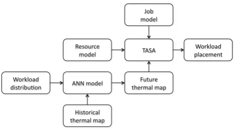
This section introduces the concept of the framework for thermal-aware workload scheduling as shown in Fig.1.

A thermal map is the temperature field in the data center space. A data center monitoring system, for example, either a temperature sensor-based monitoring service [12,16] or by using compute fluid dynamics software [10, 11], can generate a thermal map for a data center.

presents compute resource physical layout and its compute power characteristics.

With a data center model and historical thermal map, AI techniques like ANN can predicate future thermal maps for a data center.

Given a data center model (resource model and job model) and future thermal maps, a thermal-aware task scheduling algorithm (TASA) can place workloads on the proper compute nodes with the objective to reduce maxi-mum node temperature and task response time.

The workload placement can also predict future thermal maps and then give advice to future cooling system oper-ations. Cooling system operations can change future ther-mal maps.

6 ANN-based temperature prediction for a data center

This section discusses how we use an ANN to predict compute resource temperatures in a data center. We use ANN because we want our solution to be adaptable and suitable for real-time scheduling. With an ANN, our solution is adaptable because we can use real-time training, combined with our initial offline training phase, to improve the prediction performance over time. Our experimental results show that our trained ANN can produce good pre-dictions in a very small amount of time.

6.1 Problem formalization

At a high level, we would like a functionfthat can predict a valuePfor all given inputsI:

P¼fðIÞ ð13Þ

At a more detailed level, we can say we are attempting to predict a thermal map TempMap(t?Dt) for a given workload distribution W(t) and current thermal map TempMap(t). Then I= \W(t),TempMap(t)[in our case. Therefore, to predict nodep’s temperature, we

formalize the problem as follows:

nodep:TempðtþM_{tÞ ¼fðWðtÞ;TempMapðtÞÞ ð14Þ}

With the formal definition in Sect. 3, we have, TempMapðtÞ ¼ðnodei:\x;y;z[;nodei:TempðtÞÞnodei

2Node;1iI:g ð15Þ WðtÞ ¼jobj;nodelistjjobj2Job;jobj:tarrive

t;nodelistjNode;1jJ:g ð16Þ wherenodelistj is the node set that executesjobj.

6.2 Thermal impact matrix

The complexity of an ANN is based on the number of neurons contained in each layer of the network. The complexity has a direct effect on the ANN’s training and execution time. Since we want to use our ANN model in real-time scenarios, we want to make our ANN as simple, as possible while reducing its complexity. From our pre-vious discussion, we can see that using the complete thermal map in a data center produces a large input vector. We noticed that a node’s temperature is only affected significantly by two factors: the workload executed on it and the neighbor nodes’ temperatures. To help reduce the size of our input vector and the complexity of the ANN, we introduce aThermal Impact Matrixto reflect on the above two factors instead of using the data center’s complete thermal map:

A¼ ½ai;j ð17Þ

ai;j¼

1 if i¼j

nodej:TempðtÞnodei:TempðtÞ

Eðnodei;nodejÞ if i6¼j (

ð18Þ

whereIrepresents the number of nodes in the data center and ai,j present’s nodei’s spacial impact on nodej,

Eðnodei;nodejÞ is the Euler distance between nodei and

nodej, and 0i;jI. The Euler distance captures the

distance and space relationship between two nodes, for example, which nodes are placed lower or higher. Natu-rally, for a given node, the nodes directly below it will have a high impact, while nodes above it will not have as sig-nificant of an impact. Hence, we eliminate the impact between nodes that are far away from each other by ignoring them if they are below a certain threshold and we can setai,j=0. Therefore, most elements of Aiare 0 in a

large data center.

Now, to predict nodep’s temperature, the problem of

Eq. 14can be reduced as follows:

nodep:TempðtþM_{tÞ ¼fðnodep:TempðtÞ;Ap;joblistiÞ}

ð19Þ

wherejoblisti is the job set that executed onnodepduring

the time period ofM_{t;Ap¼ ½ap;1;ap;2;. . .;ap;j;. . .;ap;I}t_{. As}

most elements ofApare 0, the input vector for our ANN

model is thus much reduced.

6.3 Implementation

Several tools for ANN development are readily available, but we chose to go with the fast artificial neural network (FANN) library [30]. FANN provided us with several different ANN configurations, such as various activation functions and fully and partially connected ANNs.

For our experiments, we used both fully and partially connected multi-layered perceptron networks. For both types, we used three layers, an input, hidden, and an output layer. It is possible to have more layers, but this has shown to be often unnecessary [31].

First, we discuss our input layer. As we discussed in the previous section, for a given node nodep, our inputs are

nodep.Temp(t), the node’s partial impact matrix,Ap, and the

node’s job listjoblistp. Since most elements inApare 0, we

can prune these values from our input vector, resulting in the partial matrixAp. So, the size of our input vector is

N¼nodep:TempðtÞ þ jApj þ jjoblistpj ð20Þ

In our experience with data fromCCR, |Ap|&I/10,Iis the

total number of compute nodes in CCR.

Between the input and output layers, there exist a number of hidden layers, each consisting of any number of hidden neurons. There are several rules of thumb available to determine the number of hidden neurons for a given type of problem. The number of hidden neurons is often based on the number of input neurons. For our experiments, we choseN/2 hidden neurons.

For fully connected ANNs, the inputs for each neuron in the hidden layer is the output for each node in the input layer. Thus, in our experiment, each of the N/2 hidden neuron hadNinputs.

Each neuron applies a weightwito each of theNiinputs.

The weighted inputs are passed into the neurons activation function,a_function.

yi¼a function X N

i¼0 wiNi

!

ð21Þ

Ifyireaches a threshold, the neuron ‘‘fires’’, sending a

non-zero output to the neurons in the next layer. The most popular activation functions are the sigmoid activation functions. The sigmoid activation function only accepts values from [0, 1], so we scaled each of our inputs to fall with in this range.

With partially connected ANNs, each hidden neuron does not always accept N inputs. As many connections turn out to be irrelevant to the network, they get pruned off, thus reducing the complexity of the network. For our

experiments, we tested connectivity rates of 60, 70, 80, and 90%.

6.4 Experiment results and discussion

In this section, we will discuss the performance of our ANN.

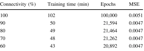
Several metrics are discussed, such as prediction accu-racy, training time, and execution time. We tested these metrics for several different ANN configurations. In the experiments, we use the temperature data collected from CCR as input, which was discussed in Sect. 8. For our experiments we set a MSE to 0.0047 and maximum num-ber of epochs to 100,000. The performance of our ANN implementation is shown in Table 1.

While connectivity is the percentage of connections between the input layer and the hidden layer, 100% is a fully connected ANN. Training time is how long it took for each network’s MSE to converge to our desired MSE of 0.0047. Epochs are the number of iterations on which the ANN had to train to reach the desired MSE. The MSE shows whether the network was able to converge to the desired MSE of 0.0047.

The partially connected networks outperformed the fully connected network, which was not able to converge to the desired MSE over 100,000 epochs. Each of the partially connected networks was able to predict a test job’s tem-perature profile in less than 1 s, making it suitable for our real-time scenario after training.

To test our accuracy, we compared the ANN’s predicted values to the real values obtained from the CCR data center. We tested these values using the 70% connectivity network. We depict prediction accuracy in Table2 and Fig.2. In Fig. 2, various compute nodes mean the index of compute nodes in the CCR cluster.

Table 1 Performance of ANN implementation

Connectivity (%) Training time (min) Epochs MSE

100 102 100,000 0.0051

90 50 21,594 0.0047

80 49 21,464 0.0047

70 48 21,262 0.0047

60 43 20,892 0.0047

Table 2 Predication accuracy of ANN model

Percentage of predictions Error (%)

42 ±1.5

65 ±2.5

7 Thermal-aware scheduling algorithm

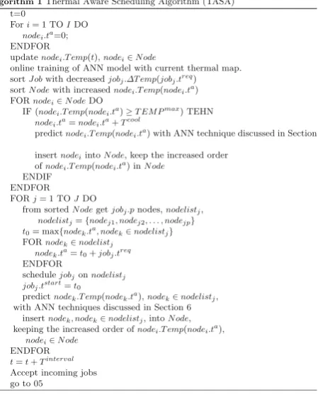
This section discusses our TASA. As shown in Fig.3, with periodically updated data center information, the TASA executes periodically to accept incoming jobs and schedule them to compute nodes of multiple racks.

A job’s task-temperature profile defines how ‘‘hot’’ a job is over time. The compute node’s temperature of its next available time,nodei.tacan be predicted by AI techniques

discussed in Sect.6. The key idea of TASA is to schedule ‘‘hot’’ jobs on ‘‘cold’’ compute nodes and tries to reduce the temperature increase of compute nodes. Algorithm 1 shows the details of TASA.

Algorithm 1 Thermal Aware Scheduling Algorithm (TASA)

Algorithm 1 presents the TASA. Lines 1–4 initialize variables. Line 1 sets the initial scheduling time stamp to 0. Lines 2–4 set compute nodes available time to 0, which means all nodes are available from the beginning.

Lines 5–29 of Algorithm 1 schedule jobs periodically with an interval of Tinterval. Lines 5 and 6 update current temperatures of all nodes from temperature sensors. Then line 7 sorts all jobs with decreased jobj:DTempðjobj:treq_Þ: jobs are sorted from ‘‘hottest’’ to ‘‘coolest’’. Line 8 sorts all nodes with increasing node temperature at the next avail-able time, nodei:Tempðnodei:taÞ: nodes are sorted from ‘‘coolest’’ to ‘‘hottest’’ when nodes are available.

Lines 9–14 cool down the over-heated compute nodes. If a node’s temperature is higher than a pre-defined temper-ature TEMPmax, then the node is cooled for a period of Tcool. During the period ofTcool, there is no job scheduled on this node. This node is then inserted into the sorted node list, which keeps the increased node temperature at next available time.

Lines 16–26 allocate jobs to all available compute nodes. Related research [21] indicated that, based on the Fig. 2 ANNs simulation result

standard model for the microprocessor thermal behavior, for any two tasks, scheduling the ‘‘hotter’’ job before the ‘‘cooler’’ one results in a lower final temperature. There-fore, Line 16 gets a job from the sorted job list, which is the ‘‘hottest’’ job, and line 17 allocates the job with a number of required nodes, which are the ‘‘coolest’’. Lines 18–20 find the earliest starting time on these nodes,nodelistj, for

jobj. After that, line 24 predicts the temperatures of next

available time for these nodes,nodelistj. Then these nodes

are inserted into the sorted node list, Node, keeping the increased node temperatures at next available time.

Algorithm 1 waits for a period ofTinterval and accepts incoming jobs. It then proceeds to the next scheduling round.

8 Simulation and performance evaluation

8.1 Simulation environment

We simulate a real data center environment based on the Center for Computational Research (CCR) of State Uni-versity of New York at Buffalo. All jobs submitted to CCR are logged during a 30-day period, from 20 Feb 2009 to 22 Mar 2009. CCR’s resources and job logs are used as input for our simulation of the TASA with backfilling.

CCR’s computing facilities include a Dell x86 64 Linux Cluster consisting of 1056 Dell PowerEdge SC1425 nodes, each of which has two Irwindale processors (2MB of L2 cache, either 3.0 GHz or 3.2 GHz) and varying amounts of main memory. The peak performance of this cluster is over 13 TFlop/s.

The CCR cluster has a single job queue for incoming jobs. All jobs are scheduled with a first come first serve (FCFS) policy, which means incoming jobs are allocated to the first available resources. There were 22,385 jobs sub-mitted to CCR during the period from 20 Feb 2009 to 22 Mar 2009.

In the following section, we simulate the TASA based on the job-temperature profile, job information, thermal maps, and resource information obtained in CCR log files. We evaluate the TASA by comparing it with the original job execution information logged in the CCR, which is scheduled by FCFS. In the simulation of TASA, we set the maximum temperature threshold (redline) to 125:5F. 8.2 Experiment results and discussion

8.2.1 Data center temperature

First, we consider the maximum temperature in a data center as it correlates with the cooling system operating

level. We userTempmax_{to show the maximum}

tempera-ture reduced by TASA. rTempmax_¼Tempmax

fcfs Temp

max

tasa ð22Þ

where Tempfcfsmax is the maximum temperature in a data

center where FCFS is employed, and Temptasamax is the

maximum temperature in a data center where TASA is employed.

In the simulation, we got rTempmax_¼6:67F.

There-fore, TASA reduces 6:67F of the average maximum temperatures of the 30-day period in CCR.

It is reported that every 1F reduced in a data center, 2% of the energy for the cooling system can be saved [4,5]. Therefore, TASA can save up to 13.34% power supply of CCR’s cooling system, which is up to 6.67% of CCR’s total power. It is estimated that CCR’s total power con-sumption is around 80,000 kW. Thus, the TASA can save around 5,330 kW power consumption.

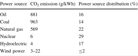
Table3 shows the environmental effect of power con-sumption. The left column shows the power sources; the second column shows the CO2emission of different power sources [32]. The right column shows the power source distribution in New York state [33]. Based on Table3, we can coarsely estimate that CCR costs around 33,000 kg CO2emission every hour, and TASA can reduce 2,130 kg CO2 emission per hour. The emission produced over a year’s timespan equates to about 37 thousand midsize cars [34]. We also consider the average temperatures in a data center, which relates the system reliability. Compared with FCFS, the average temperature reduced by TASA is 17:9F:

8.2.2 Job response time

We have reduced power consumption and have increased the system reliability, both by decreasing the data center temperatures. However, we must consider that there may be trade offs to be considered, such as an increased response time.

Table 3 Environment effect of power consumption

Power source CO2emission (g/kWh) Power source distribution (%)

Oil 881 16

Coal 963 14

Natural gas 569 22

Nuclear 6 29

Hydroelectric 4 17

The response time of a job jobj.tres is defined as job

execution time (jobj.treq) plus job queueing time

ðjobj:tstartjobj:tarriveÞ, as shown below:

jobj:tres¼jobj:treqþjobj:tstartjobj:tarrive ð23Þ

To evaluate the algorithm from the user’s point of view, the job response time indicates the time it takes for results to return to the users.

As TASA intends to delay the scheduling of jobs to compute nodes that are assumed to be too hot, it may increase the job response time. Figure4 shows the

response time of the FCFS, and Fig. 5shows the response time of TASA.

In the simulation, we calculate the overall job response time overhead as follows:

overhead¼ X

1jJ

jobj:t_tasares jobj:tres_fcfs jobj:tres

fcfs

ð24Þ

In the simulation, we obained an overhead of 15.2%, which means that we reduced the maximum temperature by 6:67F and the average temperature by 17:9F in CCR’s data center by paying cost of increasing the job response time by 15.2%.

8.2.3 Data center utilization

Another important performance metric is the data center space utilization. Data center space utilization indicates how much percent of total resources are busy at any spe-cific point in time. The system utilization, which is affected by the policy workload placement, has an important impact on the cooling cost. For certain system utilization, different workload placement policies, for example, in our context TASA and FCFS have different cooling costs, which has been discussed above.

Since our simulation uses the same workload as input for TASA and FCFS, the simulations for TASA and FCFS have the same overall system utilization. However, in different time periods, TASA and FCFS have different system utilization, as shown in Fig.6. Here, the blue line shows the data center space utilization scheduled by the FCFS, and the red line shows the data center space utili-zation by the TASA. We can see that the data center space utilization under the FCFS and the TASA are in alternative trends: during certain periods, the data center space utili-zation under TASA is higher than that of FCFS; in the subsequent period, the data center space utilization under the FCFS is higher than that of the TASA. This can be explained as follows:

• When some jobs arrive at a data center, the TASA tries to distribute them to different compute resources to reduce a temperature increase. This means more resources are busy leading to a higher data center space utilization.

• As jobs may fill up compute resources in a data center, some resources reach the maximum temperature (125:5F), TASA delays the job submission and let resources cool down. However, FCFS does not consider the data center temperature and continues to schedule jobs to resources. This leads a higher data center space utilization.

Fig. 4 Job response time of FCFS

8.2.4 Compute performance versus Green metrics: a tradeoff

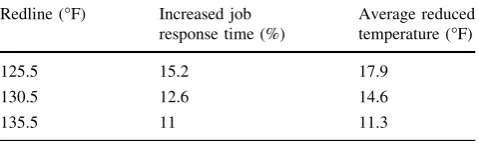
It is clear that we can reduce the compute nodes’ temper-atures in a data center by increasing the task response time. Obviously there is a tradeoff between them. Table4shows our simulation results of TASA by setting different redline values for a data center, hence, verifying a tradeoff between reduced average temperature and increased task response time.

9 Conclusion

Nowadays, energy-aware management of data centers is becoming more important in the context of Cloud and Green computing. Thermal-aware resource management of data centers can offer various benefits, like reducing cooling cost and increasing reliabilities of computing resources, thus promoting an environmental conscious computing paradigm. In this paper, we have developed an ANN-based temperature prediction implementation, which is lightweight and suitable for real-time scheduling sce-narios. This paper thereafter presents a method for data centers to reduce the temperatures in a data center, based on our ANN temperature predication. The algorithm is evaluated through a simulation based on real operational information from CCR’s data center. Test results and a performance discussion justify the design and implemen-tation.

Acknowledgments Work conducted by Lizhe Wang and Gregor von Laszewski is supported (in part) by NSF 0963571 and 2010 HP Annual Innovation Research Awards. Work conducted by Fang Huang is supported by the Fundamental Research Funds for the Central Universities (Grant No. ZYGX2009J073), the National Natural Science Foundation of China (Grant No. 41001221).

References

1. U.S. Environmental Protection Agency (2007) Report to Congress on Server and DataCenter Energy Efficiency. Technical Report, U.S. Environmental Protection Agency. Available at http:// www.energystar.gov/ia/partners/prod_development/downloads/ EPA_Datacenter_Report_Congress_Final1.pdf

2. The Green Grid (2007) The green grids opportunity: decreasing datacenter and other IT energy usage patterns. Technical report, the green grid association. Available at http://www. webhostingunleashed.com/whitepaper/decreasing-datacenter-energy-greengrid/

3. Sawyer R (2004) Calculating total power requirements for data centers. Technical report, American Power Conversion. Available athttp://dcmms.com/whitepapers/2.pdf

4. Best Practices for Energy Efficiency in Microsoft Data Center Operations, Fact Sheet (2008). http://download.microsoft.com/ download/a/7/b/a7b72ab1-ca17-4589-923a-83b0ff57be6d/Energy- Efficiency-Best-Practices-in-Microsoft-Data-Center-Operations-CeBIT.doc

5. Patterson MK (2008) The effect of data center temperature on energy efficiency. In: Proceedings of the 11th intersociety con-ference on thermal and thermomechanical phenomena in elec-tronic systems, pp 1167–1174, May 2008

6. Sharma RK, Bash CE, Patel CD, Friedrich RJ, Chase JS (2007) Smart power management for data centers. Technical report, HP Laboratories

7. Moore J, Chase J, Ranganathan P (2006) Weatherman: auto-mated, online, and predictive thermal mapping and management for data centers. In: The 3rd IEEE international conference on autonomic computing, June 2006

8. Hale PW (1986) Acceleration and time to fail. Qual Reliab Eng Int 2(4):259–262

9. Anderson D, Dykes J, Riedel E (2003) More than an interface— scsi vs. ata. In: Proceedings of the conference on file and storage technologies

10. Choi J, Kim Y, Sivasubramaniam A, Srebric J, Wang Q, Lee J (2008) A CFD-based tool for studying temperature in rack-mounted servers. IEEE Trans Comput 57(8):1129–1142 Fig. 6 Data center space utilization

Table 4 Compute performance versus Green metrics

Redline (F) Increased job response time (%)

Average reduced temperature (F)

125.5 15.2 17.9

130.5 12.6 14.6

11. Abdlmonem H, Patel CD (2007) Thermo-fluids provisioning of a high performance high density data center. Distrib Parallel Databases 21(2–3):227–238

12. Tang Q, Gupta SKS, Varsamopoulos G (2008) Energy-efficient thermal-aware task scheduling for homogeneous high-perfor-mance computing data centers: a cyber-physical approach. IEEE Trans Parallel Distrib Syst 19(11):1458–1472

13. Moore JD, Chase JS, Ranganathan P, Sharma RK (2005) Making scheduling ‘‘cool’’: temperature-aware workload placement in data centers. In: USENIX annual technical conference, General Track, pp 61–75

14. Mukherjee T, Tang Q, Ziesman C, Gupta SKS, Cayton P (2007) Software architecture for dynamic thermal management in data-centers. In: COMSWARE

15. Tang Q, Gupta SKS, Varsamopoulos G (2007) Thermal-aware task scheduling for data centers through minimizing heat recir-culation. In: CLUSTER, pp 129–138

16. Tang Q, Mukherjee T, Gupta SKS, Cayton P (2006) Sensor-based fast thermal evaluation model for energy efficient high-perfor-mance datacenters. In: Proceedings of the 4th international con-ference on intelligent sensing and information processing, Oct 2008, pp 203–208

17. Hoke E, Sun J, Strunk JD, Ganger GR, Faloutsos C (2006) InteMon: continuous mining of sensor data in large-scale self-infrastructures. Oper Syst Rev 40(3):38–44

18. Heath T, Centeno AP, George P, Ramos L, Jaluria Y (2006) Mercury and freon: temperature emulation and management for server systems. In: ASPLOS, pp 106–116

19. Ramos L, Bianchini R (2008) C-Oracle: predictive thermal management for data centers. In: HPCA, pp 111–122

20. Vanderster DC, Baniasadi A, Dimopoulos NJ (2007) Exploiting task temperature profiling in temperature-aware task scheduling for computational clusters. In: Asia-Pacific computer systems architecture conference, pp 175–185

21. Yang J, Zhou X, Chrobak M, Zhang Y, Jin L (2008) Dynamic thermal management through task scheduling. In: ISPASS, pp 191–201

22. Chrobak M, Du¨rr C, Hurand M, Robert J (2008) Algorithms for temperature-aware task scheduling in microprocessor systems. In: AAIM, pp 120–130

23. Wang L, von Laszewski G, Dayal J, He X, Younge AJ, Furlani TR (2009) Towards thermal aware workload scheduling in a data center. In: Proceedings of the 10th international symposium on pervasive systems, algorithms and networks (ISPAN2009), Kao-Hsiung, Taiwan, 14–16 Dec 2009

24. Wang L, von Laszewski G, Dayal J, He X, Younge AJ, Furlani TR (2009) Thermal aware workload scheduling with backfilling for green data centers. In: Proceedings of the 28th IEEE inter-national performance computing and communications confer-ence, Arizona, Dec 2009

25. Simon H (1994) Neural networks: a comprehensive foundation. Macmillan, New York

26. Ceravolo F, De Felice M, Pizzuti S (2009) Combining back-propagation and genetic algorithms to train neural networks for ambient temperature modeling in Italy. In: Applications of evo-lutionary computing, EvoWorkshops 2009, pp 123–131 27. Thomas B, Soleimani-Mohseni M (2007) Artificial neural

net-work models for indoor temperature prediction: investigations in two buildings. Neural Comput Appl 16(1):81–89

28. Smith BA, McClendon RW, Hoogenboom G (2005) An enhanced artificial neural network for air temperature prediction. In: International enformatika conference, pp 7–12

29. Jackowska-Strumillo L (2004) Ann based modelling and cor-rection in dynamic temperature measurements. In: 7th interna-tional conference artificial intelligence and soft computing, pp 1124–1129

30. Nissen S Fast artificial neural network library (FANN). Software libraries. Available athttp://http://leenissen.dk/fann/

31. Trenn S (2008) Multilayer perceptrons: approximation order and necessary number of hidden units. IEEE Trans Neural Netw 19(5):836–844

32. Carbon dioxide emissions from the generation of electric power in the United States (2009). Available athttp://www.eia.doe.gov/ cneaf/electricity/page/co2_report/co2report.htmlWebsite, Jun 2009 33. U.S. power grid visualization (2009). Available athttp://www.

eia.doe.gov/cneaf/electricity/page/co2_report/co2report.html 34. CO2 emission calculator (2007). Available at http://www.