RIT Scholar Works
Theses
Thesis/Dissertation Collections
2012
A MEMS viscosity sensor for conductive fluids
Luis Gan Chau
Follow this and additional works at:
http://scholarworks.rit.edu/theses
This Thesis is brought to you for free and open access by the Thesis/Dissertation Collections at RIT Scholar Works. It has been accepted for inclusion in Theses by an authorized administrator of RIT Scholar Works. For more information, please [email protected].
Recommended Citation
A MEMS VISCOSITY SENSOR FOR
CONDUCTIVE FLUIDS
by
Luis Alberto Gan Chau
A Thesis submitted in partial fulfillment of the requirements for the degree of
M
ASTER
OF
S
CIENCE
IN
ELECTRICAL ENGINEERING
Approved by:
Prof.
Thesis Advisor
– Dr. Lynn F. Fuller
Prof.
Thesis Advisor
– Dr. Ivan Puchades
Prof.
Thesis Advisor
– Dr. Sergey E. Lyshevski
Prof.
Department Head
– Dr. Sohail A. Dianat
Department of Electrical and Microelectronic Engineering
Kate Gleason College of Engineering
R
OCHESTER
I
NSTITUTE
OF
T
ECHNOLOGY
Rochester, New York
D
EDICATION
To my parents, sister, brothers and family, who in the distance have been supportive of
all my decisions:
"What this power is, I cannot say. All I know is that it exists...and it becomes available only
when you are in that state of mind in which you know exactly what you want...and are fully
determined not to quit until you get it."
A
CKNOWLEDGEMENTS
To my fellow colleagues, faculty, and mentors thanking you is the least I could do, but I
will always remember you for how much you have helped me change as a person and become a
better engineer.
To Dr. Lynn Fuller and Dr. Ivan Puchades who were present at all times helping me
accomplish this project. Without your guidance, I would have not learned the graduate aspect of
the research environment. Pushing me all the time to make sure I understand what I was doing
every step of this project. At the same time thinking in what needed to be done, and the
consequences of following the decisions made, and WHY that decision was taken with
background knowledge. That is the biggest one I will always remember, the special “WHY”.
To Dr. Sergey Lyshevski who helped me comprehend the different ways actual theorems
are solved, and why we use those theorems in different applications. Without that background I
would have not understood how and why it was occurring.
To Team GALT, Dan, Nick, you two have helped me see how to take the different paths
in life. Regardless of the path just make sure to take the easiest and shortest path rather than the
hardest and longest one. Understanding how to work as a team and provide insight regardless of
how much experience one has, it is always good to have different point of views.
“It is always the simple things that change our lives.”
A
BSTRACT
Outline
DEDICATION ... II
ACKNOWLEDGEMENTS ... III
ABSTRACT ... IV
LIST OF TABLES ... VII
LIST OF FIGURES ... IX
1.0
INTRODUCTION
... 1
1.1.0
QUICK OVERVIEW OF DEVICE (PROBLEM STATEMENT)
... 2
1.2.0
MICRO-ELECTRO MECHANICAL SYSTEMS (MEMS) & BIOMEDICAL-MEMS (BIO-MEMS)
... 3
1.3.0
VISCOSITY SENSORS
... 5
2.0
THERMALLY ACTUATED VISCOSITY SENSOR ... 8
2.1.0
ELECTRICAL COMPONENTS
... 8
2.1.1
Heater
... 8
2.1.2
The Wheatstone Bridge Circuit
... 9
2.2.0
PHYSICAL COMPONENTS
... 15
3.0
TESTING OF EXISTING VISCOSITY SENSOR WITH PACKAGING METHOD VERSION 1 ... 21
3.1.0
SCREENING EXPERIMENT
... 21
3.1.1
Calculating the frequency in Air
... 24
3.1.2
Calculating the frequency in a Fluid
... 25
3.1.3
Determining the L2T and Pulse Time for good output
... 26
3.1.4
Determining Heater voltage and gain
... 30
3.2.0
STEPS FOR PACKAGING DIE TO PCB
... 30
3.3.0
TESTING OF SENSOR WITH VERSION 1
... 32
3.3.1
Test Setup
... 33
3.3.2
Test Results
... 34
3.3.3
Observations from testing devices in Air
... 35
3.3.4
Nail Polish Selection (Nail Aid or Sally Hansen)
... 36
3.3.5
Observations from testing devices in a conductive fluid
... 40
3.4.0
PROBLEMS TO CURRENT SENSOR WITH PACKAGING VERSION 1
... 44
3.5.0
PROPOSED SOLUTIONS TO CURRENT SENSOR
... 45
4.0 TESTING OF SENSORS IN OIL BEFORE ADDING PROTECTIVE LAYER AND AFTER ADDING
PROTECTIVE LAYER ... 50
4.1.0
OUTPUT SIGNAL
... 52
4.2.0
SENSOR OILS TEST BEFORE PARYLENE C PROTECTIVE LAYER
... 53
4.3.0
PARYLENE COATER TOOL (VERSION 2)
... 60
4.3.2
Determining thickness of Parylene C from 1
sttrial
... 66
4.3.3
Measuring film thickness using Tencor P2
... 67
4.3.4
Determining Mass of Dimer required for specific thicknesses
... 68
4.3.5
Strength Test of Parylene C Thin Film
... 69
4.3.6
Testing protective layer on a different sensor in a conductive fluid
... 70
4.3.7
Theoretical Calculations of adding a layer of Parylene C
... 73
4.4.0
TESTING SENSORS WITH PARYLENE C IN AIR
... 77
4.5.0
COMPARISON BETWEEN SENSORS BEFORE AND AFTER PARYLENE C LAYER
... 78
5.0 PROTECTIVE LAYER VERSION 2 TESTS IN CONDUCTIVE FLUIDS ... 85
5.1.0
SENSORS WITH PARYLENE C IN 24HRS TEST
... 85
5.1.1
Procedure test setups
... 85
5.1.2
Sensor Test Results in conductive fluid
... 88
5.1.3
Problems while testing in conductive fluid
... 94
5.1.4
Summary of 24-hour test
... 95
5.2.0
SENSORS WITH PARYLENE C IN CONDUCTIVE FLUIDS AT DIFFERENT VISCOSITIES
... 96
5.2.1
Glycerol
... 96
5.2.2
Glycerol Water Mixture
... 97
5.2.3
Determining viscosity values of glycerol water mixtures at 25°C
... 97
5.2.4
Making the conductive fluid for different viscosity values
... 99
5.2.5
Glycerol Water Mixture tests
... 100
6.0
REPEATABILITY & ACCURACY
... 104
6.1.0
TEST SETUP FOR REPEATABILITY AND ACCURACY
... 104
6.2.0
RESULTS FOR REPEATABILITY
... 105
6.3.0
RESULTS FOR ACCURACY
... 106
6.4.0
CONCLUSION FOR REPEATABILITY & ACCURACY
... 107
7.0
CONCLUSIONS
... 108
7.1.0
FUTURE WORK
... 108
8.0
APPENDIX
... 110
List of Tables
TABLE 3.1-EXAMPLE OF MEASUREMENTS OBTAINED FROM A SINGLE DIE FROM WAFER 3 ... 22
TABLE 3.2-DEVICES 1 THROUGH 10 WITH CHARACTERISTICS FROM WAFER 3 ... 23
TABLE 3.3-MEASUREMENTS TO CALCULATE THE FREQUENCY IN AIR OF A DEVICE FROM WAFER 3 ... 24
TABLE 3.4-CALCULATED FREQUENCIES IN AIR AT A GIVEN THICKNESS AND LENGTH SIZE,A ... 24
TABLE 3.5-NEW COLUMN ADDED TO TABLE 1 WITH CALCULATED FREQUENCY IN AIR VALUE ... 25
TABLE 3.6-PARAMETERS TO CALCULATE THE FREQUENCY OF THE SENSOR IN A FLUID ... 25
TABLE 3.7–LENGTH TO CRITICAL THICKNESS RATIO COLUMN ... 26
TABLE 3.8-INFORMATION ON L2T RATIOS FOR ALL THE DIFFERENT DEVICES ... 27
TABLE 3.9-TIME REQUIRED FOR HEAT PULSE TO ACTIVATE SENSOR ... 28
TABLE 3.10-TIME REQUIRED FOR SENSOR TO ACTIVATE MEMBRANE ACCORDING TO THEIR CHARACTERISTICS ... 29
TABLE 3.11-SENSOR CHARACTERISTICS FOR DEVICE I3 ... 35
TABLE 3.12-TEST RESULTS FOR SENSOR 5B ... 44
TABLE 3.13-PHYSICAL PROPERTIES FROM DIFFERENT SOURCES REGARDING MATERIALS FOR ENCAPSULATION ... 47
TABLE 4.1-VISCOSITY AND DENSITY VALUES FOR STANDARIZED OILS AT ROOM TEMPERATURE ... 50
TABLE 4.2-SENSORS CHARACTERISTICS ... 50
TABLE 4.3-SENSORS CHARACTERISTICS WITH THEIR CORRESPONDING VALUES ... 53
TABLE 4.4-POWER LAW FIT OF NORMALIZED FREQUENCY AVERAGES ... 56
TABLE 4.5-PREDICTED EXCEL EQUATIONS FOR AMPLITUDE RESULTS ... 58
TABLE 4.6-QUALITY FACTOR R2THEORETICAL CALCULATIONS ... 59
TABLE 4.7-L2TRATIOS CORRESPONDING TO THE HEATER SIZE ... 60
TABLE 4.8-TESTING MEASUREMENTS FOR THICKNESS OF THIN FILM ... 67
TABLE 4.9-MASS REQUIRED TO PRODUCE DESIRED THICKNESS OF THIN FILM ... 69
TABLE 4.10-TEST RESULTS OF SENSORS WITH PARYLENE C IN OILS AND DEIONIZED WATER ... 72
TABLE 4.11-DENSITY AND YOUNG'S MODULUS OF SILICON AND PARYLENE C ... 75
TABLE 4.12-VOLUME CALCULATIONS FOR RELATION WITH MASS ... 76
TABLE 4.13-MASS CALCULATIONS USING DATA FROM PREVIOUS TABLE ... 76
TABLE 4.14-SPRING CONSTANT CALCULATIONS ... 76
TABLE 4.15-MASS PERCENT CHANGE ACCORDING TO THEIR LENGTHS AND THICKNESSES ... 76
TABLE 4.16-SPRING CONSTANT PERCENT CHANGE WITH RESPECT TO THICKNESS OF PARYLENE C ... 76
TABLE 4.17-INFORMATION ON SENSORS WITH PARYLENE C ... 77
TABLE 4.18-INFORMATION ON OUTPUT OF SENSORS ... 77
TABLE 4.19-INFORMATION ON 3 SENSORS WITH PROTECTIVE LAYER VERSION 2 ... 79
TABLE 4.20-NORMALIZED FREQUENCY POWER LAW FIT APPLIED TO DATA IN OILS TO DEVICES WITH NO PARYLENE C LAYER ... 80
TABLE 4.21-NORMALIZED FREQUENCY POWER LAW FIT APPLIED TO DATA IN OILS TO DEVICES WITH PARYLENE C LAYER ... 81
TABLE 4.22-VRMS POWER LAW FIT TO DATA ON SENSORS WITH NO PARYLENE C ... 82
TABLE 4.23-VRMS POWER LAW FIT TO DATA ON SENSORS WITH PARYLENE C ... 82
TABLE 4.24-NORMALIZED Q POWER LAW FIT TO DATA ON SENSORS WITH NO PARYLENE C ... 83
TABLE 4.25-NORMALIZED Q POWER LAW FIT TO DATA ON SENSORS WITH PARYLENE C ... 83
TABLE 4.26-FREQUENCY % CHANGE WITH INCREASING VISCOSITY FOR SENSORS WITH AND WITHOUT PARYLENE C 84
TABLE 4.27-QUALITY FACTOR % CHANGE WITH INCREASING VISCOSITY FOR SENSORS WITH AND WITHOUT PARYLENE C ... 84
TABLE 5.2-INFORMATION ON TESTING 3 SENSORS IN DEIONIZED WATER ... 91
TABLE 5.3- SUMMARY OF DIFFERENT EQUATIONS TO DETERMINE VISCOSITY OF GLYCEROL WATER MIXTURES ... 97
TABLE 5.4-INFORMATION TO CALCULATE VISCOSITY USING DIFFERENT REFERENCES [4243] ... 98
TABLE 5.5-DETERMINING GLYCERIN % WT FOR MIXTURES ... 100
TABLE 5.6-SENSORS CHARACTERISTICS FOR CONDUCTIVE FLUIDS WITH VARYING VISCOSITY TEST ... 100
TABLE 5.7-POWER LAW FIT TO THE RESULTS FROM DEVICE L1 ... 103
TABLE 1A-RESULTS FROM SCREENING EXPERIMENT ... 110
TABLE 2A-VISCOSITY OF AQUEOUS GLYCERIN SOLUTIONS IN (CP) OR (mPA*S)[4846] ... 112
TABLE 3A-CALCULATED VALUES OF VISCOSITY FOR DIFFERENT GLYCERIN PERCENT WEIGHT AT 20°C ... 113
TABLE 4A-CALCULATED VALUES COMPARED WITH DORSEY REFERENCE AS TEMPERATURE IS INCREASED THE VISCOSITY DECREASES ... 114
List of Figures
FIGURE 1.1–THERMALLY ACTUATED VISCOSITY SENSOR MEMS SENSOR TOP VIEW [1] ...2
FIGURE 1.2-NEOSENSE WAFER WITH NUMEROUS MEMS DEVICES [2] ...3
FIGURE 1.3-EMERGING MEMS MARKET WORLDWIDE [5] ...4
FIGURE 1.4–MEMSPRESSURE SENSOR FOR AUTOMOTIVE INDUSTRY (LEFT)[7]BOSCH MEMSDIGITAL PRESSURE SENSOR (RIGHT)[8] ...4
FIGURE 1.5-MEMSGLUCOSE MONITORING SYSTEM [10] ...6
FIGURE 1.6-RESULTS FROM VISCOSITY SENSOR OF FREQUENCY AND QFACTOR IN DIFFERENT SUGAR SOLUTIONS[11] ...7
FIGURE 2.1-HEATER CIRCUIT SCHEMATIC ...8
FIGURE 2.2-WHEATSTONE BRIDGE DESIGN [20],[21] ...9
FIGURE 2.3-WHEATSTONE BRIDGE DESIGN USED FOR ANALYSIS ...10
FIGURE 2.4-BEST LOCATION FOR THE RESISTORS ON A THEORETICAL MEMBRANE ...12
FIGURE 2.5-HEATER AND POWER MOSFET SCHEMATICS ...13
FIGURE 2.6-INSTRUMENTATION AMPLIFIER (INA-101HP) ...14
FIGURE 2.7-INSTRUMENTATION AMPLIFIER CIRCUITRY (INA-101HP)[22] ...14
FIGURE 2.8-EXAMPLE OF OUTPUT FROM A SENSOR IN GLYCEROL-WATER MIXTURE ...15
FIGURE 2.9-DIAPHRAGM ON XYZ COORDINATE TO DEFINE DIRECTION OF DEFLECTION [23] ...16
FIGURE 2.10-DIAPHRAGM ON XY COORDINATE ...16
FIGURE 2.11-TEMPERATURE INCREASE OF A MEMBRANE IN AIR AND OIL FOR PULSED HEATING [1] ...17
FIGURE 2.12-FFT FOR DEVICE 1P, USED TO DETERMINE Q[1] ...19
FIGURE 2.13-NORMALIZED FREQUENCY AND Q FACTOR VERSUS KINEMATIC VISCOSITY AND TEMPERATURE [1] ...20
FIGURE 3.1-AN OVERVIEW OF HOW THE DEVICES WERE TESTED ...21
FIGURE 3.2-ELECTRICAL SCHEMATIC OF THE WHEATSTONE BRIDGE ...22
FIGURE 3.3-GRAPH SHOWING PULSE FROM SIGNAL GENERATOR ...29
FIGURE 3.4- BEFORE (RIGHT) AND AFTER (LEFT) CLEANING IMPURITIES FROM PCBS ...31
FIGURE 3.5-PCB PACKAGED AND READY FOR TESTING ...32
FIGURE 3.6-PCB LAYOUT WITH DRILLED HOLES AND TOP HOLE FOR DIAPHRAGM PLACEMENT ...32
FIGURE 3.7-PCB LAYOUT WITH SENSOR AND WIRE BONDS ...32
FIGURE 3.8-PCB LAYOUT WITH SENSOR AND EPOXIED FOR PROTECTION ...32
FIGURE 3.9-BLOCK DIAGRAM OF VISCOSITY DETECTION ...33
FIGURE 3.10-AVIEW OF THE OSCILLOSCOPE WITH THE 2 REQUIRED SIGNALS ...34
FIGURE 3.11-NAIL POLISH (LEFT) AND 5 MINUTE EPOXY (RIGHT) ...34
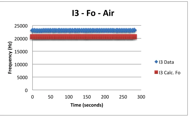
FIGURE 3.12-FREQUENCY RESPONSE OF SENSOR I3 IN AIR ...36
FIGURE 3.13-QUALITY FACTOR (LEFT) AND AMPLITUDE (RIGHT) ...36
FIGURE 3.14-APPLICATION OF NAIL POLISH ON TO THE PCB BOARD AND NEAR THE SENSOR ...37
FIGURE 3.15-ELECTRICAL SCHEMATIC OF TESTING A PCB WITH NAIL POLISH INSIDE A BEAKER WITH DEIONIZED WATER ...37
FIGURE 3.16-NAIL POLISH CONTAINERS SALLY HANSEN (LEFT),NAIL AID (RIGHT) ...38
FIGURE 3.17-NAIL POLISH SH CLEAR AND THIN LAYER (LEFT) AND NA BUBBLES WITH THICKER LAYER (RIGHT) ...38
FIGURE 3.18-NAIL POLISH SH CLEAR (LEFT) AND EPOXY BUBBLY (RIGHT) ...39
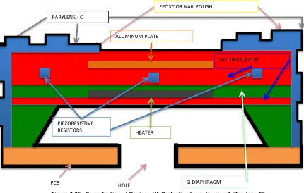
FIGURE 3.19-CROSS SECTION OF SENSOR WITH PROTECTIVE LAYER VERSION 1(EPOXY OR NAIL POLISH) ...40
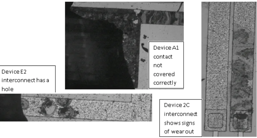
FIGURE 3.20-OVERVIEW OF SOME OF THE VISIBLE PROBLEMS USING A MICROSCOPE OCCURRING TO THE SENSORS ...41
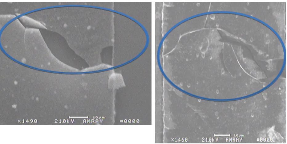
FIGURE 3.21-SEMS @1490X OF BROKEN INTERCONNECTS ...42
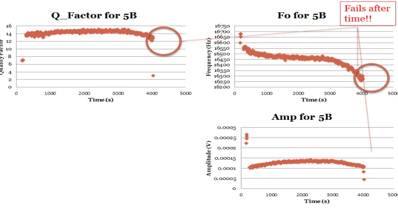
FIGURE 3.22-RESULTS FROM DEVICE 5B WHILE TESTING UNDERWATER ...43
FIGURE 3.23-SENSOR 5B TESTING IN DEIONIZED WATER ...43
FIGURE 3.25-CROSS SECTION OF DEVICE WITH PROTECTIVE LAYER VERSION 2(PARYLENE C) ...48
FIGURE 3.26-PROTECTIVE LAYER VERSION 2-TOP VIEW OF PCB+ DIE +PARYLENE COATING +EPOXY ...48
FIGURE 4.1-OILS S3,N10,N35,5W30 IN THEIR RESPECTIVE VIALS ...51
FIGURE 4.2-SENSOR PLACED INSIDE A VIAL READY FOR TAKING MEASUREMENTS ...51
FIGURE 4.3-SENSOR OUTPUT IN AIR ...52
FIGURE 4.4-THEORETICAL CALCULATIONS OF NORMALIZED FREQUENCY FOR DIFFERENT VISCOSITY VALUES ...54
FIGURE 4.5-NORMALIZED FREQUENCY VARIATION IN DIFFERENT OIL SAMPLES ...55
FIGURE 4.6-AMPLITUDE VARIATION WITH DIFFERENT SENSOR CAHRACTERISTICS IN DIFFERENT OILS SAMPLES ...57
FIGURE 4.7-SENSOR PLACED INSIDE THE VIAL IN THE WRONG POSITION ...58
FIGURE 4.8-NORMALIZED QUALITY FACTOR WITH SENSOR VARIATION CHARACTERISTICS ...59
FIGURE 4.9-L2T RATIO VS FREQUENCY ...60
FIGURE 4.10-PARYLENE COATER TOOL MADE IN HOUSE BY DR.ALAN RAISANEN AND HIS TEAM AT RIT ...61
FIGURE 4.11-PARYLENE C DIMER (SPECIALTY COATING SYSTEMS) ...62
FIGURE 4.12- CHEMICAL PROCESS INSIDE PARYLENE COATER TOOL WITH PARYLENE C ...63
FIGURE 4.13-MICRO 90, REAGENT USED TO PREVENT THIN FILM FROM STICKING TO ANY SURFACE ...63
FIGURE 4.14-EVAPORATION CHAMBER COVERED WITH ALUMINUM FOIL (LOCATION FOR BOAT WITH PARYLENE C DIMER) ...64
FIGURE 4.15-BOATS HAND MADE FROM ALUMINUM FOIL TO HOLD PARYLENE C DIMER PELLETS ...64
FIGURE 4.16-SMALLER BOAT USED TO WEIGHT PARYLENE C INSIDE SCALE ...65
FIGURE 4.17-A-174SILANE, ADHESION PROMOTER (LEFT), SENSOR INSIDE BEAKER WITH A-174(RIGHT) ...65
FIGURE 4.18-SENSORS INSIDE THE CHAMBER NEXT TO A GLASS SLIDE ...66
FIGURE 4.19-KLATENCOR P2PROFILOMETER ...67
FIGURE 4.20-GLASS SLIDE FOR THICKNESS MEASUREMENTS OF PARYLENE C RUNS ...68
FIGURE 4.21-ANOTHER GLASS SLIDE FOR THICKNESS MEASUREMENTS OF PARYLENE C ...68
FIGURE 4.22-DETERMINING MASS REQUIRED OF PARYLENE C FOR DESIRED THIN FILM THICKNESS ...69
FIGURE 4.23-VISIBLE CRACK CAUSES CLEANING PROBLEMS ...70
FIGURE 4.24-RESISTOR DESIGN FROM NICHOLAS LIOTTA ...71
FIGURE 4.25-THREE DUMMY SENSORS TO TEST THIN PROTECTIVE FILM ...71
FIGURE 4.26-ELECTRICAL SCHEMATICS FOR TESTING HEATER LIKE DEVICES IN DEIONIZED WATER ...72
FIGURE 4.27- SENSOR 15 WITH PARYLENE C COATING TESTING IN DEIONIZED WATER ...73
FIGURE 4.28-SENSOR VIEW AFTER ADDING A THIN LAYER OF PARYLENE C ...74
FIGURE 4.29-NORMALIZED FREQUENCY RESPONSE OF SENSORS BEFORE AND AFTER PARYLENE C ...79
FIGURE 4.30-NORMALIZED VRMS OF SENSORS BEFORE / AFTER PARYLENE C ...81
FIGURE 4.31-NORMALIZED Q FACTOR OF SENSORS BEFORE / AFTER PARYLENE C ...82
FIGURE 5.1-SENSOR I3 INSIDE DEIONIZED WATER FOR LONG TERM TESTING ...87
FIGURE 5.2-SENSOR HOLDER PIECE THAT FITS PERFECTLY ON TOP OF A VIAL ...87
FIGURE 5.3-SENSOR G1 PLACED INSIDE THE PIECE HOLDER ...88
FIGURE 5.4-SENSOR IN DEIONIZED WATER WITHOUT PIECE HOLDER ...88
FIGURE 5.5-CROSS SECTION OF DEVICE WITH VERSION 2 IN CONDUCTIVE FLUID ...89
FIGURE 5.6-SIGNAL FOR THE FIRST 10 MINUTES (LEFT) AFTER THE SIGNAL STARTS TO FADE (RIGHT) ...90
FIGURE 5.7-LONG TERM TESTING RESULTS FOR NORMALIZED FREQUENCY FOR 3 DIFFERENT SENSORS ...92
FIGURE 5.8-LONG TERM TESTING RESULTS FOR NORMALIZED AMPLITUDE FOR 3 DIFFERENT SENSORS ...92
FIGURE 5.9-LONG TERM TESTING RESULTS FOR NORMALIZED QFACTOR FOR 3 DIFFERENT SENSORS ...93
FIGURE 5.10-CONDUCTIVE FLUID LONG TERM TEST ...93
FIGURE 5.11-DATA CABLE WITH EPOXY AROUND THE SOLDERED PINS ...94
FIGURE 5.12-NEW SETUP WITH LONGER "INSULATED" CABLE, TOGETHER WITH THE PIECE HOLDER AND AN EMPTY VIAL ...94
FIGURE 5.15-NORMALIZED AMPLITUDE RESPONSE IN GLYCEROL WATER MIXTURES ...102
FIGURE 5.16-NORMALIZED QUALITY FACTOR RESPONSE IN GLYCEROL WATER MIXTURES ...102
FIGURE 6.1-NORMALIZED FREQUENCY RESULTS FOR REPEATABILITY OF SENSOR J5 AT 1HZ AND 20HZ ...105
FIGURE 6.2-REPEATABILITY AT 84.67%GLYCEROL WATER MIXTURE AT A FREQUENCY OF 1HZ ...106
FIGURE 6.3-ACCURACY TEST AT HIGH AND LOW VISCOSITY MEASUREMENTS USING SENSOR J5 ...106
FIGURE 6.4-ACCURACY TEST ZOOMED IN FOR THE LOW VISCOSITY MEASUREMENT USING SENSOR J5 ...107
FIGURE 1A-CALCULATED AND DORSEY VALUES AT DIFFERENT GLYCERIN PERCENT WEIGHTS ...113
1.0 Introduction
Fluids are the essence of life, without understanding their characteristics and flow properties we would not be able to comprehend their behavior. As an engineer it is pertinent to understand how fluids affect our everyday lives, because it can enhance our learning by facilitating peoples lives with new tools or gadgets. With this new knowledge it is possible to create systems, which rely on the control of fluids by making them more efficient. A system in this paper talks about a whole, which is composed of smaller sections or channels that allows the fluid to
flow freely. If the fluidity of the system is not behaving correctly then there are constraints found within the conduit, thus leading to inefficient flowness. From these problems it’s understood that the fluid in question requires to be analyzed. Therefore a sensor is used to analyze and understand what is restraining the fluid in the channels and why this is happening. A way to assess this problem is by identifying and measuring the internal resistance of a fluid within the channels of a system.
The flow of fluids in a system can be used to determine its quality and viscosity, compared to other types of liquids. With these two important factors one can establish a result and compare it with other referential values that meet certain requirements for the liquid. This can become a standard to determine the lifestyle of a fluid. Just like humans have a choice of where to live depending on the quality of life standards a city has to give.
From the viewpoint of scientists the flow of liquids can determine how a stream or system is behaving. This behavior can be interpreted through the use of viscosity sensors. In complex systems where fluids are implemented, it is nearly impossible to understand whether the fluid is flowing adequately, without these types of viscosity sensors. The performance of this system is measured through the use of sensors. An example of complex systems using fluids can be seen in our bloodstream, where the blood composition is not like oil, which does conduct electricity. Blood is made out of different kinds of liquids, gases, plasma, etc. and sometimes, different kinds of chemicals are added to help purify the body or fight diseases. All of these small particles contain different kinds of electrical properties that make the overall fluid conductive.
This example can be related to the fluidity of a liquid in a system by measuring its internal resistance to flow. This observation helps determine the quality of resistance in a liquid, or obtain its viscosity measurement.
1.1.0 Quick Overview of Device (Problem Statement)
This project discusses about an enhancement to the innovative thermally actuated micro electro mechanical system (MEMS) viscosity sensor [1], which was researched under Ivan Puchades Ph.D. thesis. The device presented
below in Figure 1, can be used to analyze oil by obtaining its flow properties, measured through thermal vibrations using a diaphragm made out of silicon.
Figure 1.1 – Thermally Actuated Viscosity Sensor MEMS sensor Top View [1]
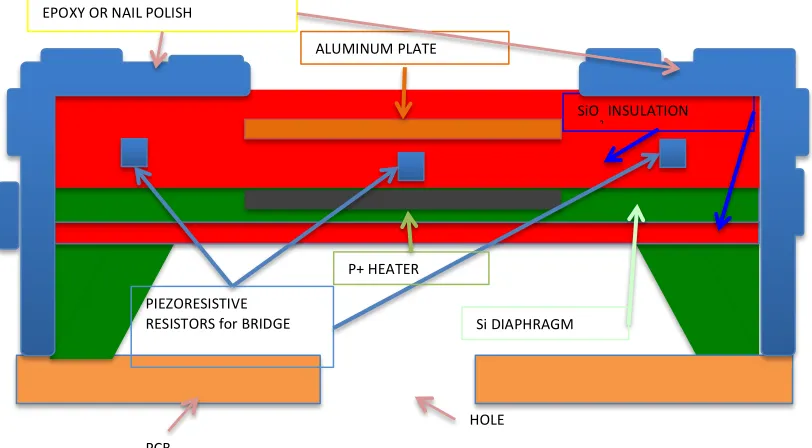
The device has been tested in different oil temperatures and compositions, for which viscosity measurements were taken. Taking the sensor to the next level leads to be able to measure viscosity in conductive liquids, because oil is a non-conductive medium it does not affect the sensors performance. But if a conductive fluid is present then everything changes, and the sensor stops working after a given period of time. Some of the problems encountered while testing the devices in conductive fluids are visible under a microscope by broken interconnects. The top layer of protection cracks due to pinholes that lead to the failure of the device. Thus the protective layer is very important when placing the sensor in conductive fluids.
Post processing fabrication of the protective layer has been chosen to be able to take advantage of all the existing viscosity sensors. At the same time this was chosen because if the fabrication steps were altered then the device would work at different specifications.
This is why many different MEMS-chips contain different packaging methods depending on the application that the sensor is going to be used upon. With this said, a new protective coating method will be
Poly
Resistors
Contact Pads
implemented and presented to the existing viscosity sensors. Afterwards they will be subject to test in order to find the corresponding viscosity measurements. All of these technological advancements have led MEMS to become a very sophisticated and useful technique to enhance various hi-technological devices, which are used throughout the entire world.
1.2.0 Micro-‐Electro Mechanical Systems
(MEMS)
& Biomedical-‐MEMS
(Bio-‐MEMS)
MEMS devices are known throughout the world because they are part of large components, various MEMS devices together produce a system. It is a link between the mechanical and electrical systems that operate together in a smaller scale. They have a variety of applications that are used today, in “the automotive industry, in process control and automation,
Figure 1.2 - NeoSense wafer with numerous MEMS devices [2]
scientific and medical instrumentation, telecommunication, commodity products, environmental monitoring, etc.” [3] With these broad applications this technology is advantageous for it has various uses in industry and affects people’s everyday life. The fascinations of using MEMS technology are its similar processes like the ones found in integrated circuit (IC) techniques [4]. Or the capability of mass production by using micro or nano scale devices on 4, 6, and 9-inch wafers (see Figure 1.2).
are composed of mechanical and electrical parts. Both parts together make a whole system, which is capable to move and give an electrical output, or vice-versa.
Figure 1.3 - Emerging MEMS market worldwide [5]
MEMS devices are very powerful and can be used to sense, feel, detect, or identify a specific problem, substituting our senses in case we are set to test something that is harmful to our well-being, or that we lack-of. With this said MEMS technology has increased in sales worldwide (see Figure 1.3) it is one of the best emerging technological markets in the world. At the same time companies can thrive to create jobs and enhance people’s everyday life [5,6].
Figure 1.4 – MEMS Pressure Sensor for automotive industry (left) [7] Bosch MEMS Digital Pressure Sensor (right) [8]
In electrical engineering there are many different sub-branches to study from. But the one most people are focused nowadays is the way MEMS technology proliferates by enhancing our life’s day after day. This can be seen in different recent devices, which some people call ‘electronic gadgets’: cellular phones, Nintendo Wii, Playstation 3, computers, monitors, Projectors (DLP), printers, mp3 players, etc.
sensors are located in the automotive industry, were pressure sensors [9] are found in seatbelts, airbag sensors, tires, etc. Figures 1.4 represent packaged MEMS pressure sensors for the automotive industry and the sensors size, respectively. In the end, it is thanks to these devices that help the driver and passengers to be safe at all times.
With this said MEMS sensors are implemented in many different ways to help the manufacturing industry in producing smaller sized devices, mass produce them, make them reliable, robust, and included in the latest technological gadgets. Similarly the cost of production is decreased because of these technological advancements. Going back to the idea of substituting our senses we can find that a relation to biology is very definitive. Researchers like to determine how to enhance solutions to problems every time new technologies are discovered. Thus the strong connection between MEMS and Biology happens to create a new branch of study named Bio medical micro electromechanical systems (Bio-MEMS).
Bio-MEMS like the name states is a relationship between biology, the study of life and MEMS, previously defined. Different applications can be seen being implemented in research in the industry of Bio-MEMS. Where there are currently two virtual ways in which the device is presented on the living body. One way of implementation is in-vitro (inside a living organism) where a sensor or device is inserted in the body being analyzed and works without harming it. Then we have in-vivo (outside the living organism) in which the sensor belongs to a contraption or device that uses the living tissue or fluid sample, removed from the body preventing from any harm, and tested in an isolated location.
1.3.0 Viscosity Sensors
Currently this project uses the device showed in Figure 1.1, a thermally actuated MEMS viscosity sensor [1]. The sensor is actuated by a thermal pulse, which then captures data regarding the deflection in the silicone membrane. With the data recorded, a set of mathematical equations is applied, and a computer interface is used to translate the data obtained to readable viscosity measurements. This can be seen from the read out values portrayed in the electronic portion of the sensor. The main focus on this project is the current problem with the application. It is based upon the use of non-conductive fluids, various kinds of oils with different viscosities. In order to improve this device it would be feasible to be able to use it on conductive fluids, such as milk, water, blood, etc. With this advantage the device will be able to be placed in substances that conduct electricity making it more practical to a Bio-MEMS perspective.
various types of viscometers, most of them are created by using simple and basic MEMS technology. They can be used to measure viscosity by using cantilever beams [10] [11] [12], resonating membranes [13] [14], or through quartz crystal resonators [15] [16] technology. The method implemented in the current sensor to measure viscosity is obtained by applying a pulse to obtain the resonating frequency within the testing liquid.
To obtain viscosity values using cantilever beams a deflection has to be applied to its beam. The beam will vibrate at its resonant frequency, becoming a useful value that relates to viscosity. As the beam exerts a deflection it is recorded using resistors, the most common way is to use a wheatstone bridge setup which measures the voltage difference. This is taken into account and the result is the characteristic properties of the fluid, which will correspond to measurements of viscosity. An application in which this type of viscometer is used involves a semi-permeable membrane that encloses a vibrational cantilever beam for glucose detection [10].
Figure 1.5 - MEMS Glucose Monitoring System [10]
In the picture above, Figure 1.5 a schematic of a MEMS glucose sensor is visible showing the cantilever beam enclosed with a semi-permeable membrane so that only the glucose solution is able to penetrate it. The polymer solution, which is located inside the chamber, contains Dextran and Con-A. Inside it cross-linking occurs between both solutions meaning that their physical properties change, forming a viscous mixture. As glucose enters the chamber through the membrane the molecules bind with Con-A since it is a glucose binding protein and this reaction weakens the Dextran – Con-A crosslinking relationship. As this occurs the mixture becomes less viscous and increases the dampening on the vibrating beam, helping determine glucose concentrations from the vibration values [10]. With the vibration characteristics it is possible to relate them to viscosity measurements. Zhao et al determined that their sensor works for frequencies under 2,000 Hz inside the solution.
making them suitable for capturing viscosity measurements by applying the principle of vibrating plates. Some of their results are visible in different sugar solutions presented in Figure 1.6.
Figure 1.6 - Results from viscosity sensor of Frequency and Q Factor in different sugar solutions [11]
Vibrational type viscometers are another kind that is used in industry. In this case in order to obtain viscosity at least three different measurements are required. These are the amplitude, resonant frequency and the quality factor. By understanding how these three measurements behave a viscosity reading can be obtained.
2.0 Thermally Actuated Viscosity Sensor
2.1.0 Electrical Components
With the layout of the design shown in Figure 1.1, it is possible to separate the device in two processes. The first one involves a heater, and the second one a wheatstone bridge circuit.
2.1.1 Heater
The first device implemented in this sensor is the heater. Basically the heater is designed from a Polysilicon resistor. The resistance in Figure 6 is determined from the sheet resistance of the material. In this case, the material is Polysilicon, and its measurement depends on the size of the resistor, which is obtained from the length divided by the width, see Eq. 2.1.
Figure 2.1 - Heater circuit schematic
𝑅= ρ!
L
𝑊 (2.1)
Overall the heater works from the process of joule heating, which involves an applied current going through a resistor and releasing heat, or producing power (see Eq. 2.3). James Prescott Joule first introduced this in 1841 with an experiment involving a long wire with a specific volume of water and measured the temperature change with respect to the current that was flowing through the wire for a period of roughly 30 minutes[19]. Out of his experiment he was able to come up with an assumption that the heat produced, Q, is proportional to the square of the current, I, flowing times the electrical resistance, R, of the material of the wire [19]. This is known as Joule’s First Law (see Eq. 2.2).
𝑄∝𝐼!∗𝑅 (2.2)
I
RH = ρs (L/W)
ρs = Sheet Resistance
L = Length
W = Width
+
At the same time we know that due to an involvement between the voltage drop and the current traveling through, the resistor produces an amount of energy per time measured in (Joules/seconds). This output of power, also measured in Watts is able to convert the electrical energy to a thermal energy through the release of heat, which is found in the following Eq. 2.3.
𝑃=𝑉𝐼=𝐼!𝑅 (𝑊𝑎𝑡𝑡𝑠) (2.3)
The heater will be used to activate the diaphragm and help it resonate at a given frequency in this case its natural frequency. This depends on the voltage applied to the heater.
2.1.2 The Wheatstone Bridge Circuit
We then have the second process, which involves the wheatstone bridge circuit. Sir Samuel Hunter Christie invented this design in 1833 and Sir Charles Wheatstone enhanced it and revolutionized it in 1843 [20], [21] he used the device to be able to analyze and compare the results from different soils. The main purpose of the wheatstone bridge is defined as a ‘differential resistance measurer’, used to distinguish the resistance for an unknown value on one of the branches. Below is an overview of a design of a wheatstone bridge circuit.
Figure 2.2 – Wheatstone bridge Design [20], [21]
Normally R4 would be the unknown resistance value, but this depends on the users approach. In the case R4 is the unknown value, assumptions are made, first we have to balance the entire circuit, it occurs when:
R
1
R
2
R
3
R
4
Δ
V
output
V
s
GND
∆𝑉=𝑉!−𝑉!=0 (2.4)
𝑉!=𝑉! (2.5)
Then the circuit gets analyzed using Kirchhoff’s Current Law (KCL), shown in Eq. 2.6 where the sum of all currents going in are equal to those leaving a node. By applying this law and assessing just like shown in Figure 2.3:
Figure 2.3 – Wheatstone bridge Design used for analysis
𝐼! =0
!
!!!
(2.6)
where k represents the nth number of nodes, and n is the total number of currents going in or leaving the node in question. Above in Figure 2.3,by analyzing the nodes in V1 and V2 we find:
At Node V1 we have: 𝐼!−𝐼!−𝐼!"#$"#=0
Or 𝐼!=𝐼! assuming 𝐼!"#$"#=0 (2.7)
At Node V2 we have: 𝐼!−𝐼!+𝐼!"#$"#=0
Or 𝐼!=𝐼! assuming 𝐼!"#$"#=0 (2.8)
Now applying Kirchhoff’s Voltage Law (KVL) shown in Eq. 2.9 it is possible to find a couple of voltages from every resistor and given currents. So applying this at nodes V1 and V2.
𝑉! =0
!
(2.9)
R
1
R
2
R
3
R
4
Δ
Voutput
V
s
GND
V
1
V
2
I
1
I
3
I
4
I
2
I
out
Using Ohm’s Law:
𝐼=𝑉
𝑅 →𝑉=𝐼𝑅 (2.10)
At Node V1 we have: 𝐼!𝑅! − 𝐼!𝑅! − 𝐼!"#$"#𝑅!"#$"# =0 (2.11)
At Node V2 we have: 𝐼!𝑅! − 𝐼!𝑅! + 𝐼!"#$"#𝑅!"#$"# =0 (2.12)
Now that the circuit is balanced, assuming the bridge gets balanced, thus Voutput≈ 0, will give a Ioutput≈ 0 amperes. Both sets of new equations are placed equal to each other just like Eqs. 2.13 and 2.14 which satisfy the assumption from Eqs. 2.7 and 2.8:
𝐼!𝑅! − 𝐼!𝑅! − 0 =0
𝐼!𝑅! − 𝐼!𝑅! =0
𝐼!𝑅! = 𝐼!𝑅! (2.13)
𝐼!𝑅! − 𝐼!𝑅! + 0 =0
𝐼!𝑅! − 𝐼!𝑅! =0
𝐼!𝑅! = 𝐼!𝑅! (2.14)
Now look for the value of R4 by setting Eqs. 2.13 and 2.14 equal to each other:
𝐼!𝑅! 𝐼!𝑅! = 𝐼!𝑅! 𝐼!𝑅! (2.15)
𝑅!= 𝐼!𝑅! 𝐼!𝑅!
𝐼!𝑅! 𝐼! (2.16)
Using the KCL assumptions from Eqs. 2.7 and 2.8
𝐼!=𝐼! and 𝐼!=𝐼! (2.17)
R4 can be reduced to resistor values:
𝑅!=
𝑅! 𝑅!
𝑅! (2.18) With the known values of R1, R2, and R3 it is possible to calculate the value of R4 when this type of electrical circuit is chosen.
device. This can be obtained in the following form from Figure 2.2 and knowing the previous mathematical explanation:
𝑉!"#$"#=𝑉!−𝑉! (2.19)
𝐴𝑡 𝑛𝑜𝑑𝑒 𝑉!=
𝑅!
𝑅!+𝑅! 𝑉! (2.20)
𝐴𝑡 𝑛𝑜𝑑𝑒 𝑉!=
𝑅!
𝑅!+𝑅! 𝑉! (2.21)
Substituting the known values with their respective coefficients:
𝑉!"#$"#=
𝑅!
𝑅!+𝑅! 𝑉!−
𝑅!
𝑅!+𝑅! 𝑉! (2.22)
𝑉!"#$"#= 𝑅!
𝑅!+𝑅!
− 𝑅!
𝑅!+𝑅!
𝑉! (2.23)
Obtaining the relative voltage output at given nodes V2 and V1.
For purposes of this sensor, the style of circuit used is very similar to the one presented in Figure 2.2, which shows four resistors arranged as two parallel branches with two resistors in series in each branch. A voltage difference can be recorded through the use of two probes on nodes V1 and V2, the opposite sides from where the +5V (Vs) and ground (GND) connections are found. The main purpose for this circuit is to be able to measure the voltage difference found in the stress of the resistors as the diaphragm vibrates, this in other words is the measurement of the root mean squared (RMS) of the voltage difference.
The voltage is sensed by the resistors, which happen to be located where most of the stress occurs on a diaphragm.
The image above relates the dimensions used in the sensors. This simulates the stress locations on the diaphragm (purple) and is a suitable way to help place the resistors (red) on these exact locations where most of the stress is located, similar to various square pressure sensors.
After producing the pulse from an Agilent 33220A signal generator the voltage send from the power supply goes through the heater, activating the diaphragm and goes into a power MOSFET STP12PF06. The power MOSFET is used as a switch for the current to go through, an overview of how it is used is shown below.
Figure 2.5 – Heater and Power MOSFET schematics
After the power MOSFET comes the instrumentation amplifier INA101HP (see Figure 2.6), this IC is used as a signal amplification for the wheatstone bridge or strain gauge. It comes packaged in a dual in line (DIP) mode, and easy to apply to a printed circuit board (PCB). This amplifier was chosen because it contains three operational amplifiers, which are designed to obtain high-accuracy general purpose data and produce a low level signal amplification.
Figure 2.6 – Instrumentation Amplifier (INA-101HP)
Figure 2.7 – Instrumentation Amplifier Circuitry (INA-101HP) [22]
Figure 2.7 above represents the circuit layout of the instrumentation amplifier. In the picture there is a section where a resistor, RG is connected near the Gain Set 1 and 2 that is a potentiometer used to increase or decrease the gain from the sensors output. In order to power the IC it requires ±12V to go in to the device, applying that exact amount to pins 2 and 13 and common ground is connected through pin 14. The two input signals going into this IC are V1 and V2 each one goes to pins 3 and 12 correspondingly. These represent the voltages at the nodes between the resistors and due to the stress where the location of the resistors are situated it is possible to obtain a
voltage difference. Which also represents the deflection according to the voltage difference; this is calculated from a specific set of equations. Since the voltage output from the bridge is relatively small, it requires to get amplified in order to accurately obtain a specific deflection this is applied thanks to the use of operational amplifiers. The output measuring the deflection shown as a sinusoidal wave is obtained from pin 1 and it is send to the oscilloscope (Tektronix TDS 340) which portrays the signal, just as shown below in Figure 2.8.
Figure 2.8 – Example of Output from a Sensor in Glycerol-Water Mixture
2.2.0 Physical Components
The thermally actuated viscosity sensor behaves like a powerful device because it can determine the viscosity of the liquid. The sensor is CMOS compatible and uses MEMS technology in order to achieve exceptional
performances previously stated. The production price to build the device is relatively inexpensive and it can be produced in massive quantities. At the same time the device is reliable and the measurements are taken electronically in order to determine the viscosity of the fluid. This device uses the principles of vibration plates, which in turn is based upon the readings obtained and then this data is translated to values easy to understand. In order to produce a thermal signal on the sensor, a heat pulse is produced. Mathematically, what happens to the diaphragm (see figure 2.9) as it moves up and down in the Z axis can be seen in the following Eq. 2.24:
𝑧= ℎ
Figure 2.9 – Diaphragm on XYZ Coordinate to Define Direction of Deflection [23]
Where z represents the Z-axis found in the coordinate system of a diaphragm, and h is the thickness of the plate. With this equation we can see that after heat is applied, temperature is also applied as a side effect because the diaphragm will be in motion exerting molecules to move back and forth. Due to the side effect temperature will effectively change over time. Together with this a solution is presented in [23] where the vertical direction (z) is where most of the deflection of a square membrane occurs. Different equations were obtained in order to understand the behavior of the plate, therefore it was determined that the plate would have static and dynamic solutions that would depend on the step heat input applied. [23] In this case this direction is denoted as w and is represented in the following Eq. 2.25:
𝑤 𝑥,𝑦,𝑡 =𝑤!"−𝑤!"# (2.25)
Where Wst and Wdyn represent the static and dynamic terms respectively. By introducing the dynamic and static solutions as a time dependent equation we can obtain Eq. 2.26, which will be used to obtain the angular frequency of oscillation for the diaphragm, the study from [23] led to a relationship of:
w!=!!
!
!!
!!!
!"!!!!
!! (2.26)
a
h
Where a is the length of the plate, h is the thickness of the plate, 𝜌 is the density of the material, E is Young’s Modulus, and v is Poisson’s Ratio. Figure 2.10 gives an overview of some of the measurements required to calculate angular frequency.
With this equation it can be assumed that the sensor operates only if there is a fast enough heat pulse implemented. Without it the sensors response will be null and no output will be obtained. Luckily a heat pulse was chosen instead of step heating because this would not affect the fluids temperature. Thus it is vey important for the fluid to not change temperature while testing, because viscosity is dependent upon the temperature. With this reaction the device would act correctly and the electronics attached would obtain the data. An important point to know from this sensor is that the thermal properties do not affect the frequency of oscillations [1]; keeping the device in a more controlled environment.
Dr. Puchades also found that time is dependent upon the heat pulse produced. This can be seen on the following graph Figure 2.11 which states how temperature is affected by the pulse time.
Figure 2.11 - Temperature Increase of a Membrane in Air and Oil for Pulsed Heating [1]
𝑄=2𝜋 !"!#$!!"#$%&
!"!#$!!"##"$%&'!!"! !"!#$
≈!.!"
! 2.27
𝜉= 𝑣
𝑤𝑎! (2.28)
Where 𝑣, represents the kinematic viscosity, w is the radial frequency of vibration, and a is the radius of the membrane. With these factors the density and the viscosity of the liquid can be calculated [1]. Overall the natural frequency of vibration for a simple square thin plate in air can be determined from the following equation [27]:
𝑓!"!=
19.74
2𝜋𝑎!
𝐸ℎ!
12𝜌ℎ 1−𝑣!
! !
(2.29)
Where a is the length of the plate, E is Young’s Modulus, 𝜌 is the density, h is the thickness of the plate, and v is Poisson’s ratio.
As a matter of fact the overall design of the interaction between the fluid and the plates involves the density and viscosity of the fluid. It starts as an analysis by Horace Lamb in 1920, when his experiment proved that a circular plate oscillating in water produces vibrating modes that are very similar. But there is a slight variation in the frequency response from the vibrating waves, he denotes this feature as β calling it an added virtual mass [26]:
𝑓!"#$%= 𝑓𝑎𝑖𝑟
1+𝛽 (2.30)
Lamb found that there is a relationship between the frequency of the fluid, 𝑓!"#$%, and the frequency in air,
𝑓!"#. They both depend upon the density of the fluid, 𝜌!"#$% , the density of the material used for the plate, 𝜌!"#$%, the
radius a, and thickness h of the plate. The outcome is that he took into account the slight variation and applied it as an equation [26].
𝛽=0.669!!"#$%!
!!"#$%! (2.31)
the system that depends on the kinematic viscosity, 𝑣, which stands for the ratio between the dynamic viscosity, η, and the density, ρ, just like previously explained Eq. 2.28.
𝛽=0.6538!!"#$%!
!!"#$%! 1+1.082𝜉 (2.32) The electrical components that operate in this device are used to relate the data gathered to analyze and compare the expected results. The results are used to determine the Q factor. They require some signal amplification in order to analyze and understand what the collected data means. In this case the output signal is an oscillating curve that is represented from the deflection of the membrane, and the values correspond to the change in voltage of the Wheatstone bridge.
Figure 2.12 -‐ FFT for Device 1P, Used to Determine Q [1]
A Fast Fourier Transform (FFT) is used with LabView because the graph shown with the data obtained from the signal needs to be revised and analyzed to produce a Q factor and frequency values. For the frequency the peak value is recorded from Figure 2.12, and Q is calculated using Eq. 2.33 were the values are also dependent on the signal output.
𝑄= 𝐹!
∆𝑑! (2.33)
Figure 2.13 -‐ Normalized Frequency and Q Factor Versus Kinematic Viscosity and Temperature [1]
3.0 Testing of Existing Viscosity Sensor with packaging method Version 1
Currently there are two signals used to make the sensor operate, one activates the diaphragm and the second one is the actual output the sensor produces. There are two main designs in this device; they are both previously explained in Section 2.0 Thermally Actuated Viscosity Sensor. Consequently the device is ready for testing and these are the primary results from the experiment.
3.1.0 Screening Experiment
Initially four wafers were obtained from previous testing, and devices with passivation were searched and removed from the diced wafers. This process was named the screening experiment because it had the purpose to identify all working devices. This was done very meticulously, all the new devices got named and tested to make sure they worked to specifications. All resistors were operational and the gathered devices had a properly balanced wheatstone bridge. Each die was tested under a 5V power supply to measure the voltage difference from the resistors in the wheatstone bridge. A ohmmeter was used to make sure the
Figure 3.1 - An Overview of How the Devices were Tested
heater had a resistance value and their were no open circuits within the sensor. See Figures 3.1 and 3.2 for the visual schematics and electrical circuits of how the devices were being tested for future reference.
For these tests the Agilent 33401A was used as the digital multi-meter (DMM), and at the same time the device was placed in the testing probe to hold the device and provide a vacuum on the back to keep the device from moving from side to side as test probes were lowered. Testing probes were placed on top of the device were the
DMM V1 2.487 V Power
Supply +5V
DMM 270.50 Ω DMM V2
2.621 V
GND V2
contact pads were located, at first this was hard to appreciate, but after testing a lot of devices lowering the probes to the contact pads became a habit. The DMM was connected in parallel in order to measure the resistance of the heater. On the second type of test a power supply was used providing +5 volts to the bridge in order to obtain the different voltage readings from the device, and be able to calculate the change in voltage between V1 and V2. At V1 and V2 two different DMM’s were used to measure the voltage reading by connecting the negative side to ground and the positive to the corresponding pad just like shown above in Figure 3.1.
Figure 3.2 – Electrical Schematic of the Wheatstone Bridge
These measurements were compiled in a table together with the material of the resistors and the size (see Appendix for table 1A) and used later for reference. An example of the measurements taken for one device is shown in the following Table 3.1.
Table 3.1 - Example of measurements obtained from a single die from Wafer 3
Each die was placed in a new empty box container in order to choose from for later use and organize them according to the wafer each of them came from. This was very important because there were initially four wafers to choose die from. Wafers 3 and 4 contained die with a diaphragm thickness of 15µm. Wafer 5 contained devices with a thickness of 10µm and all of Wafer 6 had a thickness of 6µm. The first column defines the number given to the device, which was placed inside the box with the rest of the devices and would help differentiate them from each other.
Device
# a-Size (mm)
Details
Resistor Type (P+ /
Poly)
Resistor Size (35%, 16%,
2%) Metal? Rheater (Ω)
VBridge
(mV)
Every numbered device had a second set of characteristics, which defined the length of the membrane or a-size ranging from 1 mm, 1.75mm to 2.5mm. At the same time each die had a specific heater resistor type and a-size. The material that the resistor was made out of for the heater varied between P+ Diffused or Poly. Another important factor that changed from each die was the size of the heater covering the area around the diaphragm ranging from 2%, 16% to 35%. Puchades previously analyzed the differences between each of the type of heaters in [1] concluded that the heaters with P+ diffused heaters and their respective resistor size, whether 2%, 16% or 35% bended the membrane downwards by 10 µm. If Polysilicon were used instead then the membrane would move that same amount in the opposite direction, regardless of the size between 16% and 35%. Where as for a Polysilicon heater with a resistor size of 2% would bend the diaphragm down just like a P+ diffused heater.
The other important column was the one containing Metal, even though some die had metal and others didn’t the overall conclusion for the presence of metal was noticed in [1]. The different observed results shows that there is a variation in the quality factor, sensors with metal on top have a higher value. On the other hand the ones that did not have metal contained a lower value. The two last values on the table refer to the values obtained from testing both setups previously explained in this section.
All of these values were recorded in a excel spreadsheet and tabulated for later use, see Table 3.2 below for a section of the file.
Table 3.2 - Devices 1 Through 10 with Characteristics from Wafer 3
Details
Device #
a-Size (mm)
Resistor
Metal Rheater (Ω) V
(mV)
BridgeType (P+ /
Poly) Size % (2, 16, 35)
1
1.75
P
2%
Yes
60
78.7
2
1
P
35%
No
217
12.8
3
1
Poly
2%
Yes
46.7
35.7
4
1
Poly/P+
2%
Yes
52
11.5
5
1
Poly
16%
Yes
70
95.7
6
1
Poly
1%
No
100
-16.7
7
1
P
2%
Yes
309
30.5
8
1
P/P+
2%
No
267
1.105
9
1
Poly
2%
No
90
-50.7
Later in the experimentation section these values would help determine reasons for failure in the underwater tests with the existing packaging. Each of these thicknesses is used in Eqs. 2.26, 2.29, and with them it is possible to calculate a different resonant frequency. Overall the device will output signals that vary depending on the material dimensions. Table 3.4 gives an overview of the calculated frequencies for the sensors in air, depending on their dimensions.
3.1.1 Calculating the frequency in Air
Just like previously stated the frequencies in air were calculated from equation 2.26 or 2.29 depending on the units, either radians per second or cycles per second correspondingly. The equation is very simple once all the variables are obtained, assuming we have a die from wafer 3 with the following parameters shown in Table 3.3:
Table 3.3 - Measurements to Calculate the Frequency in Air of a Device from Wafer 3
h, thickness of membrane
a, length of membrane
E, Si Young's Modulus
v, Poisson's
Ratio
ρ, Density of Si
15𝑥10!! 𝑚 1.75𝑥10!! 𝑚 1.9𝑥10!! !
!! 0.3 2330
!" !!
𝑓!"#=
19.74
2𝜋∗1.75!
𝐸∗0.000015!
12∗2330∗0.000015∗ 1−0.3! !
!
(3.1)
𝑓!"#=42,050 𝐻𝑧 (3.2)
With this said, this assumes that the measurements are all perfect and nothing went wrong during fabrication or packaging processes. Thus a sensor with these characteristics will output a response of 42,050 Hz in air. Similarly this can be done to the rest of the devices that have different characteristic properties and Table 3.4 shows the output response expected from them. Consequently a column gets added to the data in Table 3.1 for the calculated value of the frequency in air of each device and look just like Table 3.5.
Table 3.4 - Calculated Frequencies in Air at a Given Thickness and Length Size, a
Calculated FAir (Hz)
a (mm)
1 1.75 2.5
h(µm)
15 128,779 42,050 20,605 10 85,853 28,034 13,736
Table 3.5 - New Column Added to Table 1 with Calculated Frequency in Air Value
Device # Details a-Size (mm) Heater
Metal Rheater (Ω) V(mV) Bridge Calculated F
Air (Hz)
Resistor Type (P+ / Poly)
Resistor Size (35%, 16%, 2%)
1 1.75 P 2% Yes 60 78.7 42,050
With the value of the calculated frequency a time period can be deduced, and this information will be used to determine the heat pulse applied to the sensor. Sending this pulse to the device causes the membrane to vibrate at its resonant frequency producing an oscillating wave. The oscilloscope will be able to view this output, which in turn is recorded by the computer interface, in this case LabView. As the device changes medium from air to a fluid a variation will be witnessed. A frequency change is expected as the medium changes and the Q factor varies with the frequency accordingly. This can be seen in Eq. 2.29, which contains information regarding air, and Eq. 2.30 has a different calculation for the frequency in a fluid.
3.1.2 Calculating the frequency in a Fluid
To be able to determine the frequency of the device on a given fluid a different equation was applied. In this case Eq. 2.30 previously described in Section 2.2.0 is used to be able to determine the frequency, this equation is completely different because it involves the previous Eq. 2.29 to determine the frequency in air with another term, which is previously explained in Section 2.2.0 as β. Consequently the new term involves the density of the fluid, the length of the membrane, the density of the material of the diaphragm, and the thickness of the membrane. With all of these values it is possible to find the frequency of the fluid assuming all measurements are accurate enough to be used for the simulations.
From previous calculation for the frequency in air of a sensor we are able to solve the first part of the equation. As for the second portion we input the next set of parameters:
Table 3.6 - Parameters to Calculate the Frequency of the Sensor in a Fluid
h , thickness of diaphragm
a , length of membrane
E , Si Young's Modulus
v , Poisson's
Ratio
ρ of plate , Density of Si
ρ of fluid, Density of DI
water
15𝑥10!!𝑚 1.75𝑥10!!𝑚 1.9𝑥10!! !
!! 0.3 2330
!"
!! 1000
With these new parameters it is possible to calculate the frequency of the sensor in a given fluid, in this case we are using distilled water as the fluid. The calculations goes as follows for a device with an a = 1.75 mm, and an h = 15 µm:
𝑓𝑎𝑖𝑟=42,050 𝐻𝑧
𝛽=0.669(1000∗1.75𝑥10!!)
2330∗15𝑥10!! =33.497854
𝑓!" !"#$%=
42,050
1+33.497854
𝑓!" !"#$%=7,159.3 𝐻𝑧
A sensor with these measurements will theoretically produce a resonant frequency of 7,159 Hz inside a vial of de-ionized water.
3.1.3 Determining the L2T and Pulse Time for good output
A way to determine the best die for this project is to choose the correct diaphragm thickness and side length for the sensor. This will allow calculating a ratio between both values. This ratio will then be used to determine the best die that will provide the correct dimensions and avoid any side effects from the materials used. In a study by Brand e.t. al, it was proven that sensors with a ratio higher or lower than 166 would produce non-linearity effects, and tend to limit the output produced by the sensors. This ratio is used to avoid any non-linearity effects found from material stiffening, membrane buckling from compressive stress [29]. The sensors tested would not be working to their full capability and this value was used to compare the different expected results from different thicknesses and side lengths. The approximate value used to achieve the perfect ratio is ≈166 [29,14], which means that the critical thickness to length ratio calculated should be close to 166.
If the hand calculations agree with the pre-determined value of 166, then it is possible that there will be fewer side effects present as the membrane vibrates for the provided dimensions. These values can also be found on a modified Table 3.1, shown in the last column length to critical thickness ratio (L2T) as seen below.
Table 3.7 – Length to Critical Thickness Ratio Column
Device # Details a-Size (mm) Heater
Metal Rheater
(Ω)
VBridge (mV) Fair (Hz) L2T Ratio Resistor Type
(P+ / Poly)
Resistor Size (35%, 16%, 2%)
As for the length to critical thickness ratio, there are die with similar and dissimilar dimensions meaning there will be different values that are higher and lower than 166, while others would contain similar ratios. This operation is done by applying Eq. 3.3 from [29], where a is the length size of the membrane, and h is the thickness of the membrane, these measurements can be seen in Figure 2.9.
𝐿𝑒𝑛𝑔𝑡ℎ 𝑡𝑜 𝑇ℎ𝑖𝑐𝑘𝑛𝑒𝑠𝑠 𝑅𝑎𝑡𝑖𝑜= 𝑎 (𝑚𝑚)
ℎ (µμ𝑚) (3.3)
With Eq. 3.3, the best die can be chosen from the screening experiment and this helps by determining the best device in our samples. This is also very important because it can avoid non-linearity or buckling effects [14]. From this explanation each device from their corresponding wafer was evaluated and the best ones were chosen for testing. Wafers 3 and 4 contain the same membrane thickness, h of 15µm. Even though each wafer had many devices with different lengths, an a of 2.5mm was chosen because the calculated ratio was 166.7 which matches the desired thickness to length ratio. Just like previously stated, a value ≈166 is the best value for non-linearity effects. The same approach was taken to determine the best die in wafers 5 and 6. For wafer 5 it was established that the best length size was 1.75mm for a thickness of 10µm, since the ratio obtained from these measurements was of 175. Even though it was off by a value of 9 units from the target value, this was close enough to the desired value, compared to the rest of the calculations. For wafer 6, the best die was determined to be those with a thickness of 6µm and a length size of 1mm, giving a value of 166.7. But this would also mean that it is the smallest length size available and diaphragm thickness, thus it should be harder to see the oscillations produced by the sensor. Table 3.7 explains the different calculations for each of the sensors according to their h and a values.
Table 3.8 - Information on L2T Ratios for all the Different Devices
Wafer h(µm) a(mm) L2T
3, 4 15 1 66.7
Too Far from desired L2T
1.75 116.7
Near desired L2T
2.5 166.7
Close or perfect match for L2T
5 10 1 100.0
1.75 175.0
2.5 250.0
6 6 1 166.7
1.75 291.7
2.5 416.7
Desired Length to Thickness Ratio for less non-linearity effects h = 15µm à a = 2.5mm (Wafers 3, 4) L2T = 166.7
After the screening process, each device was tested in air. This was done to show that the device would work close to an expected calculated value and produce the output signal. The calculated frequency obtained from Eq. 2.29 would help find its resonant frequency by applying the value to the following Eq. 3.4 to find the time period.
𝑓=1
𝑡 (3.4)
𝑓!"#!$#"%&'=
1
𝑡!"#!$#"%&' (3.5)
where 𝑓!"#!$#"%&' is the frequency calculated in air, and 𝑡!"#!$#"%&' is the calculated time period
𝑡!"#!$#"%&'=
1
𝑓!"#!$#"%&' (3.6)
Once the time period is found, this value would be applied to the heater. This would help determine the pulse required for the membrane to resonate at its natural mode of vibration. Sometimes the calculations did not provide an adequate time, and caused delays in obtaining the results by requiring a trial and error approach. One of the main reasons for this to occur was due to the fabrication steps. Depending on the pre-determined times of RCA cleans and wet etch baths, the step could be done under the given amount of time, right at the spot, or a little over. There is always some space for error, and while fabricating these devices, these changes are taken into account because it can always damage the end product. Table 3.8 shows the time required for the heat pulse to be ON in order for the sensor to vibrate at its resonant frequency.
Table 3.9 - Time Required for Heat Pulse to Activate Sensor
Device # Details a-Size (mm) Heater Resistor
Metal Rheater
(Ω)
VBridge (mV) Fair (Hz) L2T Ratio Time (µs) Type
(P+ / Poly)
Size (35%, 16%, 2%)
1 1.75 P 2% Yes 60 78.7 42,050 116.7 23.8
Next is the pulse width, which is determined from the frequency in air calculation or Eq. 2.29. This value is used to determine the time period required to input the pulse from Eq. 3.6. In this case the pulse is applied using an Agilent 33220A Signal Generator. With this device it is possible to input a pulse at a frequency of 5 Hz, this also means that the signal send is always OFF and it will be ON only for a short period of time, with a range from 0V -5V. Figure 3.3 explains the signal generators output.
Figure 3.3 - Graph Showing Pulse from Signal Generator
After the frequency a