Self-localization in ubiquitous computing using sensor fusion

(1)

Rochester Institute of Technology

RIT Scholar Works

Theses Thesis/Dissertation Collections

11-15-2006

Self-localization in ubiquitous computing using

sensor fusion

Jeffrey Zampieron

Follow this and additional works at:http://scholarworks.rit.edu/theses

This Thesis is brought to you for free and open access by the Thesis/Dissertation Collections at RIT Scholar Works. It has been accepted for inclusion in Theses by an authorized administrator of RIT Scholar Works. For more information, please contactritscholarworks@rit.edu.

Recommended Citation

(2)

Self-Localization in Ubiquitous Computing using Sensor

Fusion

by

Jeffrey Michael Domenic Zampieron

A Thesis Submitted in Partial Fulfillment of the Requirements for the Degree of Master of Science in Computer Engineering

Supervised by

Dr. Juan C. Cockburn Associate Professor Department of Computer Engineering

Kate Gleason College of Engineering Rochester Institute of Technology

Rochester, New York November 2006

Approved By:

Associate Professor Dr. Juan C. Cockburn Primary Adviser

Dr. Shanchieh Jay Yang

Assistant Professor, Department of Computer Engineering

Dr. Roxanne Canosa

(3)

Thesis Release Permission Form

Rochester Institute of Technology

Kate Gleason College of Engineering

Title: Self-Localization in Ubiquitous Computing using Sensor Fusion

I, Jeffrey Michael Domenic Zampieron, hereby grant permission to the Wallace

Memo-rial Library reporduce my thesis in whole or part.

Jeffrey Michael Domenic Zampieron

(4)

c

Copyright 2006 by Jeffrey Michael Domenic Zampieron

(5)

Dedication

This thesis is dedicated to my Mother and Father for their countless reminders, support and

(6)

Acknowledgments

I would like to acknowledge each of my committee members for their contributions to this

work. They have been invaluable assets as both experts in their fields and as proofreaders.

Additionally, I would like to acknowledge Professor Bruce Hartpence from the

Depart-ment of the Networking, Security, and Systems Administration in the Golisano College of

Computing and Information Sciences (GCCIS) for his insights into some of the issues with

(7)

Abstract

The widespread availability of small and inexpensive mobile computing devices and the

desire to connect them at any time in any place has driven the need to develop an accurate

means of self-localization. Devices that typically operate outdoors use GPS for

localiza-tion. However, most mobile computing devices operate not only outdoors but indoors

where GPS is typically unavailable. Therefore, other localization techniques must be used.

Currently, there are several commercially available indoor localization systems. However,

most of these systems rely on specialized hardware which must be installed in the mobile

device as well as the building of operation. The deployment of this additional infrastructure

may be unfeasible or costly.

This work addresses the problem of indoor self-localization of mobile devices without

the use of specialized infrastructure. We aim to leverage existing assets rather than deploy

new infrastructure.

The problem of self-localization utilizing single and dual sensor systems has been well

studied. Typically, dual sensor systems are used when the limitations of a single sensor

prevent it from functioning with the required level of performance and accuracy. A second

sensor is often used to complement and improve the measurements of the first one.

Some-times it is better to use more than two sensors. In this work the use of three sensors with

complementary characteristics was explored.

The three sensor system that was developed included a positional sensor, an inertial

sensor and a visual sensor. Positional information was obtained via radio localization.

Acceleration information was obtained via an accelerometer and visual object identification

(8)

ubiquitous computing devices that will be capable of developing an awareness of their

environment in order to provide users with contextually relevant information.

As a part of this research a prototype system consisting of a video camera,

accelerom-eter and an 802.11g receiver was built. The specific sensors were chosen for their low cost

and ubiquitous nature and by their ability to complement each other in a self-localization

task using existing infrastructure.

A Discrete Kalman filter was designed to fuse the sensor information in an effort to

get the best possible estimate of the system position. Experimental results showed that

the system could, when provided with a reasonable initial position estimate, determine its

(9)

List of Figures

1.1 Sensor System Environmental Interaction Diagram . . . 9

3.1 Camera Coordinate Frame([22],379) . . . 16

3.2 Line Projection onto Unit Sphere([19],2) . . . 17

3.3 Camera Distance Model . . . 18

3.4 A Detected Door Lock . . . 20

5.1 System Setup . . . 28

5.2 System Block Diagram . . . 30

6.1 Accelerometer with 68HC12 Interface . . . 40

6.2 Cannon VC-C4 Pan/Tilt/Zoom S-Video Camera . . . 41

6.3 AVerMedia AVerTv Cardbus Frame Grabber . . . 42

6.4 The Accelerometer Display . . . 45

6.5 OpenCV’s Extended Haar Feature Set[13] . . . 49

6.6 Example Positive Image . . . 50

6.7 Example Positive Image, Sobel filtered, Door Lock Marked . . . 51

6.8 Example Negative Image . . . 52

6.9 Example Negative Image, Sobel filtered . . . 52

6.10 Classifier Feature Count per Stage . . . 53

6.11 Wireless Distance Model . . . 56

6.12 System Controller Window . . . 58

7.1 System Model Step Response . . . 73

(13)

List of Tables

3.1 Camera Model Raw Data . . . 19

6.1 Haar Classifier Cascade Feature Counts . . . 54

6.2 Wireless Strength vs. Distance . . . 55

7.1 Stationary Aggregate Data . . . 67

7.2 Movement Aggregate Error Statistics . . . 68

7.3 Movement Trial 2 Error Statistics . . . 69

(14)

Glossary

B

Bluetooth A short range low power RF hardware/software standard meant for embed-ded devices., p. 81.

D

DGPS Differential Global Positioning System. A positioning system which uses GPS

but with better accuracy. The accuracy of the system is enhanced by the use of

ground based transmitters at precisely known locations., p. 84.

E

EKF Extended Kalman Filter. A form of the Kalman filter where the Q and R

matri-ces are non-constant. The system is point linearized and the error covarianmatri-ces

are updated at each time step., p. 80.

G

GPS The Global Positioning System. A system deployed by the United States

De-partment of Defense to provide latitude and longitude information from

(15)

I

INS Inertial Navigation System. The use of heading and motion from within a

sys-tem to determine the position and frequently the heading of the syssys-tem., p. 81.

R

RSSI Received Signal Strength Indication. A measurement of the intensity of an RF

signal. The measurement is taken at the receiving end., p. 12.

S

SMT Simultaneous Multithreading. The use of a execution units on a single

micro-processor core by multiple concurrent threads., p. 60.

T

TDOA Time Delay of Arrival. A technique for calculating distance between a

trans-mitter and receiver based on the time required for data to travel between the

two points., p. 82.

U

UWB Ultra-Wide Band. A class of networking devices that use a large frequency

spectrum to deliver very high speed RF communications over short ranges.,

p. 82.

W

(16)

Z

(17)

Chapter 1

Introduction

1.1

Problem Introduction & Definition

1.1.1

Introduction

This work aims to address the issue of self-localization in mobile and ubiquitous

comput-ing systems. People today lead an increascomput-ingly on-the-go lifestyle where small computcomput-ing

devices are used with increasing frequency. As circuit technology has advanced, new

de-vices with features that were previously unavailable have entered into common usage. The

goal of this research is to devise a low cost method for determining the location of a mobile

device in an indoor environment subject to the following constraints:

• The system must use inexpensive components that a large scale commercialization is

at least feasible.

• The system must use sensors which are or could easily be found in ubiquitous

com-puting devices such as cell phones or PDAs.

• The initial location of the system is provided by an external agent.

• The system must operate within the existing infrastructure of a building.

Applications for self-localization can range from robotic navigation to finding a lost

(18)

the capability of giving information about where you are at any time. For many of these

applications an ubiquitous computing device is ideal. An ubiquitous computing device is

defined as any electronic device which has entered widespread use in daily life. A prime

example of ubiquitous computing devices would be cell phones.

The main objective of this work is to show that the use of an ubiquitous computing

device for indoor self-localization is feasible and to explore the limitations imposed by the

constraints mentioned above.

1.1.2

Background & Definitions

This work deals with the self-localization of a mobile system. Localization is the problem

of determining the position, of a mobile system, in the environment. The self-localization

problem further requires that the system should be able to determine its position without

being directly told its position by an outside source.

The most basic part of the problem is the answer to the question: “where am I?”. In

or-der to accomplish this we need to differentiate between the two basic types of localization:

relative and absolute[1].

Absolute localization (i.e. position determination) is when the position is computed

relative to a universal coordinate system in which your current position may or may not

be the origin of the system. That is to say, the coordinate system is a given and is shared

amongst all nodes, especially reference nodes. A node is defined as an entity which is

participating in the localization system. Reference nodes, which specifically herein are

wireless access points, are places in the absolute coordinate system with definite known

location. The authors of [1] refer to reference nodes as anchors and note that for definite 2D

positioning, in which we are interested, 3 anchor nodes (i.e.anchors) are required([1],1).

As a point of interest, 3D positioning requires 4 anchors([1],1).

Relative localization is the determination of position referenced against a known

(19)

the object in motion. All dead reckoning methods, such as inertial navigation and

odome-try, are relative positioning techniques as they provide information based on the motion of

the object. The problem with relative positioning is that within an isolated system you can

only know the specific force on one point and the angular instantaneous velocity, but not

other information on motion or heading, which is a direct result of Einstein’s principle of

generalized relativity([19],1).

Recall that the overall goal of this work is to determine our position in the absolute

coordinate system with respect to a starting point provided by an external agent. The easiest

way to accomplish this is with a relative positioning sensor, such as an accelerometer.

A relative positioning sensor combines measurements of motion with a known starting

location to provide an estimate of the absolute location. The problem with any sensor is that

the measurements are not precise, but are subject to noise and errors due to their interactions

with the environment ([38],3). Given that each measurement from the relative sensor is

subject to noise and error as the measurements are accumulated so is the error. This means

that the accuracy of the absolute position estimate can continually get worse. One of the

main purposes of multiple sensor systems is to address the problem of error accumulation.

By using sensor fusion with error metrics we were able to create a simple system with

accuracy comparable to several other systems utilizing more complicated techniques or

artificial restrictions.

Sensor fusion involves the integration of measurements from multiple different sensors

to achieve better performance than a single sensor could provide. The information from

these sensors is typically combined using a Kalman Filter. The actual improvement is

application specific. Here the aim was to obtain the best possible position estimate given

the constraints of the system.

There are other techniques that combine multiple sensors, such as hybrid sensing.

How-ever, these techniques are different from sensor fusion (i.e. sensor integration). Hybrid

sensing functions by allowing one sensor to work as the primary source of the

(20)

used to recalibrate the existing measurements[32]. In this work a sensor fusion approach

will be used.

1.1.3

Description

Given the aforementioned description of the intricacies of self-localization we attempted

to improve upon the existing techniques, while still operating within the aforementioned

constraints. The focus of previous research has been the fusion of two different sensors,

typically vision and inertial, to achieve better performance. Again note that by performance

we mean accuracy of absolute position estimation. Some work has been done using GPS

combined with other sensors[24]. Almost no work has been done on using RF localization

techniques fused with other sensors.

Given that indoor RF localization has been explored before with relatively good results[15],

it was decided that the focus of this work should be the performance of a sensor fusion

sys-tem consisting of three different sensors, with an emphasis on low-cost implementation

using COTS (commercial-off-the-self) parts. Three different sensors, chosen because of

their low-cost, availability, and utility, were used.

1.2

Localization Focused Ubiquitous Systems

The paperLocation systems for ubiquitous computing[4] addresses many of the techniques

already discussed but with a particular slant towards ubiquitous devices. Ubiquitous

com-puting is essentially the integration of computers within daily life. The authors of [4]

introduce a variety of ubiquitous devices, from smart id badges that locate you within a

building to the E911 service of the cell phone system that can find you anywhere there is

cell service. A fantastic example of some ubiquitous devices that self-localize can be seen

in table 1 of ([4],5). As presented in [4], the most popular techniques are RF based, with a

special focus on GPS.

(21)

that is different from the classical self-localization problem. The major issue to point out

is that ubiquitous computing devices tend to be small and unobtrusive, while other systems

may not adhere to that idea. We will attempt to keep the size and integration issue in

mind, but the goal here is to investigate a possible solution to the self-localization problem

that could feasibly be applied in a ubiquitous computing device and not be constrained by

mechanical considerations.

By and large the most popular ubiquitous localization systems are RF based and the

performance of those systems is as broad as it could possibly be. As discussed in [4]

the accuracy ranges from hundreds of meters for the E911 service to less than 10cm for

ultrasonic ranging. Each technique has its own strengths and weaknesses. RF is perhaps

the most popular because it works throughout a large area through most walls and buildings.

The RF base stations are located at known global positions and provide absolute location

information. This is true of E911 and 802.11 as they are prime examples of RF based

topologies. However, the accuracy of such RF systems is affected by building materials

and the number of RF reference points. Typically, the accuracy of RF systems is limited to

around 30m for single reference point 802.11 based systems and 300m for E911[4]. That

accuracy can be improved by using multiple reference points, which is very possible with a

system like E911 that uses the cell-phone network, or with 802.11 when many accesspoints

are available. Other absolute position topologies, such as infrared or ultrasonic, can provide

very good accuracy, within centimeters, at the expense of flexiblity. Specifically, ultrasonic

waves are stopped by rigid objects and infrared sensors require line-of-sight between the

transceivers. Clearly, the choice of technology is defined by the operating enviroment and

performance requirements.

In this work it was required that we not modify the existing structure of the building in

which we were operating. The system also needed to operate indoors and within a variety

of rooms. Therefore, infrared and ultrasonic sensors were discarded as impractical. RF was

chosen as the key absolute position determinator because it does not require line-of-sight or

(22)

However, as noted above, the accuracy is questionable. However, it is expected to improve

as technology changes.

1.3

Basics of the Sensor System

In light of the previously discussed elements to the problem the following solution was

implemented. The major concern herein was the estimation of the 2D position of the

sens-ing unit. As previously stated the desire was to use three sensors combined together in a

framework to achieve the best results possible.

The three sensors chosen to be integrated into one system are a camera, inertial sensor

and a RF receiver. The physical assembly of the three sensors which is moved around on

a rolling cart to make measurements is referred to as the sensor system. This includes the

software necessary to make the system function.

Within the sensor system each of the three sensors had a particular function. Those

functions were chosen to maximize the abilities of that particular sensor. A discussion of

each of the sensors functions and abilities follows.

1.3.1

Camera Sensor

Initially, a camera was included to do landmark identification and estimation of heading

and translational motion changes. One of the main issues is how to select good landmarks.

Landmarks or other objects which could be identified which exist in one building do not

necessarily exist in another building nor are the locations of such objects known in advance.

To support as natural an indoor environment as possible led to the choice of door locks

as the object which the vision system would identify and track for velocity information.

To state the obvious: Almost every building in existence has doors. Most of those doors

have locks. Thus the pervasive nature of door locks made them an ideal choice for indoor

landmarks.

(23)

of velocity based on relative motion. There are many excellent papers on advanced visual

navigation[33][2][19][32]. However, many of these techniques rely on artificial landmarks.

Since our landmarks were door locks that were present in the building, most existing

tracking algorithms could not be used. Furthermore, techniques that required (extrinsic)

calibration were also discarded. As point of note, future work could include the use of a

range finder to provide distance information.

It is worth mentioning that by using accelerometers it is possible to estimate the pose

of the camera [19]. Lobo and Dias proposed this approach to determine the rotation of the

camera which respect to a vertical gravity reference. In their setup an INS system provided

that information. In our setup the accelerometer is measuring the forces on the system

directly and lacks the structure of an inertial navigation system. Additionally, Lobo and

Dias use a stereo camera pair which allows the computation of distance to the target([19],6).

Other techniques require the use of special optical landmarks so the camera may recover

it’s position [33]. These landmarks were built in such a way that the camera could identify

and extract vanishing points.

Then the CP (center-of-projection) of the camera could be computed. The CP is where

vanishing lines between the image plane and points in the 3D world intersect. This is

discussed in detail in section 3.1.1. The problem arises when you try to recover the CP

using classical calibration techniques on a camera which moves. Classical calibration, as

implemented in OpenCV, uses a point correspondence between a set of object points and

a set of image points. If it is possible to acquire those in real time, as you move, then

you can recover the CP of the camera. This is the purpose of the specialized landmarks in

[33]. The reason classical calibration does not work with our setup is because the camera

is on a moving platform. Classical calibration provides coordinates relative to the camera’s

position. As the camera moves the points no longer occupy the same coordinates. A very

simple example that illustrates this complication and the reason an alternate technique was

chosen is this: Take a calibrated camera and point it at an image of a door lock. Translate

(24)

position be functionally identical to the image at the original location. The system clearly

is not at the same place, yet the results from the calibrated camera are the same. It is simply

put the problem of having the same input for multiple desired outputs.

Therefore, because unique artificial landmarks have been excluded and due to the above

mentioned difficulty identifying which particular door lock (or any other non-unique

ob-ject) was in the field of view, an alternative technique was employed. The camera, since

computing position proved impossible because of the uniqueness problem, was restricted

to computing velocity. This has the unfortunate side effect of relegating the camera to the

role of a relative sensor as opposed to an absolute sensor.

1.3.2

Inertial Sensor

The inertial sensor, which for this purpose is a two-axis accelerometer, was used to provide

relative positional information. It is important to note that the use of an accelerometer

requires the knowledge of the initial position of the sensing system, or at least an estimate.

The better the estimate the smaller the errors of the accelerometer sensor. This is due to the

way an accelerometer works. The theoretical basis for an accelerometer is Newton’s Law

of Motion, F = ma. Specifically, an accelerometer measures the force, on a known mass

(often called the “proof mass”) and provides an output which is the acceleration. As the

acceleration is relative to the object in motion we call the accelerometer a relative sensor

as was previously noted.

This is not a complete inertial navigation system as there are no gyros to provide

head-ing information. Inertial navigation units are much more expensive and therefore were

ruled out. Friedland discusses some of the issues in inertial navigation and the Schuler

effect([8],74). It is accepted as common knowledge that obtaining position from

(25)

[image:25.612.202.416.84.335.2]

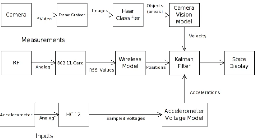
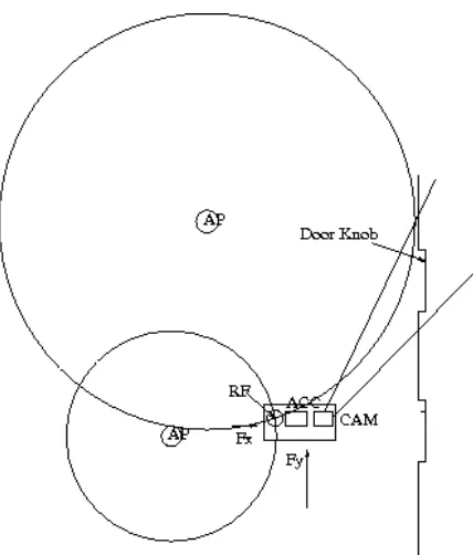
Figure 1.1: Sensor System Environmental Interaction Diagram

1.3.3

RF Sensor

The final, and perhaps most involved portion of the sensing system was the RF sensor. The

RF sensor was the only sensor used to provide directxandypositional information. The

RF sensor was a standard 802.11 card integrated into the laptop which was responsible

for the processing and integration of all the sensor data. The RF APs (accesspoints) exist

independently of the system in motion and are located at fixed positions in the external

reference frame. This means that they are, as discussed previously, absolute positioning

devices. Much research has been done on using specialized RF infrastructure [15]. In our

application we cannot use such specialized equipment. Furthermore, we are restricted to

existing infrastructure. As such only two accesspoints were available within the building

(26)

1.3.4

Overall Function

Figure 1.1 shows how the sensing system interacts with the building environment. Note

the camera looking for door locks, the RF receiving signals from two accesspoints and the

accelerometer reading the input accelerations. From this picture the above discussion of

relative versus absolute sensing should be clear. The arrows indicatingFx andFy are the

input forces felt by the cart, which are measured by the accelerometer. The circles indicate

the distance of the system from each of the accesspoints. Notice how one of the intersection

points is labeled RF, which is the RF antenna on the cart. The camera, labeled as CAM, is

identifying a door lock which is in its field of view.

At this point the general purpose and environmental interaction of each of the sensors

should be clear. Further details about the RF localization are discussed in chapter 2. Details

about visual localization are discussed in chapter 3 and details about inertial localization

are discussed in chapter 4. Chapter 5 discusses the integration of the sensor information

and chapter 6 discusses the experimental setup and results. Lastly, there is discussion of

(27)

Chapter 2

Wireless Localization

2.1

RF Techniques for Self-Localization

Given that we are trying to develop an accurate and low-cost self-localization system, with

the rise in the availability of high bandwidth wireless LAN technologies, an 802.11a/b/g

based system presents itself as the best choice for an RF localization system. As the

au-thors of [15] present, for indoor localization better than 10 meter accuracy is required.

That implies that system bandwidth must be at least 30MHz, which makes 802.11 an ideal

choice([15],1), especially with the higher bandwidth of 802.11g which allows close to 6

meter accuracy (in theory) [16]. The ideal solution would be a ultra-wide band (UWB)

technology such as wireless universal serial bus (WUSB); however, there is currently

lit-tle commercially available hardware that uses UWB technology. UWB and specifically

WUSB promises bit-rates around 480Mb/s which would allow for sub-meter accuracy at a

range of around 3-5 meters [15].

The theory behind the potential accuracy of high-bandwidth RF systems for localization

comes from the propagation time and wavelengths of RF signals. Assuming that an

electro-magnetic wave travels at the speed of light, or300,000,000m/sthen the distance that one

period of that wave propagates in a second (the wavelength) is given by equation 2.1 where

C is the speed of light,λis the wavelength andν is the frequency.

(28)

Thus, waves with a smaller wavelength yield a higher localization precision potential.

Re-arranging equation 2.1 allows equation 2.2 to show that for a precision (wavelength) of 10

meters a 30MHz signal is required [16].

c ν =

300000000m/s

30000000s−1 = 10m (2.2)

There are ways to improve that accuracy using interpolation, which are explained in

[36] as the GPS system uses several such techniques.

The method presented in [15] is a time delay of arrival (TDOA) technique. This is a

technique based on the compromise between complexity and accuracy. For this work, a

re-ceived signal strength indicator (RSSI) technique was the only one implemented; however,

a TDOA technique is also discussed because it provides a look at other RF localization

techniques ([15],2). The reasoning behind only using the RSSI technique is simple.

Com-mercial accesspoints, such as were present in the building of operation, do not have any

support for TDOA (or for that matter any) localization techniques. RSSI techniques do not

require support from the accesspoints. In keeping with the requirement to utilize existing

infrastructure no modifications were made to the accesspoints.

The TDOA technique essentially measures the delay between when a packet is sent and

when it is received. This requires the accurate synchronization of the clocks of the wireless

access-points (APs) and in this case that was accomplished with custom hardware([15],4).

In the interests of keeping the self-localization technique low-cost and within the existing

infrastructure, custom hardware for access points is unacceptable, yet the technique is still

valid. The accuracy obtained was 2.4 meters at best([15],6).

The next relevant technique was presented in the paperRadio Interferometric

Geoloca-tion[18]. The authors of [18] introduce a technique aimed to address the major issue with

TDOA based RF techniques, which is the very fast rate at which electromagnetic radiation

propagates through air. The idea they propose is:

... to utilize two transmitters to create the interference signal directly. If the

(29)

will have a low frequency envelope that can be measured by cheap and simple

hardware readily available on a WSN node. ([18],3).

Two RF signals that are close in frequency will interfere with each other and the envelope

of that interference will be of a lower frequency, thus supporting easier localization. The

reason it is easier to TDOA localize with a lower frequency signal is because the time

synchronization does not need to be as precise as with a high frequency signal. A full

discussion of TDOA and radio interferometric techniques is beyond the scope of this work.

The issue with this particular technique is that two receivers are used[18]. Our experimental

setup only has one receiver because the goal of our research is to try an find the absolute

position of a single client, not relatively localize various clients. In larger networks of

self-localizing ubiquitous computing devices this technique would be interesting because there

would be multiple receivers that could relatively locate themselves.

The chosen wireless localization technique was a simple RSSI with an interpolated and

calibrated signal strength meter.

As a basis for comparison on the differences between RSSI and GPS the following

explanation of the operation of the GPS system is presented. The reason for comparing our

system with GPS is that GPS is the de-facto standard localization system currently in use

for outdoor localization. Even though GPS receivers do not typically work indoors, they

are used in cell phones, cars, airplanes and numerous other ubiquitous devices. It is perhaps

the most successful localization system currently in use. A GPS receiver, which does not

transmit any information to the GPS satellite network, can localize itself anywhere on the

Earth within 10 meters (1 meter for military units) [36].

A GPS system works as follows [36]:

1. The basis of GPS is “triangulation” from satellites.

2. To “triangulate,” a GPS receiver measures distance using the travel time

of radio signals.

3. To measure travel time, GPS needs very accurate timing which it achieves

(30)

4. Along with distance, you need to know exactly where the satellites are in

space. High orbits and careful monitoring are the secret.

5. Finally you must correct for any delays the signal experiences as it travels

through the atmosphere.

In a simple form, GPS measures the time for a signal to arrive at a receiver by aligning a

repeating code. Transmitting a higher bandwidth code provides better accuracy.

At the beginning of this work it was estimated that sub-meter accuracy was possible.

However, several key limitations became apparent as the system was implemented. Note

that the reason for not using GPS is that GPS signals are often hard or impossible to receive

indoors.

When choosing an RF localization method the RSSI method was selected because it is

the only method available with COTS hardware which was within the existing

infrastruc-ture. TDOA techniques would have required custom hardware and firmware, as was done

(31)

Chapter 3

Computer Vision for Localization

3.1

Introduction to Computer Vision

One of the major aspects of this work has been the application of a visual sensor,

specif-ically a camera, to assist in the localization process. In order for the camera to provide

useful data it, like any other sensor, must be calibrated. Given that the nature of a camera

is different from other sensors the issue deserves some special attention.

3.1.1

Camera Model

The first step in the process of using a camera for localization, even before calibration, is

the selection of a model for the behavior of the camera. One of the most common models

is the pinhole camera model.

Pinhole Model

The pinhole camera model relies on the idea of perspective projection. That is to say a

point in the world with the coordinatesP = (x, y, z)is projected to a collinear point on the

image plane with coordinatesp= (u, v, λ). The image plane is said to be a distanceλaway

from the origin of the camera frame. This is illustrated in figure 3.1. Furthermore, the point

(32)

[image:32.612.170.450.86.293.2]

Figure 3.1: Camera Coordinate Frame([22],379)

the points are collinear, the equations describing their mapping is shown in equation 3.1.

u=λx

z, v =λ y

z (3.1)

Thus(u, v)are used as the image plane coordinates[22].

Given that an image is stored as a matrix of discrete gray levels a pixel in the image is

said to be located at(r, c), where(0,0)is considered to be the top left corner of the image.

Therefore, it is necessary to find a mapping between (u, v) and (r, c). This mapping is

given by equation 3.2, wheresxandsyare the size of a pixel and(or, oc)are the pixel array

coordinates of the principle point.

−u

sx

= (r−or), −

v sy

= (c−oc) (3.2)

A more thorough discussion of the pinhole model may be found in [22].

Other Models

While the pinhole model is perhaps the most common and most simple model, there are

(33)

[image:33.612.172.451.99.264.2]

Figure 3.2: Line Projection onto Unit Sphere([19],2)

in equation 3.3, wheremis a unit vector andf is the focal length of the camera. Note that

the projection is not defined forP = (0,0,0)T_.

P 7→m = P

||P|| =

1

p

u2₊_v2₊_f2



   

u

v

f



   

(3.3)

While this technique was not directly applied to this work it is representative of other

methods of modeling a visual sensor.

3.1.2

Camera Calibration

Once a model has been chosen the camera must be calibrated to be able to recover the world

point (x, y, z) from a given pixel value (r, c). Simply, the process of camera calibration

is the determination of the intrinsic and extrinsic properties of the camera. Examples of

intrinsic properties would be lens focal length and lens distortion. Examples of extrinsic

properties would be the pan or tilt of the camera.

Using the pinhole model as discussed above, the mapping from the 3d world

coordi-nates is given by equation 3.4, which is a combination of equations 3.1 and 3.2.

r=−λ

sx

x

z +or, c =− λ sy

y

(34)

[image:34.612.206.415.89.263.2]

Figure 3.3: Camera Distance Model

It is sufficient to know the ratios fx = _sλ_x and fy = _sλ_y. When using a typical camera

calibration approach[22] we need to find fx, fy, or, oc, which are the intrinsic parameters

of the camera and do not change with motion. However, in this work a typical camera

calibration was not used as it was not possible to determine all the extrinsic camera

param-eters (specifically distance to target). Without all the intrinsic and extrinsic paramparam-eters it is

not possible to recover the camera frame coordinate points. Additionally, we do not know

the coordinates of door lock which is in frame because all the door knobs are identical.

Therefore, uniquely translating the CP to the world coordinate frame is not possible.

3.2

System Camera Model

Due to the above presented issue with the camera system the following alternate technique

was employed. The camera used a visual model which was created from empirical data

as intrinsic data was not available. Given that the object identifier always provided square

regions, thexandyscales were treated as proportional and the area of the region was used

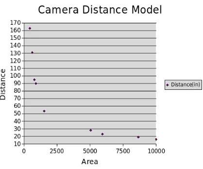
to compute the distance. A plot of the raw data used to create the camera distance model is

shown in figure 3.3. The distances are in inches and the area is in square pixels. The model

(35)

Area (in sq.) Ln Distance(m)

441 1.42

784 0.88

1521 0.31

5041 -0.34

5929 -0.54

8649 -0.73

10000 -0.9

625 1.2

[image:35.612.229.392.87.241.2]

900 0.83

Table 3.1: Camera Model Raw Data

The actual theoretical model is based on equation 3.1 which specifies projection from the

CP to the object([22],380), however this theoretical model is nonlinear and a linear model

was desired so that it could be interpollated on the fly by the imaging system as

computa-tional implementations for nonlinear interpollation are beyond the scope of this work. Do

note that the error from this approximation is bounded and decreases exponentially as is

shown in [5].

The linearized model for the aformentioned data is shown in equation 3.5 whereycam

is the estimated distance from the detected object andmcam andbcamwere calculated from

the data shown in table 3.1 by a linear least squares fit.

ycam =exp(mcamaobj+bcam) (3.5)

In this experiment the data provided mcam = −0.0002226291 andbcam = 1.075. A

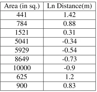
sample image where the system has detected a door lock is shown in figure 3.4. Once the

door lock detector was functioning then it was possible to obtain velocity data from the

detection subsystem. Recall that for reasons of minimizing error accumulation is was

de-sirable to minimize the integration of data, which leads to computing velocity as a natural

choice, since, for reasons previously discussed, obtaining position directly was not

possi-ble. From a theoretical standpoint equation 3.6 demonstrates where the integration errors

(36)

[image:36.612.201.419.92.277.2]

Figure 3.4: A Detected Door Lock

constant representing an error in the measurement.

x(t) +t =

Z

˙

x(t) +dt (3.6)

Given that the door locks are a constant known size (2 inches by 2 inches) it is possible

to compute the change in distance from the lock and also to track the motion of the door

lock within the frame. The goal of the system was not to be robust to orientation changes

and as such thex axis was fixed so that it was aligned with the center of the camera axis

and the y axis was perpendicular to that axis along the ground plane. The system model

particulars will be addressed further in section 5.1. Thus, changes in the size of the door

lock provided an estimate to thexvelocity while changes in the horizontal position of the

door lock in the frame provide an estimate of the y velocity. Using the aformentioned

camera model and a known door lock size of 2in sq. provided a way to compute the

correspondence between a pixel and a real distance, using a simple ratio. The computedx

andyvelocities were then available to the rest of the system. This technique is a variant of

mapless navigation where the system has

no explicit representation at all about the space in which navigation is to take

(37)

The authors of [14] feel prudent to note that all techniques rely on the fact that the vision

system must have some kind of a-priori knowledge about what they are supposed to see.

The objects of opportunity in this instance are specifically door locks.

Interestingly, it is presented that vision based localization requires the following steps([14],3):

Acquire sensory information. For vision-based navigation, this means

ac-quiring and digitizing camera images.

Detect landmarks. Usually this means extracting edges, smoothing, filtering,

and segmenting regions on the basis of differences in gray levels, color,

depth, or motion.

Establish matches between observation and expectation. In this step, the

sys-tem tries to identify the observed landmarks by searching in the database

for possible matches according to some measurement criteria.

Calculate position. Once a match (or a set of matches) is obtained, the system

needs to calculate its position as a function of the observed landmarks and

their positions in the database.

However, there are many uncertainties associated with the observations of the camera.

Therefore there needs to be a way to mitigate these uncertainties. In [33], the authors

essentially use a midpoint approximation between two samples. In [14] the authors present

Markov localization, Markov processes, Kalman filtering based on Gaussians, intervals and

deterministic triangulation as possible solutions.

Given the lack of robustness and the complexity of searching a large database of objects

to be matched, in different orientations, a different technique needs to be investigated. Viola

et al.in [37] present a technique which uses features that are similar to Haar basis functions

to classify images. A feature, as is presented, is the, “difference between the sum of the

pixels within ... rectangular regions”([37],4). This is important because the OpenCV library

(38)

In the paperVision-Based Localization Algorithm Based on Landmark Matching,

Trian-gulation, Reconstruction, and Comparison[20] David Yuen and Bruce MacDonald present

a technique for global localization. They define global localization as identifying “position

with respect to some external frame using only thecurrentsensory data” ([20],1).

Yuen and MacDonald claim that localization methods can be classified as iconic and

feature based. Iconic techniques try to match the current raw visual sensor input against

a previously acquired image set. Feature-based techniques compare prominent features

extracted from the raw image data ([20],1). An example of a feature based technique would

be extracting the room number from an image of a door sign. Similarly, matching the

whole image of the door and sign against a previously acquired image would be an iconic

technique. Feature-based techniques were applied to this work because of their simplicity,

(39)

Chapter 4

Inertial Localization

4.1

Inertial Navigation for Self-Localization

Inertial navigation, when applied to localization, provides a way of knowing, when

re-stricted to the 2-dimensional case, velocity and heading. In the three dimensional case

knowing attitude is also possible, thus allowing the determination of the pitch, roll and

yaw of the object in motion. This is possible without any external reference data through

the use of accelerometers and gyroscopes (gyros) ([35],1). This is a result of Newton’s

laws of motion, specifically that a moving body “continues to move with the same velocity

unless acted upon by an external force and that such a force will produce a proportional

acceleration of the body”([35],2). Gyroscopes are required to provide information about

the orientation of the body within the world space.

Weston and Titterton, in [35], describe the various different varieties of inertial sensing

devices. Navigational grade inertial navigation systems (INS) are far too expensive to be

practical for this work. However, cheaper, less accurate alternatives are appropriate for

this application. The background introduced below about the essential functions of INS

is applicable, although it will be modified as the research herein is restricted to the use of

accelerometers. Processing angular information (i.e.heading) is beyond the scope of this

work. Essential functions which an inertial navigation system must perform are([35],2.):

(40)

from which its attitude relative to a reference frame may be delivered.

• Measure specific force using accelerometers.

• Resolve the specific force measurements into the reference frame using

the knowledge of attitude delivered from the information provided by the

gyroscopes.

• Have access to a function representing the gravitational field – the

grav-itational attraction of the Earth in the case of systems operating in the

vicinity of the earth.

• Integrate the resolved specific force measurements to obtain estimates of

the velocity and position of the vehicle.

Herein we aim to resolve only the 2D position, without attitude compensation. Thus,

the accelerometer used will be aligned parallel with the axis of motion and used to measure

the specific (Fx,Fy) forces. Weston and Titterton note that INS is inherently prone to the

accumulation of errors and that one solution is the recalibration of the system with external

reference data ([35],12). Recall that herein we have mentioned that INS is a relative

posi-tioning system and that for the reason of error accumulation we propose to use two sources

of external location data, RF and Vision. Interestingly, after the discussion of the state of

INS presented in [35], it would appear that INS requires the use of gyroscopes. However,

a more recent paper, which will be discussed next, presents a method of determining the

attitude (as it was called) or heading from only an accelerometer-based system.

Tan and Park, in [27], present a method for determining the feasibility of using a given

physical configuration ofN accelerometers for determining both the location and

orienta-tion of an object. Note that for the purposes of this thesis we are trying to avoid unnecessary

complication (and therefore expense) of the INS and thus restricting our sensor platform

from rotational movement (only the platform, the camera may operate independently) so

this work is not directly applicable, but it is representative of what is possible using only

(41)

like device for indoor localization. These devices are commonly found on belt clips and do

not undergo rotations of a nature relevant to this work. As note, in the rotations found by

turning a corner would only change the relative X and Y axis of the accelerometer.

Han-dling inertial rotations has been well studied and hanHan-dling them was beyond the scope of

the work.

In [27] it is shown that for 3D INS based only on accelerometers, 6 accelerometers

are required. The simplest feasible configuration is to place the accelerometers in a cube

configuration which allows the state equation developed to have a closed form solution

([27],4). Unfortunately, this INS system is prone to positioning errors which grow with

time and would require recalibration to bound the error ([27],9), which is a similar problem

(42)

Chapter 5

Sensor Integration

5.1

System Modeling

5.1.1

Introduction

Any system or subsystem where the behavior needs to be classified must have a model.

Fre-quently models are developed empirically based on a simple experiment. In this work both

empirical and theoretical models were used. The overall system model was a theoretical

dynamic model in a state-space representation.

5.1.2

Experimental System Model

A state space model was chosen for the overall system as the system is a multiple input

multiple output system and state space descriptions manage that setup cleanly. The system

model is based on a simple mass with friction model in two dimensions.

The choice of the simple mass with friction model was based on the nature of the cart

on which the system was mounted. The cart had four casters with a low rolling resistance.

The dynamics of the system are given in equation 5.1. Specifically, the F_mcaptures the input

force (which is measured by the accelerometer). The _mb captures the rolling resistance of

the wheels which causes the cart to stop moving unless an input force is present. Friction

(43)

that the model describes the cart slowing down if F is0, which is the real behavior of the system. Also notice that the rolling resistance opposes the direction of motion, which is

also true of any wheeled system. Both dimensions x and yare considered as the system

may move along the ground plane.

The one dimensional dynamic equation is shown in equation 5.1, wherex¨is the overall

acceleration felt by the cart, F is the input force and b is the friction force opposing x˙,

which is the velocity.

¨

x= F

m − b

mx˙ (5.1)

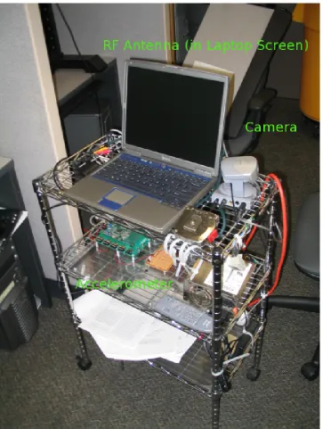
Given that herein we have a setup which is on wheels, as shown in figure 5.1, the friction

force is not a static or kinetic friction but a rolling resistance. Given that the system was on

carpet with small casters a high value for rolling resistance was chosen. A chart of rolling

resistance values is available at [39]. Thus the state input and output matrices are shown in

equations 5.2 and 5.3. Note that these are the continuous time equations.

The choice of these dynamics were dictacted by equation 5.1. The choice of b was

meant to capture the forces on the system which oppose the velocity and cause the system

to come to a stop. The two principal forces which are proportional to velocity are drag

and rolling resistance. Drag force at low velocity, such as the system was subjected to, is

negligible and was ignored. The rolling resistance caused the system to roll to a stop rather

rapidly and could not be ignored. Due to the fact that finding published values of rolling

resistance coefficients for hard casters on commercial carpet is both difficult and unreliable

the rolling resistance was estimated based on how fast the physical system cart would come

to a stop. The value ofbused was0.4905. Actual determination of rolling resistance is an

involved process and is beyond the scope of this work. Rolling resistance as well as static

(44)

[image:44.612.130.493.139.620.2]

(45)

        ˙ x ¨ x ˙ y ¨ y         =        

0 1 0 0

0 −0.4905 0 0

0 0 0 1

0 0 0 −0.4905

                x ˙ x y ˙ y         +         0 0 1 0 0 0 0 1           Fx m Fy m   (5.2)   x y  =  

1 0 0 0 0 0 1 0

          x ˙ x y ˙ y         (5.3)

The above equations are in the standard state space form shown in equations 5.4 and 5.5,

whereAc, Bc, Cc, Dcare the continuous time state matrices andxis the vector of states and

˙

xis the vector of the derivatives of the states anduis the system input vector.

˙

x=Acx+Bcu (5.4)

y=Ccx (5.5)

In order to use the model it needed to be discretized because of the sampled nature of

the measurements. The system was discretized by using a zero-order hold equivalent as

described in [25]. The reason that a zero order hold equivalent (ZOH) was chosen is that

the sensors can only provide data at the sampling times. It is desirable to have the model

respond only to the actual values of input and not a combination of current and previous

inputs, which is the role of the Kalman filter, to optimally weight current and past inputs and

states. Essentially, the system model needs to provide the Kalman filter with its response

to current inputs only and allow the filter to handle previous inputs.

As described in chapter 3 of [25] the zero-order hold is achieved by clamping the output

of the sampler at the instant that sample is available. That value is then held until another

sample is available. This technique does not impose any delay on the system but provides

poor information about the signals between sampling times, we were not concerned with

sub-sampling the information, only the data at the sampling times. This idea was driven by

(46)

[image:46.612.97.528.85.319.2]

Figure 5.2: System Block Diagram

The accelerometer provided a continuous analog signal which was sampled by a 68hc12.

The samples were taken and output at approximately 30Hz. Note although the bandwidth

of the ADC was hardware limited at 50Hz. Notice also that 30Hz is well below the Nyquist

frequency of 100Hz required for reconstruction. The goal here was not to be able to

re-construct the sampled signal, but rather use that data as acceleration information, which

means that the overall system bandwidth is more relevant. The 30Hz was chosen because

the localization system was bandwidth limited by the processing time of the vision system

and 30Hz was the maximum frame rate of the NTSC video signal. The RSSI frequency

was approximately 4Hz. This was limited by the wireless card and drivers. The driver

layer took about 250 milliseconds to collect, process and return signal strength information

to the user’s program.

Given the above discussion that data from the various sensors was sampled and that

no further delay was desired a zero order hold was the appropriate choice. Using a

zero-order hold equivalent required the computation of the matrix exponential which is a rather

(47)

the discrete time matrices are used and Matlab includes a routine to compute the matrix

exponential. The theory describing why a matrix exponential is required comes from the

solutions of differential equations. A full discussion of solutions to discrete time systems is

beyond the scope of this work and may be found in [8]. In this case it was useful to be able

to rediscretize at different sampling times for testing purposes and as such a framework to

compute the matrix exponential was implemented using Algorithm 11.3.1 from [10]. The

discrete time matrices for a sampling time of 1/20 are shown in equations 5.6 and 5.7. The

reason that Ts = 1/20was used is that was that maximum frame rate the camera could

provide. As data was only available from the sensors at a given interval those were the only

samples to consider. A faster sampling time would have created additional computational

effort without any gain because the same value (held by the zero order hold) would have

been held again.

Notice that the RSSI frequency of 4Hz is well below the sampling time. It was desirable

not to handicap the system by only sampling when all the sensors were available. It is

also impossible to ascertain exactly how fast the RSSI information would be available.

Sometimes the driver would provide that information instantly, other times it would delay.

It depended on the update packets from the APs. If the RSSI readings were unavailable it

was treated as a drop-out. Drop-out management is discussed further in section 7.2.3.

       

x(k+ 1) ˙

x(k+ 1)

y(k+ 1) ˙

y(k+ 1)

        =        

1 0.04939 0 0 0 0.9758 0 0 0 0 1 0.04939 0 0 0 0.9758

               

x(k) ˙

x(k)

y(k) ˙

y(k)

        +        

0.00124 0 0.04939 0

0 0.00124 0 0.04939

          Fx m Fy m   (5.6)  

x(k)

y(k)



=





1 0 0 0 0 0 1 0

         

x(k) ˙

x(k)

y(k) ˙

y(k)

        (5.7)

(48)

about discretization of systems may be found in [25] and [8].

x(k+ 1) =Adx(k) +Bdu(k) (5.8)

y(k) = Cdx(k) (5.9)

5.2

Kalman Filtering

Perhaps the most common technique for sensor fusion and the one which has been chosen

for this work is the Kalman filter. The discrete Kalman filter is a set of equations that define

an optimal recursive state estimator, as a solution to the linear data filtering problem([3],1).

The Kalman filter is used to combine sensor measurements corrupted by noise to obtain the

best (in a linear least squares sense) possible estimates of the system states. The Kalman

filter provides estimates of all four sensor states, however, we only concern ourselves with

xandybecause those states indicate the position of the system.

xk =Axk−1+Buk−1+wk−1 (5.10)

zk =Hxk+vk (5.11)

For a system defined by 5.10 ([3],2), whereAis the system state matrix,Bis the system

in-put matrix,wk−1is the process noise, which is assumed to have a normal distribution([3],2),

the measurement is defined by equation 5.11, wherevkis the measurement noise, which is

also assumed to have a normal distribution([3],2). These two random variables are defined

by equations 5.12 and 5.13.

p(w)∼N(0, Q) (5.12)

p(v)∼N(0, R) (5.13)

In practice, the process noise covarianceQ and the measurement noise covarianceR

ma-trices might change with each time step or measurement. The process noise covariance

(49)

equation 5.15. In this work the process noise was chosen based on the suggestions

pre-sented in [3]. This is because, as stated in [3], actual determination of the process noise can

be complicated and advanced process noise modeling is beyond the scope of this work.

Q=



      

1e−3 0 0 0 0 1e−3 0 0 0 0 1e−3 0 0 0 0 1e−3



      

(5.14)

TheRmatrix was determined by classifying the sensor error variances empirically through

trials. The data used for computing those variances is shown in appendix F.

R =



      

1.0787 0 0 0 0 0.001452 0 0 0 0 2.929 0 0 0 0 2.028



      

(5.15)

The next state estimate is defined by

ˆ

xk = ˆx−_k +Kk(zk−Hxˆ−_k) (5.16)

wherexˆ−_k is the previous known state estimate andKkis the Kalman filter gain.

The Kalman filter gainKkis given by

Kk =Pk−H

T₍_HP−

k H

T ₊_R₎−1 _(5.17)

whereP_k−is the a priori error covariance estimate andRis the measurement error covariance([3],2).

Welch and Bishop describe it in plain terms as such:

Another way of thinking about the weighting byKkis that as the measurement

error covariance R approaches zero, the actual measurement zk is “trusted”

more and more, while the predicted measurementHxˆ−_k is trusted less and less.

On the other hand, as the a priori estimate error covariance P_k− approaches

zero the actual measurement zk is trusted less and less, while the predicted

(50)

This gives an intuitive description of the Kalman filter and it’s operation.

In order to apply the KF to this work each of the sensor readings had to be provided

to the aforementioned KF framework. The accelerometer provided acceleration readings

which were used as inputs to the system, which means the values were placed into the

u(k)vector. This is shown in equation 5.18, where Fx

m is the xacceleration measurement

from the accelerometer and Fy

m is theyacceleration measurement from the accelerometer.

Note that because of the variety of notations used in the literature with the Kalman filter

equations we stateu(k)≡uk.

u(k) = uk= 

 Fx

m Fy

m 

 (5.18)

Similarly, the camera and RF measurements were provided as state measurements to thezk

vector as shown in equation 5.19, wherex˙camis thexvelocity measurement from the

cam-era,y˙camis theyvelocity measurement from the camera,xrf is thexposition measurement

from the RF system andyrf is theyposition measurement from the RF system.

zk = 

      

˙

xcam

˙

ycam

xrf

yrf 

      

(5.19)

This then defines the H matrix, shown in equation 5.20, so as to relate the camera and

accelerometer measurements to the appropriate system states.

H =



      

0 1 0 0 0 0 0 1 1 0 0 0 0 0 1 0



      

(5.20)

Recall that equation 5.2 defines thexstate as the xposition of the system, they state

(51)

The Kalman filter provides the mathematically provable best combination of the

sen-sors information. By the best combination we mean that for a given loss function (a

func-tion which penalizes incorrect estimates) the expected value of the error is minimized.

Kalman himself notes that minimizing the expected estimation error is just one possible

objective([28],37). A full discussion of the required criteria and reasoning for the choice

of that loss function is beyond the scope of this work and may be found in [28].

The minimization of the average error is very desirable. It means, in plain terms, that

the system should be providing the estimate of our position which is closest to our actual

position based on the previous and current data. However, Kalman states that in order for

the estimation error to be minimized the error must be zero mean. The key point of this

is that in order to have the optimal estimate be a linear combination of all previous

obser-vations the error processes must be Gaussian. This is so that the random variable which

minimizes the average loss (and consequently the square of the error) may be explicitly

specified[28].

The assumption that the errors present will be Gaussian in nature deserves some

atten-tion. Noise and error within physical systems is typically caused by a number of different

sources. It can be shown that a number of independant random variables summed together

can be closely approximated by a Gaussian probability curve([23],8). On a strictly practical

level it is difficult to measure statistics about the noise and error beyond mean and variance.

Therefore, there is no better assumption than Gaussianness[23].

5.2.1

Handling Data from Multiple Sensors

The next major area of research to address is the combination of the individual localization

data. Given that the entire purpose of this work is to attempt to improve upon the existing

localization techniques, it is important to discuss some of the previous localization attempts

as well as the techniques that are involved in fusing the sensor data. First some clarifications

about terminology. The terms fusion, combination and hybridization refer to, as noted in

(52)

all the different sensor data([32],1). Cooperation is a slightly different idea that typically

refers to the use of one sensor to recalibrate another once that second sensor has passed a

given error threshold, as was done in [32].

Qi and Moore, in [24], present a simplified technique to integrate GPS and INS

sens-ing. As opposed to the typical extended Kalman filter, with its associated time-variant

covariance matrices, they use a “direct” Kalman filter, which is simpler. The novel part of

this technique is that all nonlinearities are removed by preprocessing the GPS and INS data

([24],1). In this work similar preprocessing is done only with the RF data as the

accelerom-eter is guarnteed to be linear within1.25%over the whole input voltage range, although it

is typically linear within0.2% [6]. The RF is preprocessed by fitting to a quadratic curve

to eliminate some of the time-variant effects. The INS measurements are represented in

dynamic form with feedback position and velocity measurements ([24],2). The GPS

equa-tions, which in our case will be representative of the RF equations as both techniques are

similar, are algebraic in nature. Qi and Moore also state that the Kalman filter, which is

typical of such sensor fusion problems, provides state estimates of position, velocity, GPS

clock errors (in our case this would be RF signal strength errors (RSSI errors)), and drift of

the INS ([24],2). Thus they develop a model to which the standard Kalman filter model is

applied (see [24],5).

Qi and Moore state in their simulated results that, “the proposed integration method

gives better performance than the first option, GPS resetting” ([24],6). GPS resetting is a

sensor coordination technique where the GPS is used to reset the information from the INS.

They claim that the advantage to this approach, and the same reason it is attractive for this

work is:

GPS preprocessed data are taken as measurement input ... INS preprocessed

data is taken as an additional information to the state prediction... The

advan-tage of this approach is that a simple and linear Kalman filter can be

(53)

Kalman filter framework presented in [24] provided a simple way to integrate the three

(54)

Chapter 6

Experimental Setup and Results

6.1

Experiment Outline

The experiment in this work was designed with the idea that a localization system

func-tioning within a building would have an initial estimation of the system position provided

by GPS or another similar system. Alternatively, the starting position of the device might

be known by measurement from a common reference point, which would be the case with

many desirable ubiquitous systems. The iRobot Roomba1is one such system.

Any variety of localization system needs a (0,0) reference point. The zero point, or

origin as it is sometimes called, is truly arbitrary but all pieces of the system must

acknowl-edge and agree upon that point. The other issue is that all measurements and estimates

must be converted into common units of measure. For this work the SI metric system was

chosen. Any units that were in feet or inches were converted to meters before their fusion

with the rest of the system.

Once common units and an origin point have been se

Self-localization in ubiquitous computing using sensor fusion

Rochester Institute of Technology

Self-Localization in Ubiquitous Computing using Sensor

Thesis Release Permission Form

Copyright 2006 by Jeffrey Michael Domenic Zampieron

Abstract

Contents

List of Figures

List of Tables

Chapter 1

Background & Definitions

Description

Localization Focused Ubiquitous Systems

Basics of the Sensor System

Camera Sensor

Inertial Sensor

RF Sensor

Overall Function

Chapter 2

Chapter 3

Camera Model

Camera Calibration

System Camera Model

Chapter 4

Chapter 5

Experimental System Model

Kalman Filtering

Handling Data from Multiple Sensors

Chapter 6