UK house price convergence clubs and spillovers

This is a repository copy of UK house price convergence clubs and spillovers. White Rose Research Online URL for this paper:

http://eprints.whiterose.ac.uk/93073/ Version: Accepted Version

Article:

Montagnoli, A. and Nagayasu, J. (2015) UK house price convergence clubs and spillovers. Journal of Housing Economics, 30. 50 - 58. ISSN 1051-1377

https://doi.org/10.1016/j.jhe.2015.10.003

Article available under the terms of the CC-BY-NC-ND licence (https://creativecommons.org/licenses/by-nc-nd/4.0/)

eprints@whiterose.ac.uk https://eprints.whiterose.ac.uk/ Reuse

Items deposited in White Rose Research Online are protected by copyright, with all rights reserved unless indicated otherwise. They may be downloaded and/or printed for private study, or other acts as permitted by national copyright laws. The publisher or other rights holders may allow further reproduction and re-use of the full text version. This is indicated by the licence information on the White Rose Research Online record for the item.

Takedown

If you consider content in White Rose Research Online to be in breach of UK law, please notify us by

UK House Price Convergence Clubs and Spillovers

Abstract

Using a number of advanced statistical methods, this paper analyses the conver-gence and spillover effects of house price across UK regions. In contrast to the single steady-state often assumed in modern macroeconomic analyses, we find that house prices across UK regions can be grouped into four clusters, confirming the heterogeneity and complexity of the UK housing market. Moreover we document the dynamics of house price spillovers across regions.

Keywords: Regional house prices; Heterogeneity; Convergence; Spillovers.

1

Introduction

The role played by the housing market in the latest financial crash and the following

Great Recession, has led macroeconomic theory to investigate the contribution of housing

wealth to the business cycle. This is frequently discussed by incorporating into a DSGE

framework the household sector1_{, whose consumption depends upon income and housing}

wealth.2 _{The ultimate aim of the literature is to understand whether housing has an}

impact on economic fluctuations (see e.g. Iacoviello and Neri (2010)) in order to improve

the forecastability of the business cycle and to formulate appropriate policy responses.

The model solution is provided by nonlinear equations, which are then linearised (orlog

-linearised) so as to obtain fluctuations around the steady state as well as decision rules.

This is similar to the assumption that the economy is subject to only small disturbances

and, importantly, the resulting equilibrium is unique. Since the steady state is defined

under certain modelling conditions, it is important to evaluate whether this prediction

and uniqueness are supported by the data.

We contribute to the literature by testing whether the UK housing market is

charac-terized by a single long run equilibrium, which all economic regions converge to. Although

the UK housing market has been subject to extensive research, there is no clear agreement

on whether a long-run convergence path exists. Early studies (e.g. MacDonald and Taylor

(1993)) fail to find a robust convergence path; more recently Cook (2006) suggests that

the previous negative evidence might be caused by asymmetric adjustment across regions.

Holmes and Grimes (2008) find favourable evidence but suggest that moving towards a

long-run equilibrium could be slow and takes quite a long time.

To this end, the novelty of this paper consists of the implementation of a log t test

(Phillips and Sul (2007b)) to test whether multiple equilibria (i.e. convergence clubs) are

present.3 _{This approach has attractive features regarding the treatment of the steady}

state (or the common factor); among others, we can not only estimate the number of

steady states among regional markets endogenously by the data, but can also analyze the

compositions of convergence clubs. Furthermore, we complement our analysis by looking

1

The DSGE stands for the dynamic stochastic general equilibrium.

2

See Iacoviello (2010, 2011) for a review and the influential model presented in Iacoviello and Neri (2010).

3

at house price spillovers across regions, and analyse the differences in the dynamics that

drive return (i.e. inflation) and volatility spillovers over time for UK regions. The variance

decomposition analysis based on the vector autoregression (VAR) model allows us to

identify spillovers due to return and volatility shocks.

In a nutshell, our results suggest the presence of multiple steady states (convergence

clubs) in the UK housing market. While London’s housing market is very influential

over other regions’ (i.e., the ripple effect), inter-regional effects are also observed within

convergence clubs, yielding regional diversity in the UK housing market. This departs

from a single steady state often assumed by macroeconomic models.

2

Literature survey

Numerous studies have investigated the dynamics of national and regional house prices.

We can identify two strands in the literature. The first is concerned with house price

valu-ation; here, the main objective is to understand the link between economic fundamentals

and property valuation, both at a national and at a regional level (see e.g. Cameron

et al. (2006)). The aim is to try to identify which macroeconomic factors can help

policy-makers to detect possible deviation from fundamentals and the formation of bubbles. As

Muellbauer and Murphy (2008, p. 5) explain, “the deviation of prices from long-run

fun-damentals is then the bubble-burster.” More specifically, house prices may surge due to

a series of positive shocks to fundamentals such as households earnings. Thus, the

ex-pectation of further appreciation leads to overvaluation, but in due course the realisation

that improvement in fundamentals has been outpaced by house price increases, leads to

a slowdown in the rate of appreciation.4 _{McMillan and Speight (2010) analyse deviations}

of house prices from fundamental values in terms of the present value model of the asset

price literature. Here the price of an asset is explained by the fundamental, which is the

expected future payoffs of the asset itself; in the stock market literature these payoffs

are dividends, while for bonds they are represented by interest and principal payments.

The theoretical underpinning for the hypothesis that current price earnings ratios predict

4

future movements in stock prices. In applying this methodology to the housing market

the authors utilize the price-to-income ratio to investigate possible irrational deviations

from fundamentals, nevertheless we should expect the current price-to-rent ratio, rather

than price-to-income, to fit the theoretical model and predict future movements in house

prices. In fact it is the rent rather than the personal income which represents the stream

of future payoffs for the owner of the dwelling.

The second strand in the literature investigates the dynamics developing in regional

property prices and the possible existence of a ‘ripple effect’. If regions were geographically

close entities then standard economy theory would suggest that the level of house prices

within a certain area would be determined by the local demand and supply. Hence house

prices across regions would be on different levels and would move independently although

they would be still determined by similar economic factors (e.g. demographic factors

and economic conditions). This idea was first challenged by Meen (1999) who introduced

the possibility of a ‘ripple effect’ in the housing market. This refers to the fact that

changes in the housing market are first observed in one region (usually the core region),

and then they are transmitted to the adjacent regions, followed by propagation to other,

more peripheral, regions. He suggested that this effect is driven by four different factors:

migration, equity transfer, spatial arbitrage and spatial patterns.

Starting from the seminal paper by Meen (1999) the literature has proposed testing

this hypothesis using various econometric techniques. The first approach has been to

use cointegration analysis to investigate the notion of a causal long-run link between

different regional house prices, in this spirit the works of, among others, MacDonald and

Taylor (1993) and Alexander and Barrow (1994).5 _{Results for the UK economy are not}

conclusive, while MacDonald and Taylor (1993) and Alexander and Barrow (1994) find

that a long-run relationship exists, Ashworth and Parker (1997) cast doubts on these

results. A second econometric approach to test the ‘ripple effect’ is by a using unit root

test. As Cook (2005) explains, the diffusion of changes in house prices that the ‘ripple

effect’ implies, is consistent with a constant long-run ratio of regional to aggregate house

prices. He finds that the aforementioned ratio is stationary for a number of UK regions

5

thereby supporting the notion of a ‘ripple effect’.6 _{More recently, Holmes and Grimes}

(2008) find that the first principal component of the differentials between regional and

national houses prices is stationary, implying that UK regional house prices are driven by

a single common stochastic trend.

We follow more closely the second strand of the literature. In particular, we test for

multiple equilibria (i.e. convergence clubs) in the various housing markets across the UK

and then investigate spillovers across the UK.

3

Econometric framework

This paper uses mainly two statistical approaches in order to analyze regional inflation.

First, we use the logt test to examine if there is convergence in regional inflation. There

are other approaches for convergence analysis, such as the principle components approach

(e.g., Homes and Grimes (2008)) and the panel unit root tests (e.g., Levin et al. (2002);

Im et al. (2003)). But these methods are not as suitable as the log t test to analyze

con-vergence clubs because it is difficult to identify the composition of regions in concon-vergence

clubs by the former approach, while the latter does not address convergence clubs at all

since the unit root tests are a statistical method to detect a conditional convergence, in

which the steady state can differ among all regions. The log t test deals with these two

issues.

Second, data will be decomposed using the quantitative method (Diebold and Yilmaz

(2009)), in order to study spillover effects from one region to others, a method which

was originally developed to study spillovers in financial asset prices and has never been

applied to inflation analysis.

3.1

The log

t

_test

For the analysis of convergence, we shall use the Phillips-Sul method (Phillips and Sul

(2007b)); assume that panel data Xit with time (t = 1, ..., T) and country (i = 1, ..., N)

is decomposed to the permanent (ait) and transitory (git) components.

6

Xit=ait+git (1)

Since both components (ait andgit) may contain a common factor across regions (µt),

equation (1) can be re-expressed as:

Xit=

(ait+git) µt

µt=δitµt (2)

Having recovered the time-varying idiosyncratic factor δit, the common factor will be

calculated as cross-sectional average of the panels under investigation. Since Eq. (2)

suggests the presence of convergence of Xit if δit exhibits such evidence, the behaviour

of the common factor is not the main focus in our definition of convergence. In other

words, although this approach restricts to a single steady state case in a panel (Xit), the

stationarity of the steady state will not affect our analysis of convergence.

Furthermore, the idiosyncratic component (δit) is assumed to follow the following

specification which is discussed as suitable for economic data (Phillips and Sul (2007b)).

δit =δi+σiξitL(t)−1t−α (3)

Following Phillips and Sul (2007a,b), L(t) has a form of logt, and ξit ∼ IID(0,1).

Sinceδi andσi are region-specific fixed terms and given that logtis an increasing function

over time, whether or not Xit converges toward δi will be determined by the size of α.

They show that the convergence is ensured ifα ≥0, and this null hypothesis can be tested

using Eq. (4).

log(H1/Ht)−2log(L(t)) =a+blog(t) +ut (4)

where L(t) =log(t+ 1), Ht = (1/N)

PN

i=0(hit−1)2 and hit =Xit/N−1

PN

i=1Xit. Eq.

(4) suggests that, all other things being equal, a large log(H1/Ht) corresponds to a large

b. This in turn follows that Ht → 0 as t → ∞, which suggests that hit → 1 as t → ∞.

The latter implies that Xit approaches the cross-sectional average and thus is evidence of

convergence. Alternatively, a negativeb becomes evidence of non-convergence. Thus, the

convergence hypothesis is tested by the null hypothesis ofb= 0 against the alternative of

Since a rejection of the null does not necessarily imply that there is no convergence

among regions which did not form an initial convergence club. The strategy is to search

for convergence across all combinations of regions untilN−k = 1, where k is the number

of regions in convergence clubs. This terminal condition is the case where there is no

further subgroup since multiple regions are required for the study of convergence.

3.2

Spillovers

The spillovers across regions are analysed using the Diebold and Yilmaz (2009) framework.

For brevity of exposition consider a covariance stationary bivariate VARyt =A1yt−1+etor

alternativelyyt= Θ(L)etin a moving average form. This can be re-written asyt=B(L)ut

where B(L) = Θ(L)Q−1

t , ut=Qtet,E(ut, u′t) =I and Q−

1

t is the lower-triangle Cholesky

factor of the covariance matrix of et. The one-step ahead forecast (yt+1,t =Ayt) has an

error vector given by:

[

et+1,t=yt+1−yt+1,t=B0ut+1

 

b0,11 b0,12

b0,21 b0,22

 

 

u1,t+1

u2,t+1



 (5)

The variance of the one-step ahead error in forecastingy1tisb20,11+b20,12 andb20,21+b20,22

is that in forecastingy2t. Moreover, following Diebold and Yilmaz (2009) the off-diagonal

elements are the cross-market spillovers. The spillover index is then defined as:

S = b

2

0,12+b20,21

b2

0,11+b20,12+b20,21+b20,22

100 (6)

The model can easily be extended to the case of N = 12 and 4-step ahead forecasts as

in our case, and our analysis is based on VAR(1) which is determined by the Schwarz

information criterion. Furthermore, in order to obtain results robust to the order of

variables in the VAR, we implement a decomposition method, the generalized impulse

response function, which was developed by Koop et al. (1996) in the context of the

4

Data

Quarterly data on house prices for the twelve UK regions are obtained from Lloyds

Bank-ing Group. These data are classified by region; the North, York & Humberside, North

West, East Midlands, West Midlands, East Anglia, South West, South East, Greater

London (hereafter London), Wales, Scotland and Northern Ireland. The price data are

standardized and seasonally adjusted, and cover the period from 1983Q1 to 2012Q3. This

data set has been previously employed by a number of researchers (e.g. Gregoriou et al.

(2014)).

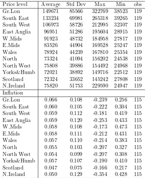
Table 1 provides a snapshot of our data set. House prices are, on average, higher in

London compared to anywhere else in the UK, for instance in Scotland, about half of

London’s price. The second part of Table 1 shows house price inflation. The inflation is

defined as the annual growth rate of house prices, i.e.,log(pt)−log(pt₋4).7 Here we do not

notice any major difference across regions; prices in London and adjacent regions tend to

grow faster but not by a large margin. Also the standard deviation does not indicate any

significant difference.

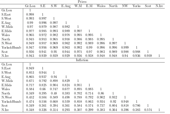
In Table 2 we provide some further evidence of the relationship among regional house

prices. Indeed, while a causality issue is not touched upon, it shows indirect evidence of

our main hypothesis of the existence of a ripple effect. In particular, both house prices and

inflation in London appear to be highly correlated with those in geographical proximity

to the region.

Furthermore, we complete our preliminary data analysis with three tests for cross

sectional dependence (Free, Pesaran, and Friedman tests). The results presented in Table

3 show that we can strongly reject the null hypothesis of no cross-sectional dependence,

implying the existence of significant spillovers in the housing market.

Overall, our preliminary analyses suggest that regional housing markets are highly

integrated to one other as their prices and inflation move in tandem with each other.

However, in the next section, more vigorous analyses will unveil some heterogeneity across

regions.

7

5

Empirical results

5.1

Multiple convergence clubs in the UK housing market

In order to apply the log t test to house prices, a matrix is created with the order of

regions based on their average house prices in the final year (i.e., 2012). Then house

price convergence will be tested by creating a subgroup which contains first the two most

expensive regions and then adding, one by one, less expensive regions to the subgroup.

Thus, Greater London (hereafter London), the most expensive region, becomes one of the

core member regions.

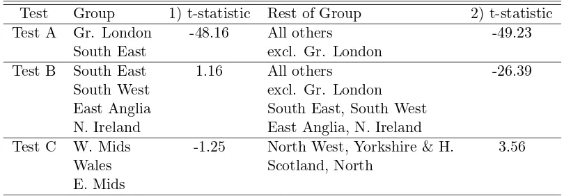
The results of the test are reported in Table 4, where we also report the estimated

t-statistics. Initially, this table shows whether London and South East (the second most

expensive region in the UK) form a convergence club, and a t-statistic of -48.16 suggests

that we can reject the convergence hypothesis. This confirms that house prices in London

are substantially different from the rest of the UK. Next, we test whether regions other

than London form a convergence club. Again no evidence of convergence is obtained with

a t-statistic of -49.23.

The next task is to check if there are any regions which exhibit convergence with

the South East. After examining all combinations of house prices in regions other than

London, we find evidence of convergence in the subgroup consisting of the South East,

South West, East Anglia and Northern Ireland. Their t-statistic is positive although it

is insignificant. Then, as before, convergence is checked among regions which have not

become a member of any convergence groups (i.e., ones excluding London, South East,

South West, East Anglia and Northern Ireland), and we find evidence of non-convergence

(t-statistic=-26.39).

In the next round, we examine if the West Midlands, the most expensive region among

the remainder, converges with some other regions. After considering all possibilities, we

find evidence of convergence among the West Midlands, Wales and East Midlands. The

t-statistic is negative but statistically insignificant, and thus the null of convergence cannot

be rejected by the data. Furthermore, the remaining regions (the North West, York &

Humberside, Scotland, and the North) are reported to form one convergence club.

clubs named Groups A to D in Table 5. Group A consists of London alone, Group B

of the South East, South West, East Anglia and Northern Ireland, Group C of the West

Midlands, Wales and East Midlands, and Group D of North West, York & Humberside,

Scotland, and the North. Interestingly the clubs seem to be spatially distributed with one

notable exception (Northern Ireland, which is not adjacent to the South East, South West,

and East Anglia). We can speculate that this anomaly is likely due to the strong price

increases in Northern Ireland in the first half of the 2000s which matches other regions in

Group B. In short, our results show evidence of heterogeneity in regional housing markets

in the UK, and it is known that regional heterogeneity in the UK housing market can

be explained by several economic factors such as migration, equity transfer, and spatial

factors (e.g., Meen (1999)).8

The presence of four convergence clubs seems to complement the previous studies

which have not found clear evidence of convergence under the assumption of a single

steady state. Our findings suggest that such a presumption itself is not supported by

the data, and they emphasize deciding an appropriate number and composition of each

convergence club prior to detailed convergence analyses; otherwise, the results would

become less credible.

5.2

Spillover effects

Panels A and B in Table 6 present the spillover effects across regions for annual house

price inflation and inflation volatility (squared inflation), respectively. The ij cell is the

estimated contribution to the forecast error variance of region i coming from innovations

to region j. Hence summing the off-diagonal terms in each row of the matrix we obtain

Contributions from Others, while Contributions to Others are obtained by adding up the

terms in the columns. So, for instance, innovation in London housing market returns are

responsible for 18.2 percent of the error variance in forecasting South East returns, but

only 5.9 percent of the error variance in forecasting Scottish returns. From Table 6 we have

two major effects; firstly, as expected, there is a higher spillover across adjacent regions.

Second, the Spillover Index is obtained by dividing the sum of the Contributions from

8

Others by the Contributions to Others including Own. This indicates that 79.6% and

73.2% of the forecast error variance of annual inflation and volatility, respectively, can be

explained by spillovers. However, this spillover effect is quantitatively more pronounced

for the peripheral regions than for the core regions, while price innovations in other

regions have limited impact on London and southern England. The result corroborates

and supports the idea of a ripple effect from London prices to other regions. Interestingly,

it should also be noted that the ripple effect from London seems to become weaker as

regions are located further away from London.

Furthermore, from this table we find that the level of self-generating inflation becomes

proportionally less important as one is distant from London, i.e., from Group A to Group

D. For return (inflation) spillovers, the importance of self-generating inflation in London

and Group B is about 26 and 30 percent respectively, and drops to around 14 percent

in Groups C and D. This proportion is high in Group B due to Northern Ireland.9 _If

we remove the effects of Northern Ireland, London is the region with the highest ratio of

self-generating inflation. This general trend remains the same for volatility spillovers and

demonstrates the dominance of London over the rest of the UK.

In addition, consistent with our preliminary analyses (Section 4), we can observe the

notable size of spillovers within convergence clubs. Indeed, about 29 to 72 percent of return

spillovers are generated in their own and neighboring regions in the same convergence

clubs. This excludes a case of London, and is calculated for example as 30.8 = 16.0 +

7.3 + 7.5 for the West Midlands. This seems to be one explanation for similarities in

neighboring regional inflation.

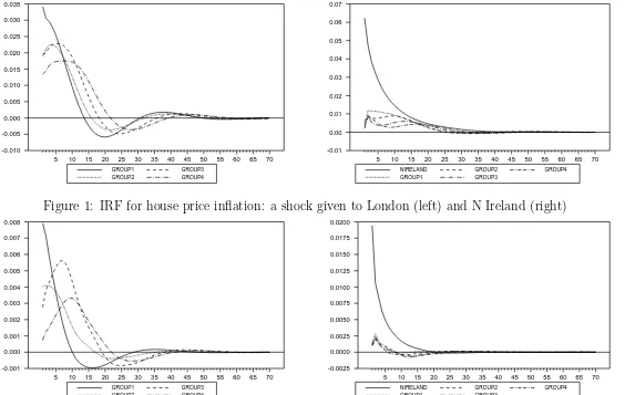
This ripple effect can also be visually presented using the impulse response functions

(IRFs). Here IRFs are again calculated by the approach proposed by Koop et al. (1996)

with a shock given to equations for price changes (Figure 1) and volatility (Figure 2) for

London or Northern Ireland for presentation purposes. The responses of other regions

to the shock are averaged out among the same club members identified in our previous

analysis. One exception is Northern Ireland which is not included in Group B in order to

differentiate regions where a shock is produced or received.

These figures show a very sharp contrast depending upon whether the shock is given

9

to London or Northern Ireland. When a positive shock is given to house price inflation

(volatility) in London, other regions follow suit. However, a shock occurring in Northern

Ireland barely affects house price inflation (volatility) in other regions. Therefore, these

figures also give rise to evidence of the ripple effect from London to other regions in the

UK, but not vice versa. Note that while the results of shocks to other regions are not

presented here, responses from such analyses are mixed and less clear than those presented

in Figures 1 and 2.

6

Conclusions

This paper looks at the convergence and spillover effects in the housing market across

twelve UK regions. We find the market to be characterized by four convergence clubs,

far more complicated characteristics in the housing market than what the conventional

macroeconomic model would suggest, and this is the first paper to quantify the number

of steady states in the UK housing market. Thus it seems vital for macroeconomists to

consider multiple equilibria in their analyses.

Moreover our results suggest the presence of a high degree of spillover across regions,

with stronger spillover effects from the core regions. At the same time, we provide evidence

of regional heterogeneity in the UK from the perspective of the housing markets, and

suggest that policymakers monitor regional economic and financial developments although

it does make sense to monitor closely London’s prices which are more likely to have useful

information to predict future housing prices in the rest of the UK through the ripple

effect. After all, even a relatively small country like the UK consists of unique regional

References

Abelson, P., R. Joyeux, G. Milunovich, and D. Chung (2005). Explaining house prices in

Australia: 1970-2003. The Economic Record 81(s1), S96–S103.

Alexander, C. and M. Barrow (1994). Seasonality and cointegration of regional house

prices in the UK. Urban Studies 31(10), 1667–1689.

Ashworth, J. and S. C. Parker (1997). Modelling regional house prices in the UK. Scottish

Journal of Political Economy 44(3), 225–246.

Black, A., P. Fraser, and M. Hoesli (2006). House prices, fundamentals and bubbles.

Journal of Business Finance & Accounting 33(9-10), 1535–1555.

Cameron, G., J. Muellbauer, and A. Murphy (2006). Was there a British house price

bubble? evidence from a regional panel. CEPR Discussion Papers 5619, C.E.P.R.

Discussion Papers.

Chen, P.-F., M.-S. Chien, and C.-C. Lee (2011). Dynamic modeling of regional house

price diffusion in Taiwan. Journal of Housing Economics 20(4), 315–332.

Cook, S. (2005). Regional house price behaviour in the UK: application of a joint testing

procedure. Physica A: Statistical Mechanics and its Applications 345(3-4), 611–621.

Cook, S. (2006). A disaggregated analysis of asymmetrical behaviour in the UK housing

market. Urban Studies 43(11), 2067–2074.

Cook, S. and C. Thomas (2003). An alternative approach to examining the ripple effect

in uk house prices. Applied Economics Letters 10(13), 849–851.

Diebold, F. and K. Yilmaz (2009). Measuring financial asset return and volatility

spillovers, with application to global equity markets. Economic Journal 119(534),

158–171.

Girouard, N., M. Kennedy, P. van den Noord, and C. Andr (2006). Recent house price

de-velopments: The role of fundamentals. OECD Economics Department Working Papers

Gregoriou, A., A. Kontonikas, and A. Montagnoli (2014). Aggregate and regional house

price to earnings ratio dynamics in the UK. Urban Studies 51(13), 339–361.

Gupta, R. and S. M. Miller (2012). The time-series properties of house prices: a case

study of the southern California market. The Journal of Real Estate Finance and

Economics 44(3), 339–361.

Holmes, M. J. and A. Grimes (2008). Is there long-run convergence among regional house

prices in the UK? Urban Studies 40(8), 1531–1544.

Iacoviello, M. (2010). Housing in DSGE models: Findings and new directions. In

O. Bandt, T. Knetsch, J. Pealosa, and F. Zollino (Eds.), Housing Markets in Europe,

pp. 3–16. Springer Berlin Heidelberg.

Iacoviello, M. (2011). Housing wealth and consumption. International Finance Discussion

Papers 1027, Board of Governors of the Federal Reserve System (U.S.).

Iacoviello, M. and S. Neri (2010, April). Housing market spillovers: Evidence from an

estimated DSGE model. American Economic Journal: Macroeconomics 2(2), 125–64.

Im, K. S., M. H. Pesaran, and Y. Shin (2003, July). Testing for unit roots in heterogeneous

panels. Journal of Econometrics 115(1), 53–74.

Koop, G., M. Pesaran, and S. M. Potter (1996). Impulse response analysis in nonlinear

multivariate models. Journal of Econometrics 74(1), 119 – 147.

Levin, A., C.-F. Lin, and C.-S. James Chu (2002, May). Unit root tests in panel data:

asymptotic and finite-sample properties. Journal of Econometrics 108(1), 1–24.

MacDonald, R. and M. P. Taylor (1993). Regional house prices in Britain: Long-run

relationships and short-run dynamics. Scottish Journal of Political Economy 40(1),

43–55.

McMillan, D. and A. Speight (2010). Bubbles in UK house prices: evidence from ESTR

models. International Review of Applied Economics 24(4), 437–452.

Meen, G. (1999). Regional house prices and the ripple effect: a new interpretation.

Muellbauer, J. and A. Murphy (2008). Housing markets and the economy: the assessment.

Oxford Review of Economic Policy 24(1), 1–33.

Phillips, P. C. and D. Sul (2007a). Some empirics on economic growth under heterogeneous

technology. Journal of Macroeconomics 29(3), 455–469.

Phillips, P. C. B. and D. Sul (2007b). Transition modeling and econometric convergence

tests. Econometrica 75(6), 1771–1855.

Phillips, P. C. B. and D. Sul (2009). Economic transition and growth. Journal of Applied

Econometrics 24(7), 1153–1185.

Stevenson, S. (2008). Modeling housing market fundamentals: Empirical evidence of

Table 1: Basic Statistics of Regional House Prices

Price level Average Std Dev Max Min obs

Gr.Lon 149671 85566 322769 38523 119

South East 133234 69981 265318 39265 119

South West 106973 58726 212995 32307 119

East Anglia 96951 51286 195604 28915 119

W.Mids 91923 48732 184958 27817 119

E.Mids 83526 44904 169528 25247 119

Wales 78924 44239 167810 25354 119

North 73324 41094 156202 24538 119

North West 75808 39886 154492 24968 119

Yorks&Humb 72021 38892 149716 22512 119

Scotland 72324 33652 145242 27808 119

N.Ireland 75820 51753 229590 24947 119

Inflation

Gr.Lon 0.066 0.108 -0.239 0.256 115

South East 0.060 0.105 -0.222 0.304 115

South West 0.059 0.112 -0.181 0.419 115

East Anglia 0.059 0.120 -0.253 0.433 115

W.Mids 0.058 0.108 -0.173 0.473 115

E.Mids 0.058 0.111 -0.212 0.431 115

Wales 0.057 0.110 -0.214 0.383 115

North 0.055 0.103 -0.207 0.327 115

North West 0.054 0.099 -0.207 0.308 115

Yorks&Humb 0.057 0.107 -0.190 0.410 115

Scotland 0.047 0.075 -0.166 0.217 115

N.Ireland 0.050 0.129 -0.354 0.428 115

Table 2: Correlation prices

Prices

Gr.Lon S.E S.W E.Ang W.M E.M Wales North NW Yorks Scot N.Ire

Gr.Lon 1

S.East 0.998 1

S.West 0.993 0.997 1

E.Ang 0.99 0.996 0.997 1

W.Mids 0.97 0.979 0.987 0.982 1

E.Mids 0.977 0.985 0.993 0.989 0.997 1

Wales 0.965 0.972 0.982 0.978 0.995 0.995 1

North 0.945 0.953 0.965 0.958 0.986 0.985 0.995 1

N.West 0.949 0.957 0.969 0.962 0.992 0.989 0.996 0.997 1

Yorks&Humb 0.947 0.956 0.969 0.963 0.992 0.99 0.996 0.996 0.999 1

Scot 0.936 0.941 0.95 0.944 0.975 0.97 0.983 0.989 0.988 0.988 1

N.Ire 0.943 0.939 0.939 0.929 0.936 0.938 0.948 0.948 0.94 0.936 0.959 1 Inflation

Gr.Lon 1

S.East 0.949 1

S.West 0.853 0.944 1

E.Ang 0.865 0.937 0.94 1

W.Mids 0.671 0.792 0.898 0.829 1

E.Mids 0.717 0.825 0.904 0.824 0.951 1

Wales 0.584 0.66 0.747 0.677 0.895 0.885 1

North 0.349 0.395 0.48 0.383 0.702 0.714 0.86 1

N.West 0.452 0.504 0.589 0.498 0.788 0.792 0.902 0.932 1

Yorks&Humb 0.474 0.556 0.668 0.559 0.858 0.863 0.934 0.92 0.948 1

Scot 0.349 0.361 0.394 0.361 0.584 0.574 0.737 0.804 0.818 0.786 1

N.Ire 0.348 0.326 0.314 0.293 0.307 0.299 0.383 0.364 0.396 0.383 0.574 1

Table 3: Cross-sectional Independence of Regional House Prices

Test type Price level Inflation

Frees 10.878 (0.000) 5.871 (0.000)

Pesaran 86.132 (0.000) 57.052 (0.000)

Friedman 1359.172 (0.000) 950.603 (0.000)

Notes:The figures in parentheses are p-values.

Table 4: The Convergence test for UK regional house price

Test Group 1) t-statistic Rest of Group 2) t-statistic

Test A Gr. London -48.16 All others -49.23

South East excl. Gr. London

Test B South East 1.16 All others -26.39

South West excl. Gr. London

East Anglia South East, South West

N. Ireland East Anglia, N. Ireland

Test C W. Mids -1.25 North West, Yorkshire & H. 3.56

Wales Scotland, North

E. Mids

Notes:The test is based on Phillips and Sul (2007b)

Table 5: The Convergence club

Clusters Regions Average price

Group A Gr. London 149671

Group B South East, South West, East Anglia, N. Ireland 103245

Group C W. Mids, Wales, E. Mids 84791

Group D North West, Yorkshire & H., Scotland, North 73369

Table 6: Spillover effects across regions

Panel A - annual regional inflation

Gr. London South-East South-West East Anglia W. Mids E. Mids Wales The North North West York.&H. Scotland N.Ireland From others

Gr. London 25.9 15.0 10.0 9.4 3.7 6.2 7.2 7.3 3.9 7.2 1.4 2.9 74.0

South East 18.2 18.1 13.5 11.7 5.8 6.5 6.3 6.9 3.7 5.6 1.7 2.0 82.0

South West 12.2 13.6 17.1 14.1 9.4 7.0 7.3 5.8 4.7 5.9 1.8 1.1 83.0

East Anglia 13.7 16.1 12.0 22.3 7.3 3.8 6.1 6.1 4.4 4.1 2.8 1.3 78.0

W. Mids 8.0 9.7 14.3 13.2 16.0 7.3 7.5 5.5 7.3 7.8 2.8 0.6 84.0

E. Mids 10.4 10.6 13.4 12.6 9.9 11.5 7.4 6.7 6.5 8.0 2.4 0.4 88.0

Wales 8.2 8.4 11.3 10.6 12.0 6.9 15.1 8.0 6.4 9.3 2.6 1.1 85.0

North 8.1 6.3 8.5 7.0 10.0 8.1 12.2 16.5 7.3 12.0 3.4 0.6 84.0

North West 7.4 6.7 11.4 7.2 10.3 8.3 10.7 8.8 13.4 12.7 1.8 1.2 87.0

York.&H. 7.4 7.5 12.2 9.1 12.2 8.8 10.0 7.7 7.3 13.8 3.2 0.7 86.0

Scotland 5.9 7.5 8.5 6.0 8.1 6.0 6.5 10.8 5.8 11.8 14.8 8.2 85.0

N.Ireland 4.0 2.6 5.6 2.8 3.3 2.1 0.7 10.2 1.3 3.6 3.1 60.7 39.0

To others 104.0 104.0 121.0 104.0 92.0 71.0 82.0 84.0 59.0 88.0 27.0 20.0 955.0

Spillover index

Including own 130.0 122.0 138.0 126.0 108.0 83.0 97.0 100.0 72.0 102.0 42.0 81.0 79.60

Panel B - regional inflation volatility

Gr. London 47.7 20.0 8.6 7.3 2.3 3.3 1.4 0.1 1.9 2.1 1.4 4.0 52.0

South East 25.6 27.7 14.7 17.1 3.0 3.3 1.1 0.7 1.4 0.3 3.1 2.1 72.0

South West 10.9 17.3 20.9 29.1 7.3 4.0 3.4 0.9 2.1 1.0 2.8 0.4 79.0

East Anglia 14.0 22.9 15.1 34.5 4.1 0.8 2.1 0.3 0.6 0.2 4.1 1.3 66.0

W. Mids 5.9 13.8 19.7 28.8 12.1 4.6 5.9 2.1 2.7 2.1 1.8 0.5 88.0

E. Mids 5.9 11.8 19.8 23.0 7.2 15.3 4.8 1.8 5.8 2.9 1.3 0.4 85.0

Wales 3.4 7.1 13.7 13.5 13.5 6.1 18.0 12.0 4.9 5.0 1.1 1.6 82.0

North 1.1 2.2 7.4 2.9 7.4 11.9 16.8 33.4 3.8 11.1 1.3 0.7 67.0

North West 3.0 5.4 12.3 7.9 9.3 10.5 16.0 11.2 12.9 9.8 0.2 1.5 87.0

York.&H. 2.9 6.9 17.1 16.4 12.9 8.7 11.4 8.5 5.1 8.2 0.4 1.5 92.0

Scotland 1.0 2.6 6.0 1.7 5.9 3.8 11.3 13.5 4.9 11.5 19.3 18.5 81.0

N. Ireland 1.9 2.3 1.4 0.2 0.9 0.3 3.1 4.0 1.4 6.6 6.3 71.6 28.0

To others 75.0 112.0 136.0 148.0 74.0 57.0 77.0 55.0 35.0 53.0 24.0 33.0 878.0

Spillover index

Including own 123.0 140.0 157.0 182.0 86.0 73.0 95.0 89.0 48.0 61.0 43.0 104.0 73.20

Notes:Variance decomposition based on Diebold and Yilmaz (2009).

GROUP1 GROUP2

GROUP3 GROUP4

5 10 15 20 25 30 35 40 45 50 55 60 65 70 -0.010 -0.005 0.000 0.005 0.010 0.015 0.020 0.025 0.030 0.035 NIRELAND GROUP1 GROUP2 GROUP3 GROUP4

5 10 15 20 25 30 35 40 45 50 55 60 65 70 -0.01 0.00 0.01 0.02 0.03 0.04 0.05 0.06 0.07

Figure 1: IRF for house price inflation: a shock given to London (left) and N Ireland (right)

GROUP1 GROUP2

GROUP3 GROUP4

5 10 15 20 25 30 35 40 45 50 55 60 65 70 -0.001 0.000 0.001 0.002 0.003 0.004 0.005 0.006 0.007 0.008 NIRELAND GROUP1 GROUP2 GROUP3 GROUP4

5 10 15 20 25 30 35 40 45 50 55 60 65 70 -0.0025 0.0000 0.0025 0.0050 0.0075 0.0100 0.0125 0.0150 0.0175 0.0200

Figure 2: IRF for price volatility: a shock given to London (left) and N Ireland (right)