Learning Relational Event Models from Video
Krishna S. R. Dubba [email protected]
Anthony G. Cohn [email protected]
David C. Hogg [email protected]
School of Computing, University of Leeds, Leeds, UK. LS2 9JT
Mehul Bhatt [email protected]
Frank Dylla [email protected]
Cognitive Systems, SFB/TR 8 Spatial Cognition University of Bremen, Bremen 28334, Germany
Abstract
Event models obtained automatically from video can be used in applications ranging from abnormal event detection to content based video retrieval. When multiple agents are involved in the events, characterizing events naturally suggests encoding interactions as relations. Learning event models from this kind of relational spatio-temporal data using relational learning techniques such as Inductive Logic Programming (ILP) hold promise, but have not been successfully applied to very large datasets which result from video data. In this paper, we present a novel frameworkremind(RelationalEventModelINDuction) for supervised relational learning of event models from large video datasets using ILP. Efficiency is achieved through thelearning from interpretations setting and using a typing system that exploits the type hierarchy of objects in a domain. The use of types also helps prevent over generalization. Furthermore, we also present a type-refining operator and prove that it is optimal. The learned models can be used for recognizing events from previously unseen videos. We also present an extension to the framework by integrating an abduction step that improves the learning performance when there is noise in the input data. The experimental results on several hours of video data from two challenging real world domains (an airport domain and a physical action verbs domain) suggest that the techniques are suitable to real world scenarios.
1. Introduction
Video is considered as a sequence of images and the area of video analysis poses several challenges. The most interesting aspect of video when compared to images is that objects (or parts of objects) in video can be perceived to move in space over time. These changes of state in the space dimension are interesting and we call them events if they satisfy certain properties such as being sufficiently frequent and having sufficiently well defined boundaries etc. An event can be a change of state of a single object, such as moving some parts of its body (for example people waving their hands) or it can be an interaction between multiple objects. Byinteractions, in this context, we mean the movement of all the objects relative to their surroundings as well as relative to each other. For example, an interaction between two objects might be both objects moving towards each other or one at rest and the other moving away from it. Before events can be recognized, we assume that the objects involved have been detected and tracked from the source video. This is not a requirement in general since some approaches (Laptev, 2005) do not require detection of objects prior to event detection.
In events involving multiple objects, interactions between the objects become a distin-guishing factor in recognizing the event instance. Capturing these interactions is the crux of event modelling and recognition as it is our hypothesis that each event can be distinguished by the interactions between the objects involved. Some events might have more than one interaction pattern that identifies the event. One way to capture these interactions is to abstract the interactions into relations between the objects. In order to represent the inter-actions of objects in an abstract form, we can use relations between the objects that depend on the spatial configuration or motion pattern of objects over a period of time. We call these spatio-temporal relations and in this paper we focus purely on the use of qualitative spatial relations since these abstract away from the metric details of particular object tra-jectories and thus facilitate the recognition of interactions as being instances of some event class (Cohn et al., 2006). There is no unique way to represent interactions using qualitative spatio-temporal relations, and the best set of relations to use depends on the domain, kind of data available (speed, orientation, size of moving objects, etc.) and the objectives of the task.
Though each event class has distinguishing interaction patterns, there are two particular challenges in event learning from examples expressed as qualitative spatio-temporal rela-tions. Firstly, automatic object detection and tracking from video is not perfect and will introduce errors into the relations. Secondly, the same event may be performed in different ways.
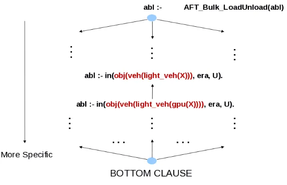
1.1 Overview of the Framework
as the extension of this procedure using abduction (explained in later sections) is applied on this relational data to obtain the event models. These event models are in the form of Prolog rules that can be used as queries in the relational data from an unseen video. From the answer substitutions we extract the spatial and temporal extensions of recognized event instances.
The main contributions1 of the paper are:
• a novel supervised relational learning framework remind for learning event models
from video and recognizing event instances using these models.
• an optimal Type Refinement operator for upward refinement of hypotheses that ex-ploits a type hierarchy in a domain for finding better event models.
• an extended framework to integrate induction and abduction in an interleaved fashion with an embedded spatial theory for improving the learning of event models.
• an evaluation of the framework on two real world video data sets (aircraft turn-arounds where the events include aircraft arrival, luggage loading and human interactions where the events are common action verbs such as exchange, follow, dig etc).
Though we concentrate on relational data obtained from tracking objects from video, the principles and techniques in this work equally apply to spatio-temporal relational data acquired from non-visual sources (e.g. laser mapping, GPS tracks, textual descriptions etc).
2. Related Work
Much of the work in event analysis (Ivanov & Bobick, 2000; Medioni, Cohen, Br´emond, Hongeng, & Nevatia, 2001; Vu, Bremond, & Thonnat, 2003; Albanese, Moscato, Picariello, Subrahmanian, & Udrea, 2007; Ryoo & Aggarwal, 2009, 2011; Morariu & Davis, 2011), does not involve learning of the models used. Instead high level event models are hand-coded using different representations (Nevatia, Hobbs, & Bolles, 2004; Hakeem, Sheikh, & Shah, 2004).
Techniques that are based on a similarity based metric in a space of low level pixel based features such as local space-time features (Laptev, 2005) are frequently used for modelling and recognizing events. These are generally more suitable for single agent events like human activities based on motion. These kind of activities generally include a particular motion signature with which an event can be recognized such as running, jumping, waving hands etc. In some event recognition systems, hand-coded high level event models are used on top of the learned low level human activity models (Ivanov & Bobick, 2000; Ryoo & Aggarwal, 2009, 2011).
One of the best performances to date in event recognition using low level pixel-based features is obtained by the Stack convolutional Independent Subspace Analysis (ScISA) (Le, Zou, Yeung, & Ng, 2011) algorithm. ScISA is based on pixel level flow based features which are then used to model events using a hierarchical representation using deep learning techniques (Bengio, 2009). The authors present an extension of Independent Subspace
Analysis to learn invariant spatio-temporal features in an unsupervised fashion instead of using predefined features.
If events are considered as a sequence of primitive states or events, state-space models are useful in representing the event models. It is also easy to hand-code the structure of the state space models, though the parameters are better if learned than encoded by hand. They provide a more robust statistical event model than hand-coded models and event recognition is done using inference on these models. Bayesian Networks are not very popular in event modelling as they lack the temporal aspect though other state space models such as Hidden Markov Models (HMM) (Rabiner, 1989) and Dynamic Bayesian Networks (DBN) (Ghahra-mani, 1998) are extensively used in event modelling and recognition. A simple HMM is not very effective in modelling complex events. Several extensions of HMM are used to suit the context and the type of event models. Hoogs and Perera (2008) proposed a DBN for jointly solving event recognition and broken tracks linking problems. The event model is a set of discrete states which expresses how the actors in the event interact over time. They assume the states are strictly ordered and this may limit learning some events that involve complex temporal relations such asduring,overlaps etc.
The main problem with state space models is that it is difficult to encode high-level temporal relations such as during, overlaps etc. The states or sub-events in an event are assumed to be in a sequential order which is not the case in many domains. Also the states are propositional in nature and hence are semantically less complex than a relational representation.
Veeraraghavan et al. (2007) learn Stochastic Context Free Grammar based models from traffic videos using predefined regions in the image. Each event model is a spatio-temporal pattern of primitive actions expressed as a string, S = a1, a2, . . . , an. The event learning algorithm aims to find a grammar that can generate the corresponding pattern for an event. The primitive actions are sequentially arranged, hence Allen’s temporal relations are not used to connect the primitive actions. Gupta et al. (2009) claim that the fixed structure of the DBNs poses serious limitations for modelling events if there are many variations in the way an event can happen. Instead they use AND-OR graphs for modelling event models. The order of the nodes imposes the causal relationship among the nodes. Because of this, some Allen relationships such as during,overlaps etc. cannot be modelled which limits its application since modelling these relations is very important in many domains.
Though low-level features and state space models are popular for simple motion patterns, it is possible to build high-level event recognition systems through several layers of reasoning. These systems use simple pattern recognition techniques to detect primitive events and then use a temporal structure to reason about complex events. The main motivation for using a high level temporal structure is that the low level features (like bag-of-features) discard most of the information regarding the relations between different entities in the data and thus makes it hard to recognize events involving complex interactions between multiple objects.
Moyle and Muggleton demonstrated using a simple blocks world that domain specific axioms can be learned from temporal observations using an ILP framework (Moyle & Mug-gleton, 1997). In work by Needham et al. (2005), the Progol system (Muggleton, 1995)
applied to the sensor data from audio and video devices. This identifies subsets of the sensor data relating to discrete concepts. Symbolic description of the continuous data is obtained by clustering within continuous feature spaces from processed sensor data. The Progol
ILP system is subsequently used to learn symbolic models of the temporal protocols present in the presence of noise and over-representation in the symbolic input data. The framework is based on time points and used only thesuccessor temporal relation.
K¨onik and Laird (2006) proposed alearning by observationframework to learn an agent program that mimics a human expert’s behaviour in domains such as games. The learned concepts are used to generate behaviour rather than classification. They applied ILP tech-niques on artificially created examples from expert behaviour traces and goal annotations. The relational data used is simple as each predicate is valid in a situation (an abstract time point) and hence concepts with sophisticated temporal relations such as Allen’s interval algebra (Allen, 1983) that use intervals cannot be learned. This limits the real world appli-cability of the framework where there are different events occurring in parallel and hence requires using Allen’s interval algebra to model them. The framework uses only positive examples and the negative examples are generated randomly in a controlled fashion.
Fern, Givan and Siskind (2002) introduced a system, leonard, that learns event
defi-nitions from videos by following a standard specific-to-general learning approach from only positive data. There are seven simple event types that are learned in this system namely pick up, put down, stack, unstack, move, assemble and disassemble. The relational data is obtained by tracking objects in indoor scenarios. No negative examples are supplied and the event models are found by computing the least-general covering formula (LGCF) of each positive example and then computing the least-general generalisation (LGG) of all these resulting formulae. When computing the LGCF of each example, the resulting LGCF will not have any interval information. Hence the model can only supportbefore andequal temporal relations between states.
The important aspect to note for the above review is that most of the work in this area has been done on either artificial or simulated data (Moyle & Muggleton, 1997; K¨onik & Laird, 2006) or very simple real world data (Fern et al., 2002; Needham et al., 2005) that involves few objects, the events are of short duration and all the objects in the scene are involved in the events. In our case, the tracked data from videos is very large and at the same time more complex and noisy and contains more objects.
pred-icates to the observation data and generalizes this data. In our case, the missing facts are because of noise in the observed data and the set of target predicates is the same as the set of observables whereas in TCIE, it is because the target predicate is not observable and the set of target predicates and the set of observables are disjoint.
Moyle (2003) introduces an ILP system (alecto) that combines abduction and
in-duction to learn theories for robot navigation. One limitation of this system is that it is restricted to positive observations only learning. The integration is not interleaved in na-ture as abduction is first used to generate explanations for each example and induction is applied on this set of explanations. This means the abduction phase does not take into consideration the concepts learned in the induction phase and dealing with noise in data was left as future work.
3. Relational Representation of Scenes in Video
To represent interactions of objects by relational data, we use spatial and temporal relations. Since the input in this work is from video, the spatial relations are defined either in the image plane or in the ground plane (if a homography is used to map the image plane to the ground plane). The spatial relations are necessary to encode the state a particular pair of objects is in. These states between two objects change as time progresses, hence we need temporal relations to connect these states. In this section, we explain how objects’ interactions are converted to relational data.
Notation: We use a first-order typed language (L) with the following alphabet: {¬,∧,∨, ∀,∃,⊃,≡,R}. LetR={r1, r2, . . . , rm}denote a set of mqualitative spatial relationships in an arbitrary qualitative spatial calculus. There are sorts (and corresponding variables) as given below (upper case letter denotes a set and lower case letter denotes a set element):
time points T — t
time intervals ∆ — δ
spatial objects O — o
events E — ε
temporal relations A— α
object types χ — τ
The special event-predicate tran(ri, ok, ol, tm)∈ E denotes a transition from a spatial relationri between objects ok and ol at time point tm. Note that in this work,α can only take values from the set of 13 Allen’s base relations (Allen, 1983) i.e. A = {before, after, meets, met by, overlaps, overlapped by, during, contains, equals, finishes, finished by, starts, started by}. We say two intervals are disjoint if the Allen relation between them is from the set {before, after, meets, met by}.
3.1 Spatial Relations
∗ →← ◦ ? ← ◦ ← ∗ ← ◦
∗ → • ? • ← ∗ •
[image:7.612.150.429.95.214.2]∗ → ◦ → ? ◦ → ← ∗◦ →
Figure 1: Qualitative Trajectory Calculus (QT CL1) (Van de Weghe et al., 2006): Each blob is a possibleQT CL1 spatial relation. In a blob, an asterix (left object) or circle (right object) represent objects in motion while a star and black dot represent objects at rest and the direction of the arrow shows the direction of motion of the object. For example, the top-left ellipse is interpreted as two objects moving towards each other and the bottom-left ellipse is interpreted as the right object is moving away from the left object while the left object is moving towards the right object (i.e the left object is chasing the right object). Though nine relations are possible in QT CL1 as shown in the figure, in practice we can reduce them to six exploiting symmetry in some relations. When only one object changes its motion state (note that an object cannot change direction without going through the rest state), the QTC relation changes along a thick line connecting two relations. When both objects change motion state instantaneously, the relation changes along a dotted line.
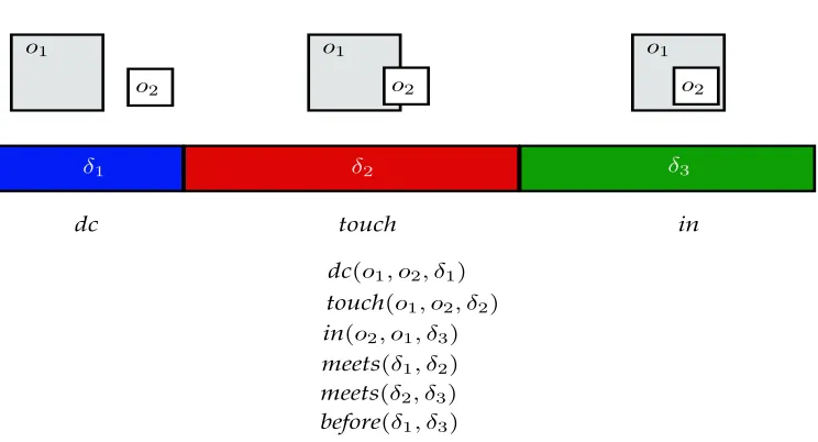
use qualitative spatial calculi to model the interactions. These interactions also have a temporal dimension as they occur over a period of time, so we extend the spatial relations with arguments modelling the temporal dimension. When we say interactions of objects we mean the interactions of the bounding boxes2 (aligned to the axes) of these objects that we get from tracking the objects using computer vision algorithms (Yilmaz, Javed, & Shah, 2006). There are different kinds of spatial calculi that target different aspects of object interactions like topology, orientation, direction, trajectories etc. and which calculi to use is a domain dependent choice (Chen, Cohn, Liu, Wang, Ouyang, & Yu, 2015). We primar-ily use three spatial relations that encode the object interactions at the topological level: dc (Discrete) when the intersection of pixels in the bounding boxes of two objects is empty, in (Inside) when the intersection of pixels is the same as the pixels in the bounding box of one of the objects and touch in every other case. This set of simple topological relations is an abstracted version3 of RCC-8 (Randell, Cui, & Cohn, 1992) spatial calculus, reduced for practical purposes without loss of essential information for event analysis. We also use
QT CL1 (Van de Weghe et al., 2006) (Fig.1) and domain specific relations as primitives to represent the interactions of objects in the videos.
2. In principle, other shape abstractions could be used as well, e.g. convex hulls, silhouettes, bounding ovals etc.
o1
o2
o1
o2
o1
o2
δ2
δ1 δ3
dc touch in
[image:8.612.121.493.97.298.2]dc(o1, o2, δ1) touch(o1, o2, δ2) in(o2, o1, δ3) meets(δ1, δ2) meets(δ2, δ3) before(δ1, δ3)
Figure 2: Converting interactions of objects to relational data.
3.2 Temporal Interval Relations
We can define temporal relations between time intervals based on Allen’s interval algebra. We usestart and end frames of an interval to represent the intervals. An advantage of this approach is, we do not have to precalculate temporal relations and store them beforehand in the database for inference. Instead, Prolog rules that calculate temporal relations givenstart andend time points of two intervals are used. In order to incorporate temporal information in describing a scenario, we extend the spatial relations with a temporal interval as an extra argument.
3.2.1 Temporally Extending a Spatial Relation
The state where a spatial relationrbetween objectso1ando2holds throughout an intervalδ is represented asr(o1, o2, δ) wherer ∈ R, o1, o2 ∈ O andδ ∈∆. Grounding this expression with objects and intervals from a database will provide us with spatio-temporal facts.
A temporal relation between two spatio-temporal facts is the Allen relation between the intervals in the spatio-temporal facts.
3.3 Representing an Event Class
An event class is represented by a set of Horn clauses where the head predicate is the same as the event name under consideration and the body is a non empty conjunction of atoms consisting of spatial and temporal predicates.
The structure of each clause in an event model for an event class εis as follows:
ε() :−β1, . . . , βi, . . . , βn
4. Deictic Supervision
For supervised learning, we need positive and preferably negative examples too of event instances. One major problem in supervised learning is collecting the labelled training data. Because of the general ambiguity in defining the spatial and in particular the temporal extent of an event (i.e. where do events precisely start and finish), it is difficult to annotate videos with event labels. A possible approach is to annotate the objects involved in each event and give the event’s temporal extent. But annotating objects is tedious and prone to human error and for some events there may be uncertainty in the objects involved. We can avoid this by usingDeictic Supervision (Dubba et al., 2010). Instead of annotating the exact objects involved in the training event instances, we only give a bounding spatial and temporal extent of each event instance which may contain other objects. The spatial extent is a region indicating where the event is happening in the video. The temporal extent is an interval which includes the actual temporal extent of the event, but may be deliberately longer in order to avoid accidentally truncating state changes relevant for the event. This makes preparation of training data easier and the learning process more robust and less biased to the labelling and the learning algorithm should be able to induce reasonable models even with this data.
Delineating spatio-temporal volumes in videos from which to learn feature-based repre-sentations of actions such as hand gestures is not without precedent in the computer vision literature (Laptev & P´erez, 2007), but our use here extends it to multiple simultaneous ac-tors and relational descriptions and resilience to perturbations in the placement of cuboids provided events are fully enclosed.
4.1 Deictic Interval and Region
In this work, a deictic spatial region is a rectangle on the image plane indicating where the event happened and the deictic interval is a time interval indicating when the event happened. A deictic spatial region is obtained by hand-delimiting the event in the image plane with a rectangle4, hence can be represented using a coordinate point (top-left corner vertex), height and width of the rectangle (x, y, h, w). A deictic temporal interval is provided by specifying the start and end time points of the interval. Together they define a space-time cuboid which delimits the spatial and temporal extension of an event.
A deictic cuboid defines a set of spatial facts and temporal relations between them; an event instance is a subset of these facts and corresponds to a positive example in the learning from interpretations setting. Obtaining positive and negative examples for learning using event annotations in the form of deictic spatial regions and deictic temporal intervals is explained in the following sections. Note that the deictic interval and region are regarded as any other interval and object in ∆ and O respectively and the spatial relations are computed accordingly. After the positive and negative examples are computed, the spatial relations involving the deictic regions as one of the objects are discarded from the database as they are of no further use.
4.2 Herbrand Interpretation for an Event
Letsi andδi be the deictic spatial region and deictic temporal interval for an instanceεi of an event classε in video v. Let Γv be the set of spatio-temporal facts present in v,Ov be the set of objects invand ∆v be the set of all time intervals in v. The set of factsEεi ⊆Γv
is the Herbrand Interpretation for the event εi over Γv iff all the facts contained in it are entailed by Γv, whose temporal intervals are not disjoint with the deictic interval and whose objects have relation touch orin within the deictic region.
Eεi ={r(o1, o2, δ) : Γv r(o1, o2, δ) ∧
Γv α(δi, δ) whereα /∈ {before,after,meets,metby} ∧
∃δ1[Γv r1(si, o1, δ1) wherer1∈ {touch,in}∧
Γv α1(δi, δ1) whereα1 ∈ {/ before,after,meets,metby}]∧
∃δ2[Γv r2(si, o2, δ2) wherer2∈ {touch,in}∧
Γv α2(δi, δ2) whereα2 ∈ {/ before,after,meets,metby}]∧
o1, o2, si ∈ Ov ∧r ∈ R ∧ δ1, δ2∈∆v
}
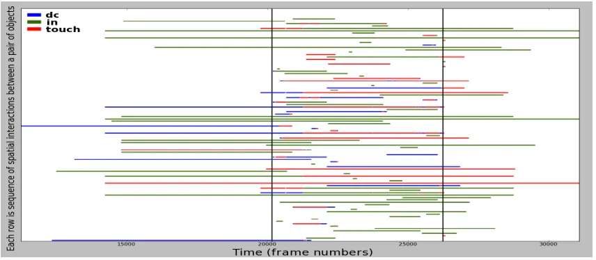
An example interpretation for an event instance ofAFT Bulk LoadUnload in the Airport domain is illustrated in Fig.3. The interpretation includes all those spatial facts involving objects that have the relation touch or in with the deictic region and which lie within the two vertical dashed lines (the deictic interval). The set of Herbrand Interpretations corresponding to the set of deictic regions and intervals for an event form the positive examples for the learning phase. The rest of the relational facts in each video form the negative example where if an event model fires an instance in the database, it is considered as a false positive. When a Herbrand Interpretation is extracted from a set of spatio-temporal facts of a video, this interpretation is independent of all the other facts in the spatio-temporal database5 for the video and hence other facts can be assumed false from this interpretation’s point of view.
Note that by definition the spatio-temporal facts that do not spatio-temporally overlap the deictic region and interval of an event instance are not relevant to the event. Considering facts outside the indicated event occurrence not only increases the size of the training data but also makes the example instances for different event classes less distinct.
One limitation of using a cuboid shaped deictic region for delineating an event instance is that it is not possible to differentiate among multiple co-occurring instances of the same event type involving different objects in a region. One way to overcome this limitation is to use more than one cuboid to enclose an event instance allowing the elimination of unwanted facts.
Figure 3: An example interpretation for the event AFT Bulk LoadUnload in the Airport domain. The vertical black lines are the start and end of the deictic interval. Each row represents the interactions of two of the objects present in the deictic region during the deictic interval in the video. The colours of the lines represent the spatial relations between the pairs of objects at that point of time. This figure does not show the effect of a deictic spatial region, but this would correspond to the elimination of certain rows (where the objects do not have a spatial relation of touch or in whilst in the deictic spatial region during the deictic temporal interval.
4.3 Herbrand Interpretation for a Non-event Interval (Negative Example)
In our framework, the negative examples are not explicitly labelled. The negative example for a given event in a video is the set of spatio-temporal facts from the database of the video that are not present in the positive examples of the event in that video. Note that the negative example will in general contain data that might be in positive examples of other event classes in that video. Another alternative is to use labelled positive examples of other events as negative examples for the event we are learning. This is convenient for classification purposes but not in recognition tasks as this will miss the background data that might be useful to minimize detections in the background regions.
Let Γεv be the union of all spatio-temporal facts from all Herbrand Interpretations of
eventεin videov. The set of facts NIεv ⊆Γv is the Herbrand Interpretation for a negative
example for event ε in video v iff it contains all the facts in Γv which are not in Γεv, i.e.,
NIεv = Γv−Γεv.
5. Typed ILP
Object
Person
Aircraft
Vehicle
Light Vehicle
GPU
Transporter
Push Back
Service Vehicle
Heavy Vehicle
Mobile Stairs
Loader
Conveyor Belt
Passenger Boarding Bridge
Container
Catering
Tanker
[image:12.612.124.490.90.340.2]Bulk Loader
Figure 4: Tree-structured object type hierarchy in the Airport domain.
many example images of objects to be detected. Even though many example images are given for training, it is not possible to capture all the possible ways an object can appear because of lighting, viewing direction, size, shape, etc. (Lowe, 2004). This may result in correctly localized objects but with the wrong categories of the objects, especially those that look visually similar in low contrast images.
When the input data is huge and noisy, there are several problems an ILP system can face. One of these is that hypothesis evaluation can take a lot of time because of the size of the data. Also the noise will tend to make the hypothesis over specific as the system learns more rules to cover the inconsistent examples. Using a typed ILP system can speed up evaluation because of typed arguments in the hypothesis (Walther, 1985; Cohn, 1989) and also reduce the number of false positives through avoiding certain cases where the types of the arguments do not match. Any event model that has objects with a specialized type will fail to recognize some event instances where the object appears with a different type. In contrast, if the event model does not have any type system and uses a very generic type for all the objects such asobject,thing etc., then this approach will have many false positives as it cannot differentiate between events with same structure but involving different types of objects. One possible approach is to find an appropriate type generalization instead of using one of the two extremes: most generic type and most specialized type.
In most ILP systems, the type hierarchy of objects is not integrated into the learning process. For example, in Progol, types of the objects are used only in mode declarations
s1
s2
s3
s4
[image:13.612.205.410.93.147.2]s5
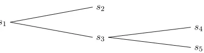
Figure 5: Tree-structured example object type hierarchy. s1 is the most general type and
s2, s4, s5 are the most specific types.
type τ2, then Progol generates two rules, one with τ1 and another with τ2. Even if we are not dealing with a vision system that introduces noise into the high level learning and reasoning system, in some cases an event might involve objects from a particular sub-group of objects. In this case, instead of using a very generic type like object or very particular types like the type of the object itself, it is more efficient to use an intermediate generic type that represents this sub-group. A variable without type restrictions will be satisfied by any type of object when instantiating the Horn clause. However, an appropriate generalization can be enforced by the learning system with a variable of typeτ1tτ2from the type hierarchy, which is satisfied6 only by objects of typeτ
1 orτ2, thereby reducing false positives.
5.1 Representing a Typed Hierarchy
If we wish to use an existing Prolog engine for hypothesis evaluation then some way of encoding type using terms must be found. There are several ways of doing this depending on whether the structure of the object type hierarchy is a tree or a lattice. We use the type representation proposed by Bundy, Byrd and Mellish (1985) that can deal with tree structured type hierarchies; we then develop a refinement operator by incorporating this representation in the hypothesis search procedure. An advantage of using this representation is that ordinary unification can be used to determine whether two types are compatible.
We will write τi < τj, if τi is a subtype of τj and τi 6= τj. Every object oof type τn in a hypothesis can be represented by the term τ1(τ2(. . . τn(o). . .)) where τ1, . . . , τn is the maximal sequence of types such thatτn < . . . < τ2 < τ1. We denote this representation function by Υ. Note that we need a constraint, i.e. a tree structured type hierarchy, in order to guarantee the uniqueness of the sequenceτ1, . . . , τn.
For example, let s1, s2, s3, s4, s5 be types such that s4 < s3 < s1, s5 < s3 < s1 and
s2<s1 as shown in Fig.5. Then any objectoof type s4 can be represented as follows: Υ(o) =s1(s3(s4(o)))
An object oi is not compatible with an objectoj in a hypothesis if Υ(oi) is not unifiable with Υ(oj). For example: s1(s3(o1)) will not unify with s1(s2(o2)) but will unify with
s1(s3(s4(o3))) and s1(s3(s5(o4))), hence they are compatible.
5.1.1 Example of Representing a Type Hierarchy
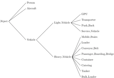
An object type hierarchy that occurs in one of the two domains used in the evaluation section of this work is shown in Fig.4. The hierarchy from Fig.4 is hand defined based
on observed errors in object classification of the tracking data from the Airport domain. In the airport domain, the ground power unit (GPU), transporter and push back vehicle are small vehicles that look similar as the videos from CCTV cameras in the airport have low resolution contrast without much colour or sharp edges. This makes it challenging to train an object detector and use it for detecting objects in these videos. The objects from the Verbs domain present no particular challenges from an automatic classification point of view but some events involve objects from a particular subset of objects, for example, thethrow event involves balls of different types likesmall ball, basket ball,etc. Hence using a type hierarchy based on utility is expected to help find event models that have better performance in detecting events in unseen videos.
A vehicle V of type GPU will be represented as obj(veh(light veh(gpu(V))))7 while V of type light veh is represented as obj(veh(light veh(V))). Note that obj(veh(light veh(V))) unifies with vehicles of type GPU and vehicles of type Trans-porter. So using obj(veh(light veh(V))) in a model can cover examples that either involve a GPU or a Transporter and hence can handle the noise from an object detector if it confuses these vehicles by outputting GPU in place of Transporter or vice versa.
5.2 Type Refinement Operator
A refinement operator is used to traverse through the hypothesis lattice. There are two types of refinement operators: upward and downward (Nienhuys-Cheng & De Wolf, 1997). We write Hg Hs if Hg is a more generic8 hypothesis than Hs. If we assume that the top most element of the hypothesis lattice is the most generic hypothesis and the bottom most hypothesis is the most specific hypothesis, then theupward refinement operator can be defined as follows (the downward refinement operator can be defined in a similar fashion):
Let L be the set of all possible hypotheses. An (upward) refinement operatorρis defined such that for a hypothesis H, ρ produces only generalizations of H, ρ(H) = {Hg | Hg
H, Hg ∈ L}.
We define the (upward) Type Refinement operator ρt as an operator that generalizes the object types ofH. Apart from object types, the structure of H and members of ρt(H) is identical.
We define a type generalizing operator as follows:
generalize type(τ1(τ2(. . . τn−1(τn(o)). . .))) =τ1(τ2(. . . τn−1(o). . .))
The Type Refinement operator, ρt, applies the generalize type operator to a selected object type present in a hypothesis, resulting in a more generic hypothesis by moving up exactly one level in the type hierarchy.
Though the specific current representation of type hierarchy using functors requires a tree structured hierarchy, having a tree structured hierarchy is beneficial from a computa-tional viewpoint in limiting the type generalizations, i.e., there are no multiple ancestors. A tree-like type hierarchy is very natural in many domains though some domains might not
7. Note the short forms used for Object, Vehicle and Light Vehicle.
have a well defined tree-like object type hierarchy. In such cases, a lattice structured type hierarchy is more suitable though this will increase the size of the search space since the number of possible refinements is increased, in particular in a tree structure type general-ization is deterministic whilst this is not the case in a lattice structure.
5.2.1 Optimality of the Type Refinement Operator
Refinement operators can be ideal or optimal (Nienhuys-Cheng & De Wolf, 1997)9. An optimal refinement operator generates any hypothesis in the hypothesis lattice only once and there is a unique way to produce each hypothesis. This kind of refinement operator is desirable in complete search algorithms as duplicate generation of hypotheses will increase the cost of the search procedure. Theoptimality of theType Refinement operator is proved in Appendix A.
6. Learning from Interpretations Setting for Learning Event Models
The result of deictic supervision gives us examples that are sets of spatio-temporal facts. Though these examples (sets of facts) come from the same or different videos, they are independent of each other, i.e., the mapping of each example to a class is independent of other examples. For this kind of learning setting where each example is independent of each other and each example is a set of facts, the learning from interpretations setting is an apt choice (Blockeel, De Raedt, Jacobs, & Demoen, 1999). The setting can be specified formally thus:
Given:
• a set of classes C (each class labelc is a nullary predicate).
• a set of classified examplesE (each element of E is of the form (Ei, c) with Ei a set of facts andc a class label)
• and a background theory B,
Find: a hypothesisH (a set of Horn clauses), such that for all (Ei, c)∈E:
• H∧Ei∧B c, and
• ∀c0 ∈C− {c}:H∧Ei∧B2c0
In the current event learning problem, the above setting is applied for each event class where in each case the set of classes has only two elements, the event class and the back-ground class. Backback-ground class represents the negative examples and each class labelcis a nullary predicate.
6.1 Traversing the Search Space
The search process for a hypothesis starts with an initial hypothesis which has a nullary predicate as head and an empty body. The hypothesis lattice is traversed using the Progol
and Type Refinement operators in an interleaved fashion. The Progolrefinement operator
is a specialization operator that adds atoms from the bottom clause to a hypothesis. A specialization operator moves from the top (empty clause) to bottom in the hypothesis space which is a lattice bounded by the bottom clause from the bottom. Adding atoms from the bottom clause makes the hypothesis more specialized because the body of the hypothesis is a conjunction of atoms and each atom can be considered as a constraint. Adding more atoms to the body increases the constraints it has to satisfy to become true.
The Progol refinement operator that we use here is based on the bottom clause also
called themost-specific clause and is non-redundant though it is not weakly-complete with respect to the general subsumption order (Tamaddoni-Nezhad & Muggleton, 2009). The most-specific clausethat the Progolrefinement operator uses can be computed from
train-ing examples, mode declarations and the background knowledge (Muggleton, 1995). Mode declarations are user defined syntactic biases in the form of predicates that specify what predicates from the background knowledge are expected in the target hypothesis and also the nature of the variables (input, output, or constant). The selection of atoms to be added to the hypothesis from bottom clause is done in a controlled manner. The atoms are only considered starting from left and moving to the right and each atom can be added only once (Tamaddoni-Nezhad & Muggleton, 2009). These constraints on the selection of atoms makes the refinement process non-redundant, i.e., a hypothesis is not generated twice. There is an additional refinement operator that refines by unifying two variables arbitrarily selected from the hypothesis or by substituting a variable with a constant. We do not use this operator as unifying two variables needs checking the hypothesis for consistency with respect to the underlying spatial theory and there are no fixed constants (apart from frame numbers) in the domain as constants in any example are independent from constants from other examples. For example, consider the three relations from Section 4.1 for the spatial theory and Allen’s relations for the temporal relations: we cannot unify two arguments of a predicate (spatial or temporal) as this violates the semantics of these relations.
Figure 6: Type refinement operator (generalization).
6.2 Searching the Event Model
Once themost-specific clauseis computed, the sub-lattice bounded from below by the most-specific clause is searched using a best-first search for the hypothesis that has a maximum score calculated based on a combination of (1) the number of positive examples covered, (2) the number of answer substitutions in the negative examples, (3) the length of hypothesis and (4) the number of distinct variables in the hypothesis subject to the given constraints (discussed in the next subsection).
score(H) =γ∗p−(%∗n+l+v) where
γ = weight to positive examples
p= number of positive examples covered
%= weight to answer substitutions in negative examples
n= number of answer substitutions in negative examples
l= length of the hypothesis
v = number of distinct variables in the hypothesis
Ananswer substitution θfor an exampleeis a substitution that grounds the hypothesis,
instead of classifying videos, a hypothesis with fewer false positives is desirable. Hence hypotheses are penalized using the number of answer substitutions10in negative examples. If the number of positive and negative examples are disproportionate in numbers, giving more weight to the positive examples and negative examples usingγ and%will result in an hypothesis that has better performance in test data.
Since the starting hypothesis is empty and completely generic, it will cover all the negative examples. As the hypothesis is specialized by Progol’s refinement operator, the
number of false positives decreases. When the score of the hypothesis no longer increases, the Type Refinement operator is used to generalize the types thereby increasing the generality of the hypothesis with a possible increase of positive examples covered (as well as false positives). This process of interleaved application of both operators is continued until the hypothesis score no longer increases.
Once a satisfactory hypothesis is found, an argument representing temporal information in the form of a list of time intervals formed using the time intervals in the body of the event model can be introduced into the head in order to explicitly representwhen the event occurs – this is useful when using the hypothesis for event monitoring – it allows the interval during which the event occurs to be explicitly flagged when viewing the video.
The learning algorithm uses a set covering method (Quinlan, 1990) to learn an event model that is a set of clauses interpreted as a disjunction. The covering method starts with an empty model and learns a clause using the provided positive and negative examples and adds this clause to the model. It repeats this procedure but now with positive examples that are not covered by the earlier clause. This process is repeated until all the positive examples are covered.
6.3 Constraining the Search Space
The size of the search space depends on the size of the bottom clause (Muggleton, 1995). Thus, in the event learning domain, it depends on the number of spatial relations being used and the number of objects in the event instances used as positive examples. The size of thebottom clauseincreases with the number of Allen’s temporal relations as each interval in the atoms with spatial predicates is temporally connected to every other interval in other atoms with spatial predicates. This creates many atoms with temporal predicates in the bottom clause.
In order to decrease the size of the search space, the algorithm makes use of domain-dependent and domain-indomain-dependent constraints on the structure of the hypothesis. The constraints the algorithm uses such as restrictions on the hypothesis length and the number of variables in the hypothesis etc. are domain-independent structural constraints as they do not depend on the predicates used or any domain knowledge. The following are the two domain-dependent constraints that reduce the search space and time thereby making the learning process more efficient.
• Upper bounds on the number of atoms in the body of a rule.
• Any interval in an atom with spatial (temporal) predicate should appear in an atom with a temporal (spatial) predicate. Any hypothesis with atoms that do not satisfy this criteria is not semantically meaningful since it might be satisfied by facts not at all related to the event in question.
However the constraints listed above are domain dependent constraints rather than ap-plication specific constraints, i.e., these constraints that involve the spatial and temporal predicates should be applicable in most, if not all event learning scenarios. Note that some of the constraints are hard (i.e. inviolate). If a hypothesis violates any such constraint, then it is discarded without scoring or refining. For example, the domain-independent constraints and the first domain-dependent constraint mentioned above are hard. In contrast, if a hy-pothesis violates a constraint that is not hard, for example, the second domain-dependent constraint listed above, it is not scored and discarded only after generating refined hypothe-ses from it. This is because discarding such hypothehypothe-ses without refining might obstruct the traversal of the lattice. For example, in the current work, the algorithm starts the search process with an empty hypothesis and the initial hypotheses obtained by refining the empty hypothesis do violate the second domain-dependent constraint listed above (since they con-tain exactly one predicate and therefore cannot concon-tain both a spatial and a temporal predicate).
6.4 Event Recognition
The learned event models are used for event recognition in unseen videos. For this purpose, the test video is converted to relational data and used as a database and the event models are used as Prolog queries. The querying is done in the whole database and the intervals extracted from the answer substitutions from these queries give the temporal extent of the recognized instances of the events. In order to record when the event takes place, we change the arity of the event predicate (the rule head) to be monadic such that the argument is a list of all interval variables occurring in the body. Note that it would also be possible to introduce a second argument to record which objects are involved in the event (i.e. a list of all variables of type object - or equivalently that occur as the first two arguments of any spatial predicate in the body).
An issue that arises is exactly when an event occurs given that it consists of multiple overlapping temporal intervals from the instantiated predicates in any given answer substi-tution. Given the list of all intervalsλoccurring in the instantiated body of the hypothesis, various possibilities present themselves. One could take the maximal interval which exactly spans all intervals inλ. Or one could take the interval which exactly spans the interval from the first transition (i.e. pair of meeting intervals involving the same pair of objects) to the last such transition. Clearly there are other possibilities too. Ultimately this is probably a domain dependent decision. For our experiments, we take the list of all intervals inλ and the temporal extension of the event is obtained by taking the minimum and maximum of the time points in λ.
7. Interleaved Induction and Abduction (IIA)
In the previous section we showed how ILP can be applied to learn rule-based relational event/activity models, given an observation dataset, positive and negative examples of events whose models have to be learnt. However, data from visual and other sensors tend to be noisy with high variability in the sample space. This leads toover-fitted models (i.e., more rules), as the model has to cover some of the examples that are corrupt because of the sensor noise. A model with more rules can result in many false positives when used for event-recognition in test data.
In this section, we show how well-fitted, semantically meaningful event models can be learned from noisy data by interleaving induction and abduction. This acquires significance in cases where training data is scarce and noisy. We apply the Typed ILP system presented in the previous section to learn event-based models and using these models as the domain theory, we explain the examples/observations not covered by the induced theory using abduction. The uncovered examples are either noisy, or are examples for the same event that in reality happened in a different way. Using the explanation we rectify the errors in the noisy examples corrupted by tracking errors and thus reduce the requirement for additional rules. In our framework, the examples themselves are noisy (i.e. incorrect) thereby requiring observation data revision in a manner that is consistent with the initially learned theory, and general common-sense knowledge aboutspace,spatial change, and the dynamics of the domain. Note that many ILP approaches discard examples considering them as noisy by using a heuristic stopping criteria. This is not acceptable in cases where there is scarcity of training data, where learning from every example is potentially important.
7.1 Domain-Independent Spatial Theory
In order to pursue our goal, an Axiomatic Characterisation of the Spatial Theory is neces-sary. Many spatial calculi exist, each corresponding to a different aspect of space. Here, it suffices to focus on one spatial domain, e.g., topology, with a corresponding mereotopologi-cal axiomatization by way of the binary relationships of the RCC-8 fragmentRrcc8. From an axiomatic viewpoint, a spatial calculus defined onR has some general properties (P1–P5), which can be assumed to be known apriori. To realize a domain-independent spatial theory that can be used for reasoning (e.g., spatio-temporal abduction) across dynamic domains, it is necessary to formalize a domain-independent spatial theory (Σspace) which preserves the high-level axiomatic semantics of these generic properties. For reasons of space we only sketch the properties P1–P5 and neglect the formal axiomatization.
(P1–P2)The Basic Calculus Properties (Σcp) describe the jointly exhaustive & pair-wise disjoint (JEPD) property, i.e., for any two entities in O, one and only one spatial relationship fromR holds in a given situation. The jointly exhaustive property of n=|R|
base relations can be axiomatized by nordinary state constraints and, similarly, the pair-wise disjointproperty can be axiomatized by [n(n−1)/2)] constraints. Other miscellaneous properties such as symmetry and asymmetry can be expressed in the same manner.
(P3) The primitive relationships inRhave a continuity structure, referred to as its Con-ceptual Neighbourhood (Σcn)(CND) (Freksa, 1991), which determines the direct, con-tinuous changes in the quality space (e.g., by deformation and/or translational motion).
on the derivation of a set of Composition Theorems (Σct) between the JEPD set R. In general, for a calculus consisting of n JEPD relationships, [n × n] compositions are precomputed. Each of these composition theorems is equivalent to an ordinary state con-straint, which every n-clique spatial situation description should satisfy.
(P5)Additionally, Axioms of Interaction (Σai) are necessary when more than one spa-tial calculus is modelled in a non-integrated manner (i.e., with independent composition theorems). These axioms explicitly characterize the relative entailments between inter-dependent aspects of space, e.g., topology and size.
Now, letΣspace ≡def [Σcp ∪ Σcn ∪ Σct ∪ Σai] denote a domain-independent spatial theory that is based on the axiomatizations encompassing (P1–P5).
7.2 Physically Plausible Scenarios
Corresponding to each spatial situation (e.g., within a hypothetical situation space), there exists a situation description that characterizes the spatial state of the system. It is neces-sary that the spatial component of such a state be a ‘complete specification’, possibly with disjunctive information. For k spatial calculi being modelled, the initial situation descrip-tion involvingmdomain objects requires a complete n-clique specification with[m(m −1)/2] spatial relationships for each calculus. Therefore, we need to define a scene description to be C-Consistent, i.e., compositionally consistent, if the n-clique state or spatial situation description corresponding to the situation satisfies all the composition constraints of every spatial domain (e.g., topology, orientation, size) being modelled. If more than one calculus is modelled the inter-dependent constraints (P5) must hold as well.
From the viewpoint of model elimination of narrative descriptions during an (abductive) explanation process, C-Consistency of scenario descriptions is a key (contributing) factor determining the commonsensical notion of the physically realizability of the (abduced) sce-nario completions. Bhatt and Loke (2008) show that a standard completion semantics with causal minimization in the presence of frame assumptions and ramification constraints pre-serves this notion of C-Consistency for Σspace within a logic programming framework, as well as with arbitrary basic action theories.
7.3 The Inductive-Abductive Framework
We interleave inductive and abductive commonsense reasoning about space, events and change within a logic programming framework. Induction is used as a means to learn event models by generalizing from sensory data, whereas abductive reasoning is used for noisy data correction byscenario and narrative completion, thereby improving the learning.
7.3.1 Explanation by Abduction
typi-cally available as sensoryobservationsfrom the real execution of a system or process. Given narratives, the objective is often to assimilate/explain them with respect to an underlying process model.
The abductive explanation problem can be stated as follows (Kakas, Kowalski, & Toni, 1992):
Given: Theory T and observationsG, find an explanation4such that:
• TS 4G
• TS4is consistent
i.e., the observation follows logically and non trivially from the theory extended given the explanation. Abductive explanations are usually restricted to ground literals with pred-icates that are undefined in theory, namely the abducibles. Abductive explanations are derived by trying to prove the observation from the initial theory alone: whenever a lit-eral is encountered for which there is no clause to resolve with, the litlit-eral is added to the explanation.
The abduction procedure results in many valid explanations. In order to reduce the number of explanations, several restrictions as listed below can be used (Kakas et al., 1992):
Explanations should be basic This means one explanation should not explain another explanation. This is enforced by not allowing abducibles in the head of any rule.
Explanations should be minimal This means one explanation should not subsume an-other explanation.
Explanations should satisfy all integrity constraints With this restriction, we ob-tain explanations that are valid in the domain under consideration. In our work, explanations should satisfy all the spatial constraints of the underlying spatial theory.
7.3.2 Scenario and Narrative Completion
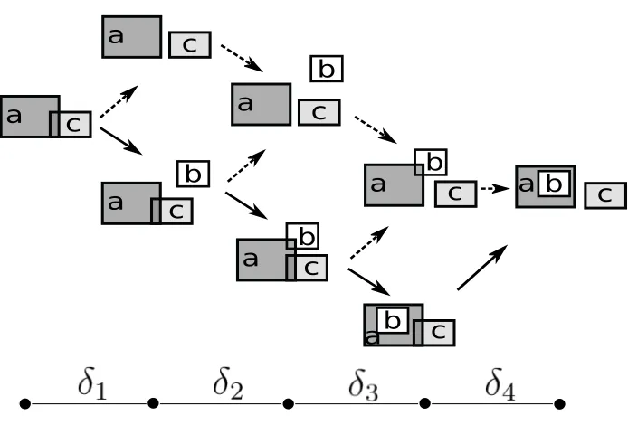
It is easy to intuitively infer the general structure of narrative completion by abductive explanation. Consider the illustration in Fig.7 for a hypothetical situation space that char-acterizes the complete evolution of a system. In Fig.7 the situation-based history given by the solid arrows represents one path, corresponding to an actual time-line discretized into intervalshδ0, δ1, . . . , δmi, within the overall branching-tree structured situation space. Given incomplete narrative descriptions, e.g., corresponding to only some ordered intervals in terms of high-level spatial (e.g., topological, orientation) and occurrence information, the objective of explanation is to derive one or more paths from the branching situation space, that could best-fit the available narrative information. Formally:
Φ1 ≡ touch(a, c, δ1)
Φ2 ≡ dc(a, c, δ4) ∧ in(b, a, δ4) ∧ dc(b, c, δ4) [Σspace ∧ Φ1 ∧ Ω] |= Φ2, where
Ω ≡ (∃δi, δj).[meets(δ1, δi) ∧ bef ore(δi, δ4) ∧ dc(b, a, δi)
∧ touch(a, c, δi) ∧ dc(b, c, δi)]
∧ [meets(δi, δj) ∧ meets(δj, δ4) ∧ touch(b, a, δj)
∧ touch(a, c, δj) ∧ dc(b, c, δj)]
a
c
a
c
a
c
b
a
c
b
a
b
c
a
b
c
a
b
c
[image:23.612.133.480.110.345.2]a
b
c
Figure 7: Branching/Hypothetical Situation Space. Only a few possibilities are shown. There are clearly more paths from the initial scenario to the target scenario. There are also more possible states.
In (7.1), Φ1denotes the initial situation and Φ2 denotes the final situation represented in terms of spatial relations (RCC-5) among the objects present in the scene. The abductive derivation of Ω, that explains how the scene changed from situation Φ1 to situation Φ2, primarily involves non-monotonic reasoning in the form of minimizing change, in addition to making the default assumptions about inertia, and an appropriate treatment of ramification constraints (Bhatt & Loke, 2008).
7.4 IIA Algorithm
The main assumption we make here is that the noise in the examples is not consistent. If the noise is consistent (i.e., present in most of the examples in a similar fashion) then it becomes part of the pattern that defines the concept and might be learned by the learning algorithm.
The pseudo algorithm is given in Algorithm 1. The induction algorithm induces an initial hypothesis based on the score function explained in previous sections. The positive examples covered (ERule+ ) by this hypothesis are removed from the list of positive examples yet to be covered. The induced theory along with background knowledge is used to explain the uncovered examples treating each example as a narrative. Abduction gives several possible explanations each with different cost (based on the nature and the number of facts in the explanation). The explanations are rejected if they have a cost more than a specified threshold. Furthermore, given the formulation of the spatial theoryΣspace,C-Consistency of abduced explanations is ensured. The examples (E4+) that have an explanation whose cost is less than the specified threshold are removed from the positive examples list that are yet to be covered, as they are now considered to be covered by the already induced model. This process of induction and abduction is repeated until all the positive examples are covered. Apart from the constraints enforced by the spatial theory to filter abduced explanations, several heuristics can be used to give a score to each explanation so that a low cost consistent explanation can be selected by the system. One of the several possible heuristics is to prefer explanations where the number of transitions in spatial relations is minimal (Hazarika & Cohn, 2002). This heuristic is a direct consequence of McCarthy’s Common Sense Law of Inertia (McCarthy, 1986) which states that change is abnormal and persistence is to be preferred in the absence of data. In a spatio-temporal domain, each explanation abduced in the absence of data is a set of spatio-temporal facts and there are three ways to add them to the explanation: (i) Extend the current relation between two objects (can be done in both directions of the timeline if the situation permits) (ii) change the current relation between two objects to its neighbouring relation in a CND (iii) introduce a new object (hypothetical) into the scene and its spatial relations with other objects in the scene as well. The cost of each explanation is based on the type of spatio-temporal fact chosen and is calculated as explained below.
7.4.1 Cost of an Abduced Explanation
Let4be an explanation from the abduction procedure where4is a set of grounded spatio-temporal facts of the formr(oi, oj, δk) denoted asfijrk,Ep+ is the current positive example (an interpretation, i.e., a set of facts) and let r be from the set of spatial relations Rin a spatial calculus. Let Obe the set of objects inE+
p. Letcfijrk be the cost of abducing fijrk.
The total cost of4denoted as C4 is X
fijrk∈4 cfijrk.
The cost of abducing fijrk is calculated as follows:
cfl =
ι, if there exists afijrm inEp+ such that δk and δm aredisjoint
κ, if there exists afijsm inEp+ such thatδk and δm are disjointand r6=s
µ∗n, wherenis the number of hypothetical objects (objects not in O) in fijrk
The first case in the cost function occurs when the system abduces a fact that extends a relation between two objects in the temporal dimension. This does not count as a spatial transition and hence has a very low cost. In contrast, the second case occurs when the system abduces a fact that extends the existence of two objects in temporal dimension with a different relation (the new spatial relation must be a neighbour to the existing relation in the CND) than the one that already exists between them. This counts as a spatial transition and has a cost more than the first case. The third case occurs if it is necessary to have a hypothetical object to satisfy the hypothesis in E+
p . This case is used when an object involved in an event is completely missed by the object tracker while first two cases are used in scenarios where an object is not detected in some temporal slice in its life time. Note that the first case is clearly the most preferred if the abduction procedure has to find a low cost explanation and the third case which is the most expensive applies when an object is completely missed by the object tracker. Though it is possible to avoid transitions to reduce the score, sometimes it is mandatory to consider transitions. For example, consider a scenario where two objects have adcrelation and in the final state they have anin relation. In this case, the algorithm has to abduce facts where there are two transitions (one when thedc relation changes totouch and another whentouch changes toin relation). Note that it is not necessary to abduce temporal relational facts as the Prolog definitions for temporal relations in the background theory can be used to compute them when needed. This can be achieved by not including temporal predicates in the list ofabducibles.
The abduction procedure uses the existing constants in the database and one issue with this is that though the number of relations and objects is small, the number of possible intervals is very large if not constrained. In order to constrain the possible explanations, we introduce intervals with predefined duration into the database so that abduction uses only these intervals for abducing explanations. Note that abduction as we have defined it only adds missing spatio-temporal information and cannot be used to retract corrupted data resulting from noise.
Algorithm 1 Interleaved Induction and Abduction algorithm (IIA)
procedure IIA(E+, E−, B) .training sets and background knowledge (includes spatial
theory)
H← ∅ 4 ← ∅
whileE+6=∅ do
Rule←Induce(B, E+, E−)
H ←HS
{Rule} E+ ←E+−E+
Rule
4 ←Abduce(B, H, E+)
E+ ←E+−E+
4 end while
return H . Learned theory
Figure 8: Airport domain: The videos are recorded using 6 static cameras looking at the same scene from different angles.
8. Experimental Results
In this section, we present an evaluation of remind, as well as the extension presented in
Section 7. For the experiments, we used two real world video datasets that are different from each other in many aspects. The videos from these datasets are shot in outdoor settings and in different weather and light conditions (rainy, cloudy, sunny, night). These variations in the videos present various challenges to the vision system and subsequently to the learning system both in the training phase and the event recognition phase.
The two datasets used in this work for evaluation are from airport logistics and verb videos. The datasets from these domains differ in many aspects such as number of objects in the video, length of video, duration of events, background structures, the number of cameras used to capture the events and also the plane (image plane or ground plane) in which the tracking data is made available. We view the differences in the datasets as a positive aspect - the framework shown to work in two very different kinds of scenarios.
remind11 is implemented in Python and for speed, some modules are implemented
in Cython; SWI-Prolog is used as the underlying Prolog engine for storing and querying relational facts and background knowledge.
8.1 Airport Logistics
For experiments in the airport logistics domain, 15 turn-arounds12 were used where each turn-around was shot using 6 cameras from different angles (Fig.8) and each video is on average one hour long (15 frames per sec).
The following are informal descriptions of the International Air Transport Associa-tion (IATA) events we aim to learn models for:
Aircraft Arrival Aircraft comes into the apron
Aircraft Departure Aircraft moves away from its position on the apron GPU Positioning Ground power unit comes and positions in its zone Left Refuelling Fuel truck arrives on the left side of aircraft for refuelling PB Positioning Push-back vehicle positioning in front of the aircraft PBB Positioning Passenger Boarding Bridge attaches itself to the aircraft PBB Removing Passenger Boarding Bridge detaches itself from the aircraft FWD CN LoadUnload Container Loading/Unloading at the front end of the aircraft AFT CN LoadUnload Container Loading/Unloading at the rear end of the aircraft AFT Bulk LoadUnload Baggage Loading/Unloading at the rear end of the aircraft FWD Bulk LoadUnload Catering Loading/Unloading at the front end of the aircraft
Within each event, there is high variability because of noise in tracking and also because of objects extraneous to the event entering the event scene. Note that some events might not be present or may occur multiple times in some turn-arounds. The scenes involve interactions of vehicles and people with zones on the apron. These zones are specified on the ground plane according to the IATA specifications and the position of the zones depends on the type of aircraft. These zones are used for parking and steering vehicles for different operations carried out in a turn-around. Note that these zones are static throughout the video and do not change size or position, unlike the bounding boxes of the vehicles obtained through tracking. Hence zones are not included in the type hierarchy used for the domain (Fig.4) since they do not suffer from visual noise. The main reason to use zones is that the RCC-5 spatial relations between bounding boxes of vehicles and people in the ground plane rarely touch, hence most of the interactions are encoded as dc if zones are not used. It is important to use the zones as most of these interactions happen in the zones. According to the IATA specifications, a vehicle transition through the zones and the position of the vehicle in particular zones is important to determine the events.
We use the object tracks provided by a partner in the Co-Friend project (Ferryman, Borg, Thirde, Fusier, Valentin, Bremond, Thonnat, Aguilera, & Kampel, 2005); certain details in some events are not detectable with this tracking system such as the direction of baggage on the rail of the loader vehicle and whether the trolleys are empty when they arrive at the scene. The Load/Unload events obtained from IATA events differ in such details (if the trolleys are loaded when they arrive at the scene and the baggage is moving towards the aircraft, then the event isloading and if the trolleys are empty when they arrive at the scene and the baggage is moving away from the aircraft, the event isunloading). Apart from these details, they are semantically similar and hence are regarded as the same events (for example, FWD CN Load and FWD CN Unload are regarded as the same events and named FWD CN LoadUnload, the same strategy is followed with other Load/Unload events).
8.1.1 Tracking and Obtaining Relational Data
single camera and because of the size of the aircraft it is possible to have many occluded objects in the scene. In order to solve these problems, six cameras are used to shoot the scene from different angles so that the entire area is covered and the number of occluded objects is minimized. Working on the ground plane data results in learned models that are independent of the camera view and the airport as these models can be readily applied at different airports with different camera configurations.
The tracking data is obtained for each of the videos from six cameras of a turn-around and fused together to get 3D data on the ground plane (Ferryman et al., 2005). The tracking data is noisy because of low quality, bad light and weather conditions and low contrast of CCTV videos. The noise can be the presence of phantom objects, missing objects, wrong types of vehicles, inaccurate bounding boxes, broken trajectories, object identity, inconsistencies etc. which are typical problems in any computer vision tracking system. Each turn-around is separately processed to get relational data that consists of a set of spatial relations among the vehicles and zones on the apron. Prolog rules that decide the temporal relationships among intervals are considered as background information in the ILP system. The data for each video has between 250 and 500 spatial relational facts (excluding temporal relational facts) depending on the number of objects and the interactions between these objects.
Note that an event requires at least one change in the state (here, spatio-temporal relations between pairs of objects) of the objects. If the relation between any two objects is dc and does not change during the life span of the objects, it signifies that the objects are not interacting and the relational fact is discarded as these spatio-temporal facts do not contain relevant information in defining event models. The tracking data also consists of bounding boxes for people in the scenes, but these are discarded as people are not germane in the semantics of the events and also these increase the size of the relational data.
8.1.2 Annotation of Events
For supervised learning we need positive and preferably negative example instances of events. In the airport domain, the temporal extent of the events is provided by indi-viduals who have expertise in the IATA protocols and apron activities, by specifying the start and end frame numbers of the event instance in that video. The spatial extent was obtained by using a tool with which a polygon can be drawn on one of the image planes and the corresponding ground plane region is obtained using an homography (it was easier for a human annotator to watch an actual video to provide the spatial annotation rather than view a 3D visualization in the ground plane, which being the fusion of the imperfectly tracked data that does not always show all relevant objects). This region gives a spatial extent for the event instance.
8.2 Physical Action Verbs Dataset
TheAction Verbs dataset13 is a corpus of video vignettes (Fig.9) that portray motion verbs such as approach, exchange, jump, collide,etc. enacted in natural environments like parks,