Void Fraction Measurement of Gas-Liquid Two-Phase Flow from Differential Pressure

This is a repository copy of

Void Fraction Measurement of Gas-Liquid Two-Phase Flow

from Differential Pressure

.

White Rose Research Online URL for this paper:

http://eprints.whiterose.ac.uk/81730/

Version: Accepted Version

Article:

Jia, J, Babatunde, A and Wang, M (2015) Void Fraction Measurement of Gas-Liquid

Two-Phase Flow from Differential Pressure. Flow Measurement and Instrumentation, 41.

75 - 80. ISSN 0955-5986

https://doi.org/10.1016/j.flowmeasinst.2014.10.010

© 2015, Elsevier. Licensed under the Creative Commons

Attribution-NonCommercial-NoDerivatives 4.0 International

http://creativecommons.org/licenses/by-nc-nd/4.0/

[email protected]

Reuse

Unless indicated otherwise, fulltext items are protected by copyright with all rights reserved. The copyright exception in section 29 of the Copyright, Designs and Patents Act 1988 allows the making of a single copy solely for the purpose of non-commercial research or private study within the limits of fair dealing. The publisher or other rights-holder may allow further reproduction and re-use of this version - refer to the White Rose Research Online record for this item. Where records identify the publisher as the copyright holder, users can verify any specific terms of use on the publisher’s website.

Takedown

If you consider content in White Rose Research Online to be in breach of UK law, please notify us by

Void Fraction Measurement of Gas-Liquid Two-Phase Flow

from Differential Pressure

Jiabin Jia

, Akintayo Babatunde

and Mi Wang

a_{School of Chemical and Process Engineering, University of Leeds, LS2 9JT, UK} b_{School of Engineering, University of Edinburgh, Edinburgh, EH9 3JL , UK}

[email protected], [email protected], [email protected]

Abstract: Void fraction is an important process variable for the volume and mass computation required for transportation of

gas-liquid mixture in pipelines, storage in tanks, metering and custody transfer. Inaccurate measurement would introduce errors in product measurement with potentials for loss of revenue. Accurate measurement is often constrained by invasive and expensive online measurement techniques. This work focuses on the use of cost effective and non-invasive pressure sensors to calculate the gas void fraction of gas-liquid flow. The differential pressure readings from the vertical upward bubbly and slug air-water flow are substituted into classical mathematical models based on energy conservation to derive the void fraction. Electrical Resistance Tomography (ERT) and Wire-mesh Sensor (WMS) are used as benchmark to validate the void fraction obtained from the differential pressure. Consequently the model is able to produce reasonable agreement with ERT and WMS on the void fraction measurement. The effect of the wall friction on the mathematical models is also investigated and discussed. It is concluded the

friction loss cannot be neglected, particularly when gas void fraction is less than 0.2.

Keywords: Differential pressure, void fraction, frictional pressure loss

1. INTRODUCTION

Two-phase flow is any type of flow containing more than one phase of liquid, gas or solid. These processes are frequently encountered in the process industries. Mean volumetric void fraction is a key parameter to characterise two-phase flows. Many researches were carried out to correlate differential pressure and void fraction in two-phase flow, but hindered by inability to generate one model that was valid for all flow regimes. This is due to the complex nature of the different flow patterns and energy interactions in flow [1]. Lockhart and Martinelli [2] gave the general correlation of pressure drop for two-phase flow. Wallis [3] fitted an equation to the plot of liquid hold up “1- g”

Electrical Resistance Tomography (ERT) and Wire-mesh Sensor (WMS) are tomographic modalities and they have more complicated measurement mechanism than pressure sensors. Both ERT and WMS can measure gas void fraction without the consideration of friction loss in the two-phase flow, which provides an alternative approach to validate the gas void fraction model based on differential pressure. The void fraction measurement accuracy of ERT and WMS were discussed by Faraj [10] and Sharaf [11]. The principle behind ERT is to determine the electrical conductivity by measuring the voltage between the ERT electrodes mounted on the internal circumference of the conveying conduit. The measured conductivity is subjected to the Maxwell’s equation [12] to calculate the local cross-sectional void fraction of the dispersed phase. This is an invasive but non-intrusive local void fraction measurement technique in two-phase mixtures, which is also capable of providing tomographic cross-sectional images. WMS consists of two planes of wire electrodes arranged perpendicularly to each other at an angle of 90 degrees covering the flowing cross-sectional area. One plane of the wires is the current transmitter while the other plane is the current receiver. The conductivity is measured by injecting a voltage pulse into one of the transmitting wires, while the other transmitting wires are kept at ground voltage [13], the current flowing to all receiving wires are measured simultaneously and conductivity estimate made from that. The void fraction of gas is derived from the normalised conductivity. Both ERT and WMS can present local cross-sectional void fraction. All local void fractions are averaged to obtain the mean void fraction.

2.

EXPERIMENT SETUP AND PROCEDURES

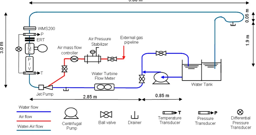
The experiment was carried out on the flow loop facility at the University of Leeds. The sketch of the flow loop is shown in Figure 1. In the experiment, air and tap water are gas and liquid phase respectively. The channel in blue represents the water flow and the red channel represents the air supply. The cyan section represents the mixed air-water flow. The stabilised air flow rate is regulated by the air mass flow controller. After the loop bend, the upwards air-water mixture goes through the flow instrumentations, 5.80 m horizontal section and then back to the water tank, where air is released and water is recycled. The detailed information on flow meters was described in literature [12].

Figure 1. Experimental flow loop

Table 1. Inlet flow rates of air and water

Bubble flow Slug flow

Water flow rate

(m3/s)

Air flow rate

(m3/s)

Water flow rate

(m3/s)

Air flow rate

(m3/s)

2.04×10-3 8.33×10-5 _9.32×10-4

5.00×10-4

1.45×10-3 _1.67×10-4

6.72×10-4 5.83×10-4

8.02×10-4 _2.50×10-4

4.11×10-4 6.67×10-4

3.33×10-4 7.50×10-4

4.17×10-4 8.33×10-4

9.17×10-4

1.00×10-3

1.08×10-3

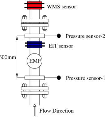
A wet/wet differential pressure sensor with two tubes was adopted first. It was not suitable for the air-water flow measurement, because the small air bubbles entering the tube affected the accuracy of readings. The diaphragm gauge pressure sensor was tested later. It worked well when the pressure inside the loop was larger than that of atmosphere, however, because of the working principle of the gauge pressure sensor, it failed to provide the correct readings if the pressure inside the loop was less than atmospheric pressure. Eventually two absolute pressure sensors (Omega PXM209) with 0~2.50 bar measurement range and 0.25% full scale accuracy were selected. The differential pressure is obtained from the subtraction of two individual absolute pressure sensors. The front-end interface of the pressure sensor is intrusive but non-invasive with fluids. The schematic of the experimental sensors is shown in Figure 2 below. Wire-mesh sensor, ERT sensor and electromagnetic flowmeter (EMF) are installed along the vertical Perspex pipe with 500 mm inner diameter. Two absolute pressure sensors are 600mm apart.

Figure 2. Installation of flow meters

Before dynamic experiment, the pressure sensors were calibrated against atmospheric pressure and static water head to eliminate the systemic error. After each water flow had been established steadily in the flow loop, reference measurement concurrently was taken for ERT and WMS. The pressure readings were sampled via a data acquisition system with 16 bits resolution of analogue to digital conversion. Upon completion of measurement taken for reference, the flow rate of water was kept constant while air was introduced at different flow rates controlled via the gas mass flow rate controller. Once the air flow rate was stable, ERT, WMS and pressure readings were taken concurrently for 10 seconds to get the mean value. The experiment procedures were repeated for different flow conditions.

Pressure sensor-2

Pressure sensor-1 600mm

Flow Direction EIT sensor WMS sensor

While the above process was running, readings were also taken for water flow rate via the turbine flow meter, air flow rate via the mass flow meter and water velocity via the electromagnetic flow meter (EMF). The fluid temperature was monitored throughout the whole process. Once all the data had been downloaded, numerical correlations shown in the next section were conducted on the data to estimate the air volumetric void fraction.

3. DIFFERENTIAL PRESSURE CORRELATION FOR VOID FRACTION

The correlation of differential pressure and void fraction is based on the classical Bernoulli’s principle of energy conservation within a flowing conduit, which states that as shown in equation (1), the sum of all forms of mechanical energy in a steady fluid along a pipeline is the same at all points.

_v2_ghP

2

1 ₍₁₎

where ½ v2 is kinetic energy, gh is potential energy and Pis pressure.

If considering the two tapping points where the pressure sensors are located, equation (1) can be developed as equation (2). p m m m

mv  gh P  v  gh2P2F 2 2 1 1 2 1 2 1 2

1_{    (2)}

where m is gas-liquid mixture density, Fp is frictional pressure loss. Since the pipe is of uniform cross-sectional

area. It is assumed force due to velocity of fluid is constant, v1= v2= v, therefore, the kinetic energy on both sides are

cancelled.

p m

mgh1P1 gh2P2F

 (3)

The tapping point of the pressure sensor 1 is regarded as reference point with the height h1= 0 and the height of

pressure sensor 2 is h2= h. Equation (3) above is simplified to

p mgh P F

P₁



Therefore differential pressure P between tapping point 1 and 2 is

p mgh F P

P

P   

 1 2



In gas-liquid two-phase flow, the mixture density m is defined from gas density g and liquid density l.

_m(1_g)_l_g_g (6)

Substituting equation (6) into equation (5) gives

P[(1









Solving for void fraction g from the equation (7) gives

gh F gh P l g p l g ) (       

 (8)

The frictional pressure loss Fp is defined as

D hv C

F_p f m

2

2 

 (9)

Before Fp is computed, the actual liquid velocity v and the Fanning friction factor Cf have to be predetermined. Cf is formulated into different format in terms of the different flow conditions and the roughness of the pipe wall.

The material of the pipe is Perspex, which has relatively smooth wall. In out experiment, the Reynolds numbers (Re= vD/µ) of all flow conditions are in the range of 3,000~100,000, therefor Fanning friction factor Cf is

simplified as the form in equation (10).

0.25

Re 079 . 0   f

C (10)

For simplicity, water dynamic viscosity µ is taken in Reynolds number. Air density g is approximated to 0

because it is nearly 1000 times less than water density l and the mass flow rate of water much is larger than the

mass flow rate of air, which caused 0.12% error of void fraction by this approximation.

Due to the complex nature of the gas-liquid two-phase flow, the on-line acquisition of the actual liquid velocity v and viscosity µ remain a challenge, which hampers the accuracy of Fanning friction factor Cf obtained. In our

study, the liquid velocity v is approximated from the division of the commingled flow rate reading on the electromagnetic flow meter (EMF) and the internal cross-sectional area of the EMF port. This velocity is an indication of the actual liquid velocity and not the superficial velocity based on the principle of operation of the EMF meter. Fluids temperature is monitored to calibrate water viscosity and density for calculating the Reynolds number. Applying these assumptions and substituting equation (9) into equation (8), void fraction g is expressed as

gD v C gh P f l g 2 2 1  

 

 (11)

4. RESULTS AND DISCUSSION

4.1. Void Fraction from Differential Pressure

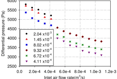
Figure 3 indicates the relationship between air/water flow rate and differential pressure. The different colour symbols represent different inlet water flow rate. When inlet water flow rate is kept constant, differential pressure decreases with the increase of inlet air flow rate. When inlet air flow rate remains constant, differential pressure decreases with the decrease of inlet water flow rate.

Inlet air flow rate(m3/s)

0.0 2.0e-4 4.0e-4 6.0e-4 8.0e-4 1.0e-3 1.2e-3

Diff erential press ure ( Pa) 2500 3000 3500 4000 4500 5000 5500 6000

2.04 x10-3 1.45 x10-3

8.02 x10-4 9.32 x10-4

6.72 x10-4

4.11 x10-4

Figure 3. Variation of differential pressure with air/water flow rate

(Inlet water flow rates are presented with different legend)

Inlet air flow rate(m3/s)

0.0 2.0e-4 4.0e-4 6.0e-4 8.0e-4 1.0e-3 1.2e-3

Air

void fr

action

0.0 0.1 0.2 0.3 0.4 0.5

2.04 x10-3 1.45 x10-3 8.02 x10-4

9.32 x10-4 6.72 x10-4

4.11 x10-4

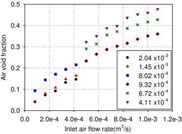
Figure 4. Variation of air void fraction with air/water flow rate

4.2. Comparison with ERT and WMS

To ensure the precision of the ERT and WMS air void fraction measurement on air-water flow, four flow conditions were configured. The experiment was repeated five times. The mean air void fraction and corresponding standard deviation of each flow condition is listed in Table 2. Data in Table 2 is exhibited in Figure 5 to show the standard deviation in the form of error bar. It is shown that the precision of ERT and WMS is on the same scale and it is difficult to conclude the superiority of two tomographic modalities. However it is noticed that ERT has smaller measurement variation than WMS when air void fraction is less than 0.05.

Table 2. Precision of ERT and WMS air void fraction measurement

Water flow rate

(m3/s)

Air flow rate

(m3/s)

Mean air void fraction from

ERT

Standard deviation

Mean air void fraction from

WMS

Standard deviation

2.04×10-3 _8.33×10-5

3.948×10-2 1.066×10-3 4.145×10-2 5.951×10-3

2.04×10-3 8.33×10-4 _2.105×1012 _9.312×10-3 _2.266×10-1 _3.504×10-3

9.32×10-4 8.33×10-5 _7.2535×10-2

8.303×10-3 6.724×10-2 8.608×10-3

9.32×10-4 8.33×10-5 _2.9707×10-1

3.148×10-3 3.043×10-1 7.017×10-3

Air void fraction from WMS

0.00 0.05 0.10 0.15 0.20 0.25 0.30 0.35

Ai

r voi

d

fractio

n

from ER

T

0.00 0.05 0.10 0.15 0.20 0.25 0.30 0.35

Figure 5. Precision of ERT and WMS air void fraction measurement

gas superficial velocity and vice versa. This is because, in the bubble flow regime, the void fraction is less due to the large volume of water that comingles with the air in this regime, this causes more drag on the dispersed gas bubbles preventing them to move through the continuous liquid phase thereby reducing the void fraction, but a change in trend is seen in the slug flow regime when the gas superficial velocity is increased given the air bubbles more energy in moving up through the continuous water phase without the drag noticed in the bubble flow regime.

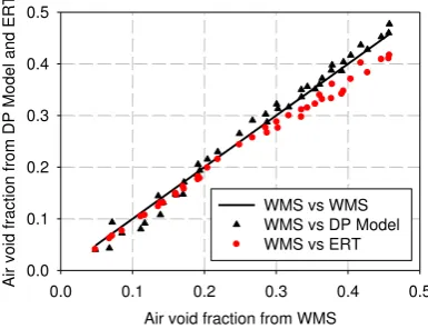
Comparison between ERT and WMS has been discussed in pervious literature [12]. ERT and WMS have good agreement when air void fraction is less than 0.25. However, it is apparently noticed that the void fraction from ERT is underestimated when void fraction is more than 0.25. Void fraction from DP model has great match with WMS void fraction estimations, particularly if void fraction is larger than 0.2. It is also noticed that void fraction from DP model has larger discrepancy with that from WMS when air void fraction is less than 0.2. The reason might because at these flow conditions, the absolute pressure readings belong to the lower range of pressure sensor’s full measurement range, although differential pressure between two pressure sensors is larger (5000~6000 Pa in Figure 3). A standard differential pressure sensor should overcome this problem. The term of frictional pressure loss in equation (8) plays an important role towards calculating void fraction less than 0.2. Section 4.3 focuses on the discussion on this issue.

Air void fraction from WMS

0.0 0.1 0.2 0.3 0.4 0.5

Air

void fr

action f

rom

DP M

odel

and ERT

0.0 0.1 0.2 0.3 0.4 0.5

WMS vs WMS WMS vs DP Model WMS vs ERT

Figure 6. Air void fraction comparison for WMS, ERT and DP Model

4.3. Impact of Frictional Pressure Loss on Void Fraction Estimation

Air void fraction

0.0 0.1 0.2 0.3 0.4 0.5

R

e

la

tiv

e

d

iffe

re

n

ce

(%

)

0 10 20 30 40 50 60 70

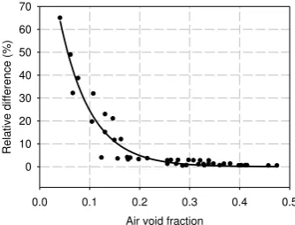
Figure 7. Relative difference with and without pipe wall friction

5. CONCLUSIONS

Two absolute pressure sensors are used to measure differential pressure. The method has benefits of low capital cost and ease of installation, however, the accuracy of pressure measurement might not be sufficient at the lower range of sensor’s full scale. The differential pressure model based on energy conservation is re-derived based on a few assumptions. Experimental results show that the void fractions obtained from differential pressure model has good agreement with those obtained from Electrical Resistance Tomography and Wire-mesh sensor. Results also show that the term of pipe wall friction in differential pressure model has larger effect on the air-water flow with smaller air void fraction. This term cannot be neglected when air void fraction is smaller than 0.2. When air void fraction is larger than 0.2, the relative difference of void fraction caused by neglecting pipe wall friction is less than 3%. In summary these findings will help in the estimation of void fraction for multiphase flow systems, which will serve as a platform for further engineering studies in the area of multiphase flow metering.

REFERENCES

1. Á. G. Német, "Maximum Liquid Transport. Flow of Gas-Liquid Mixtures in Vertical Tubes", Industrial & Engineering Chemistry, 53, 1961, pp. 151-154.

2. R. W. Lockhart and R. C. Martinelli, "Proposed Correlation of Data for Isothermal Two-Phase, Two component Flow in Pipes". Chemical Engineering Process, 45, 1949, pp. 39-49.

3. G. B. Wallis, One Dimensional Two Phase Flow, USA, McGraw-Hill Book Company, 1969.

4. J. C. Merchuk and Y. Stein, "Local Hold-up and Liquid Velocity in Air-lift Reactors". AIChE Journal, 27, 1981, pp. 377-388. 5. C. Tang and T. J. Heindel, "Estimating Gas Holdup via Pressure Difference Measurements in a Cocurrent Bubble Column".

International Journal of Multiphase Flow, 32, 2006, pp. 850-863.

6. A. H. Hasan, "Multiphase Flow Rate Measurement Using a Novel Conductance Venturi Meter: Experimental and Theoretical Studi in Different Flow Regimes". Ph.D. Thesis, University of Huddersfield, 2010.

7. A. Sharquet, I. Ismail and M. N. Karsiti, "Study of Void Fraction Measurement in a Two Phase Flow by Using Differential Pressure and Electrical Capacitance Tomography". Mathematical/Analytical Modelling and Computer Simulation (AMS), Fourth Asia International Conference on, 26-28 May 2010, pp. 408-413.

8. H. Müller-Steinhagen and K. Heck, "A Simple Friction Pressure Drop Correlation for Two-phase Flow in Pipes". Chemical Engineering and Processing: Process Intensification, 20, 1986, pp.297-308.

9. S. D. Gharat and J. B. Joshi, "Transport Phenomena in Bubble Colunm Reactor II: Pressure Drop", The Chemical Engineering Journal, 48, 1992, pp. 153-166.

10. Y. Faraj, M. Wang, J. Jia, Q. Wang, C. Xie, G. Oddie, K. Primrose and C. Qiu, “Measurement of Vertical Oil-in-water

Two-phase Flow Using Dual modality ERT EMF System”, 5th International Workshop on Process Tomography, Jeju, Korea, September 16-18, 2014.

11. S. Sharaf, M. Da Silva, U. Hampel, C. Zippe, M. Beyer and B. Azzopardi, “Comparison between wire mesh sensor and

gamma densitometry void measurements in two-phase flows”, Measurement Science and Technology Vol. 22, Issue 10, 2011.

12. C. Olerni, J. Jia and M. Wang, “Measurement of Air Distribution and Void Fraction of an Upward Air-water Flow Using

Electrical Resistance Tomography and Wire-mesh Sensor”, Measurement Science and Technology Vol. 24, Issue 3, 2013.

Nomenclature

 is density

 v is velocity

 g is acceleration due to gravity

 h is static head above pressure tapping point

 P is pressure

 Fp is frictional pressure loss

 is the gas void fraction

 P is differential pressure

 Cf is fanning friction factor

 D is internal diameter of pipe

 Re is Reynolds number

 µis viscosity

Subscripts

 m is mixture

 g is gas

 l is liquid

 p is pipe