Adaptive spectral tracking for coherence estimation: the z tracker

Adaptive Spectral Tracking for Coherence

Estimation: The z-tracker.

David M. Halliday1_{, John-Stuart Brittain}2∗_,

Carl W. Stevenson3, and Rob Mason4

1_{Department of Electronic Engineering, University of York, YORK, Y010 5DD,} UK

2_{MRC Brain Network Dynamics Unit, University of Oxford, Oxford, OX1 3TH,} UK

3_{School of Biosciences, University of Nottingham, Loughborough LE12 5RD, UK} 4_{School of Life Sciences, University of Nottingham, Nottingham, NG7 2UH, UK}

E-mail: david.halliday@york.ac.uk

∗_{Current address: School of Psychology, University of Birmingham,}

Birmingham, B15 2TT, UK

Revised 20 Dec 2017.

Abstract.

Objective. A major challenge in non-stationary signal analysis is reliable estimation of correlation. Neurophysiological recordings can be many minutes in duration with data that exhibits correlation which changes over different time scales. Local smoothing can be used to estimate time-dependency, however, an effective framework needs to adjust levels of smoothing in response to changes in correlation. Approach. Here we present a novel data-adaptive algorithm, the z-tracker, for estimating local correlation in segmented data. The algorithm constructs single segment coherence estimates using multi-taper windows. These are subject to adaptive Kalman filtering/smoothing in thez-domain to construct a local coherence estimate for each segment. The error residual for each segment determines the levels of process noise, allowing the filter to adapt rapidly to sudden changes in correlation while applying greater smoothing to data where the correlation is consistent across segments. The method is compared to wavelet coherence, calculated using orthogonal Morse wavelets. Main Results. The performance of the z-tracker is quantified against Morse wavelet coherence using a Mean Square Deviation (MSD) metric. The z-tracker has significantly lower MSD than the wavelet estimate for time-varying coherence over long time scales (∼10−20 sec), whereas the wavelet has lower MSD for coherence varying over short time scales (∼1−2 sec). The z-tracker also has a lower MSD for slowly varying coherence with occasional step changes. The method is applied to detect changes in coherence in paired LFP recordings from rat prefrontal cortex and amygdala in response to a pharmacological challenge. Significance.The z-tracker provides an effective and efficient method to estimate time varying correlation in multivariate data, leading to better characterisation of neurophysiology signals where correlation is subject to slow modulation over time. A number of suggestions are included for future refinements.

Keywords: Non-stationary, time-frequency, Morse wavelet, Kalman filter, spectra, co-herence.

1. Introduction

Large data sets are routinely collected in neuroscience. These can be subject to a wide range of statistical analysis to address basic questions relating to underlying features in the data or to test specific hypotheses. One question that is commonly asked in the case of multivariate random processes - is there any correlation between the signals? Here we present a new technique that can be used to undertake an exploratory analysis of time-varying correlation. The method relies on segmentation of the data into short non-overlapping segments, an approach often used in multi-taper (MT) and other spectral analysis methods. It provides a rapid, quantitative characterisation of the correlation structure on a segment by segment basis. This is achieved using smoothing within each segment through application of multi-taper spectral estimates, combined with local smoothing across segments by using Kalman filtering/smoothing. The approach can readily be undertaken as an addition to a bivariate spectral analysis, here we demonstrate its application to neurophysiological data.

The concept of time-frequency analysis is well es-tablished [20, 23]. Two broad classes of methods can be identified, spectrograms and wavelets. Spectrograms involve segmentation of data into short segments us-ing a slidus-ing data window to extract local features [2, 51, 52], these are closely related to classical spectral estimation based on overlapping data windows [50]. Wavelet methods are increasingly used [1, 8, 48, 52]. Much of the wavelet work uses continuous wavelets, a popular choice is the complex Morlet wavelet [48] how-ever analytic wavelets can also be used to estimate co-herence and phase for bivariate data [29, 30, 36]. The Morse family of analytic wavelets has theoretical and practical advantages over Morlet wavelets [28]. Sta-tistical properties of coherence estimates using tempo-rally smoothed Morlet wavelets [17] and analytic Morse wavelets [18] have been derived, allowing rigorous hy-pothesis testing on wavelet coherence estimates. In this study we use wavelet coherence estimates as the benchmark against which to compare the performance of our approach, in particular coherence based on an-alytic Morse wavelets [8, 17].

Our method combines multi-taper analysis [38, 46] with Kalman filtering [27] to allow rapid screening of long data sets for correlated activity. Multi-taper methods are well established for spectral and coherence analysis of neural signals [16]. Novelty is in the combined application of multi-taper spectral analysis with a Kalman filtering/smoothing algorithm [25] which adjusts the level of smoothing in a data adaptive manner based on the Kalman filter residual error term. Higher levels of local smoothing are applied to data with low residual errors. In contrast large

residuals, resulting from a sudden change in correlation structure, have a larger Kalman gain allowing the algorithm to adapt to sudden changes in the correlation structure. The algorithm operates in the z domain, thus we refer to the approach as the z-tracker.

The z-tracker is a non-parametric approach, using Kalman filtering applied to single segment coherence estimates derived from Fourier transforms. In [3] a non-parametric approach is described which uses a Bayesian framework to apply temporal smoothing to a small number of pre-specified frequencies using fixed interval smoothing [42]. The z-tracker described here uses the same approach to smoothing. Parametric approaches have been considered to estimate time varying coherence. In [34] adaptive estimation of multivariate auto-regressive model parameters was used to construct time-varying coherence estimates. In [33] this was extended to use Kalman filter estimates of a multivariate state-space signal model to study time dependency in local field potential interactions.

The z-tracker is applied to surrogate data with a known correlation structure and the performance is compared with Morse wavelet coherence estimates, and quantified empirically using a mean square deviation (MSD) metric to assess accuracy of estimates, and comparison of the Kalman filter mean square error (MSE) with the variance of the Morse wavelet estimates, based on their known degrees of freedom [17]. Three scenarios are considered for the surrogate data: 1) Slowly varying coherence, time scale∼10−20 sec, 2) Rapidly varying coherence, time scale ∼1−2 sec, and 3) Slowly varying coherence with occasional step changes. The motivation for these three scenarios is the wide range of time scales over which interactions in brain activity can alter [44]. We find that the z-tracker is more accurate, with a lower MSD than the Morse wavelet coherence in scenarios 1 and 3, whereas the Morse wavelet estimate has lower MSD in scenario 2. We further empirically compare the performance on uncorrelated surrogate data and find the performance of the two approaches similar as assessed using the MSD. To illustrate application of the method to experimental data we apply the z-tracker to in vivo electrophysiological recordings of local field potentials from anaesthetised rat.

considers how the Kalman filter error estimate can be used to construct point-wise confidence limits, section 3.6 examines the performance of the z-tracker on uncorrelated surrogate data, and results from analysis of in vivo experimental data are presented in section 3.7. Section 3.8 discusses briefly the computational complexity of the z-tracker and wavelet approaches. Conclusions and discussion are in section 4.

2. Methods

The z-tracker is a two stage process. First single segment coherence estimates are constructed using MT estimates [38], second these single segment estimators are subject to Kalman filtering and smoothing [11] which provides local estimates of the coherence while reducing the statistical variability. An empirical approach for setting point-wise confidence limits using the Kalman filter error estimate is described. We briefly introduce the Morse wavelet coherence estimator as the benchmark against which the z-tracker is compared for the simulations described in section 3. In this study bivariate random processes, (x, y), are assumed to be oscillatory or sigma-oscillatory processes. An example of an oscillatory process,

zt, is zt ≡ gtxt, where xt is a process stationary

to second order, and gt a deterministic real-valued

modulating function whose Fourier transform has a maximum at zero frequency. Such processes are also referred to as uniformly modulated processes [40, Ch 6], the spectrum of zt is uniformly modulated at all

frequencies compared to the spectrum of xt. The

coherence between two uniformly modulated processes does not vary over time [49], thus they are not suitable for modelling time-varying coherence. A sigma-oscillatory process is one which can be modelled as a sum of oscillatory processes at each time point. The coherence between an oscillatory process and sigma-oscillatory process or between two sigma-sigma-oscillatory processes can vary over time [19]. We use surrogate data with one oscillatory and one sigma-oscillatory process to test the performance of the z-tracker in section 3, the generation of these processes is described in section 3.1.

2.1. Single segment coherence estimators

The data for each process (x, y) is split into L non-overlapping segments of T points. The choice of segment length T is important, and is discussed in the results. In order to construct coherence estimates from single segments a MT approach is used [46]. A standard periodogram method would not work, coherence constructed from a single segment would be identically 1 at all frequencies. The MT method applies a series of orthogonal tapers to single segments

[38]. The MT Fourier transform of a single segment,l,

l= 1, . . . , L of lengthT from process xis

dT_x,k(mt)(λj, l) =

√

T

lT−1 X

t=(l−1)T

ht,kxte−iλjt. (1)

Here ht,k is the orthogonal taper of order k, where

k = 0, . . . , K −1, K is the total number of tapers applied, and the λj are the Fourier frequencies, j =

0, . . . , T /2. The orthogonal tapers used in MT spectral estimation are derived from Slepian sequences [38, 46]. The √T multiplier is incorporated as a data window normalisation factor [4] to preserve the scaling on spectral estimates [24]. A similar expression gives

dT_y,k(mt)(λj, l). An MT cross-spectral estimate for a

single segment is

ˆ

f_yx(mt)(λj, l) =

1 2πKT

K−1 X

k=0

dT_y,k(mt)(λj, l)d T(mt)

x,k (λj, l).(2)

The symbol, ˆ, denotes an estimate, the overbar indi-cates a complex conjugate. Smoothing is incorporated in equation 2 through application of orthogonal tapers to the same segment. A similar approach gives the es-timates ˆfxx(mt)(λj, l) and ˆf

(mt)

yy (λj, l). These estimates

can be combined to give a single segment coherence estimate for segmentl

|Rˆ(_yxmt)(λj, l)|2=

|fˆyx(mt)(λj, l)|2

ˆ

fxx(mt)(λj, l) ˆf (mt) yy (λj, l)

. (3)

The number of tapers K is determined from the time × half-bandwidth product, N W, according to the relationship K ∼ 2N W −1 [38]. In the z-tracker analysis N W is fixed at N W = 1.5 and

K = 2, this is the smallest value of K which will give coherence estimates not equal to 1. Although we have constructed coherence estimates from single segments of data, these have poor statistical properties (examined in section 2.3) so further smoothing is required. In the z-tracker framework this additional smoothing uses Kalman filtering and smoothing.

2.2. Kalman filtering and adaptive spectral tracking

z-transform is applied to the magnitude square root of the coherence, called coherency [7], as

ˆ

z_yx(mt)(λj, l) =tanh−1|Rˆ(yxmt)(λj, l)|. (4)

The z-tracker operates in the z-domain, taking as input the real-valued ˆzyx(mt)(λj, l) for each segment.

The Kalman filter uses a state model that assumes the coherence is constant between segments. Smoothing is incorporated using fixed interval smoothing over all available segments [42]. Smoothing can overcome the tracking delay associated with estimates based only on Kalman filtering and further reduces the variability of coherence estimates by conditioning the estimate locally on segments before and after the current segment. Smoothing requires access to the complete record, this is normal in electrophysiological signal analysis, but would have implications for real time applications. Section 3 compares filtered and smoothed estimates using simulated data. Full details of the Kalman filtering and smoothing steps are given in Appendix A.

The adaptive algorithm determines an appropriate variance for the process noise, ql, at each step in the

forward pass based on the values of the measurement residual in the Kalman filter. In our case this measurement residual for segmentlisel= (zl−x

p l), see

equation A.3. This residual represents the difference between the actual and estimated measurements and can be used as an indicator of the system encountering unexpected data. The approach adopted here is the same as [10], following [25].

The adaptive algorithm compares the residual variance with the residual variance assuming no process noise. [25] proposes usingkelk2as an indicator

of E{e2

l}. In our case zl, xl and el are vectors over

the frequency range of interest. The residual variance with no process noise, E{e2

l|q ≡ 0}, is derived from

the Kalman filter equations A.1 and A.2 with the assumption thatwl= 0 [25]. In our case

E{e2l|q≡0}=Pl−1+rl. (5)

From this the instantaneous process noise variance denoted by q0_l can be calculated as the excess of the residual variance over the estimated residual variance with no process noise

q0_l= Θ

_eT lel

N −(Pl−1+rl)

. (6)

Here Θ() is the Heaviside function, the superscript T

refers to a matrix transpose and N is the number of points in the error vector used to estimate the residual variance.

As pointed out by [25] this single value q0_l is likely to be of limited use, as it is based on only a single residual. To overcome this issue we use additional smoothing based on the same approach as

the univariate case [10]. A smoothed version of the process noise for segmentldenoted asql, is determined

according to

ql=α ql−1+ (1−α)q0l (7)

where the parameter α (α < 1) controls the exponential smoothing to generate ql. This noise

process is initialised as q1 = 0. The value of α has

to be specified in advance, section 3 compares the performance of the z-tracker for a range of α values using simulated data with known target coherence.

Tracking (equations A.3-A.4) or smoothing (equa-tions A.7-A.8) generates a filtered or smoothed esti-mate, respectively, in the z-domain. The final coher-ence estimate for each segment is obtained by applying the bias correction, in thez-domain using the bias cor-rection look up table (described in section 2.3) followed by mapping back to the coherence domain. Bias cor-rection is applied separately at each frequency,λj, and

each segment,l, as

|Rˆyx(λj, l)|2=tanh(ˆzyx(λj, l)−B(ˆzyx(λj, l))) 2

(8)

where the function B(·) refers to the bias correction defined in section 2.3.

The Kalman filter error term is used to approx-imate the variance of the filtered/smoothed estapprox-imate as

var{zˆyx(λj, l)}=Pl. (9)

From this 95% point-wise confidence limits in the z -domain can be added to the bias corrected estimate of

z as±1.96√Pl, these can be mapped to the coherence

domain for plotting.

An algorithmic level description of the z-tracker is given in Appendix B.

2.3. Variance and Bias of z-transformed single segment multi-taper coherency estimates

The variance and bias associated with coherence estimates have been widely documented [5, 7, 13, 14, 47], and approximate expressions for these are available [5, 47]. Expressions for the distribution of coherence are given in [7, 14, 21], these use the hypergeometric function with true coherence as an argument. The standard approximations for variance and bias are the result of using simulation studies [15, 21]. The

approximation for the variance isvarnzˆyx(mt)(λj, l) o

=

1

2(K−1), where K is the number of independent terms

coherence estimates is usually approximated as 1 2(K−1)

[5, 47].

For the estimate in equation 4 with K = 2 the above approximations give var{zˆ} = 0.5, and a bias of 0.5. However, these approximations are only valid when the true coherence is within the range 0.4 to 0.95 and a minimum of K = 10 segments (or orthogonal tapers) have been used in constructing the coherence estimate [21]. Further results are given in [13] forKin the range 32 to 64 which highlight that the variance is not constant over all values of coherence.

In the Kalman filter, the noise variance for each segment, rl, is taken as the variance of the

z-transformed single segment MT estimate in equation 4. We adopt the approach of [21] and undertake a simulation study to evaluate the variance of and bias in equation 4. Results are shown in figure 1 using 101 target z values linearly spaced from 0 to 3 (0 to 0.99 coherence) with 10000 repetitions at each value. Bivariate data was generated as described in section 3.1 using a single segment ofT = 1024 points. Coherence estimates were constructed using equation 3, withN W = 1.5,K= 2. The variance was taken as the variance over all frequencies and repetitions at each target z, the bias as the difference between the mean over all frequencies and repetitions and the target value ofz.

1 1.5 2 2.5 3 3.5

0.3 0.4 0.5 0.6

var{zˆ}

1 1.5 2 2.5 3 3.5

0.5 0.6 0.7 0.8 0.9 1

Bias in ˆz

ˆ z

Figure 1. Plot ofvar{zˆ}and bias against ˆz. Results of Monte-Carlo study to determine (Top) variance, and (Bottom) bias of ˆ

z. Results are plotted against ˆz. See text for details.

The bias and variance are plotted against the estimated value of z (figure 1). When applied in practice the variance has to be derived from the

estimated value of z, as the true (target) values will be unknown. The target range, 0≤z≤3, is therefore mapped to an estimated range 1 ≤ zˆ ≤ 3.5. The z-tracker estimation procedure uses the values in figure 1 stored in two look up tables, one for rl and one for

bias correction. The scalar value of rl used for each

segment is achieved by using the mean of ˆz over the frequencies of interest. Bias correction is applied as a final step after filtering or smoothing with bias applied separately at each frequency in thez-domain.

2.4. Morse wavelet coherence

The z-tracker estimates are compared against Morse wavelet coherence estimates applied to the same data. The Morse wavelet estimates are constructed as described in [8]. The two processes, (x, y) are subject to continuous wavelet transform (CWT) using a pre-specified number, K, of orthogonal Morse wavelets at each scale. No segmentation of the data is required for CWT analysis, in contrast to the segmentation required for the z-tracker. In this study we use K= 5 and K = 10. The value K = 10 is typical of that used in Morse wavelet analysis [17] and is similar to the complex degrees of freedom that can be achieved with temporal smoothing in Morlet wavelet coherence estimates [18]. In [8] K = 9 was used in analysis of intracellular recordings. Including estimates with

K= 5 allows the effects of different levels of smoothing to be assessed. Morse wavelet parameters are β = 9 andγ= 3, as recommended in [30]. Scales for analysis are specified logarithmically as a number per octave, in this study we use 6 scales/octave, specified as a maximum scale (minimum frequency) and number of octaves.

3. Results

3.1. Surrogate data

The performance of the z-tracker is assessed using surrogate data. The surrogate data has coherence which is constant across frequencies and varies over time. The two signals are generated using the model in [19] as

xt=ξt (10)

yt=βtxt+dtεt (11)

whereξtandεtare independent white noise processes

with zero mean and unit variance. The target time

varying coherence is |γxy;t(λ)|2 = 1− d2

t

β2

t+d2t [19]. For target coherence in the range [0,1], the coefficients to generate the surrogate data are

βt=γxy;t(λ) (12)

dt= q

As defined in equations 10 and 11,xtis a discrete time

second-order stationary process with unit variance at allt, andytis a sigma-oscillatory process formed from

the sum of two uniformly modulated processes. We consider three forms of target coherence 1) Linear increase and decrease over range [0,1] with time scale 20 seconds, 2) Linear increase and decrease over [0,1] with time scale 2 seconds, and 3) Linear increase with the same increment per time step as in 1) with randomly occurring step decreases in coherence, from values above |γxy;t(λ)|2 = 0.8 to values below

|γxy;t(λ)|2 = 0.2. These scenarios are chosen to

investigate different aspects in the performance of the z-tracker. Scenario 1) has slow time-varying coherence representing a situation where we would expect the z-tracker to perform well. Scenario 2) has coherence varying over a much more rapid time scale, which may represent more of a challenge for the z-tracker. Scenario 3) combines time varying coherence over the same time-frame as 1) with sudden changes, we would expect the adaptive nature of the estimator to cope well with these occasional changes and would expect a similar level of performance to scenario 1).

Data for each scenario is generated using equations 10, 11. Scenarios 1) and 2) use a total of 200000 time points for each trial, this is equivalent to 200 seconds at the assumed sampling rate of 1 ms. Scenario 3) generates data over 10 ramp sections with timings for each step decrease determined randomly, the example presented here uses 86589 time points, or 86.5 seconds. For each configuration 100 repeat trials are generated and, unless stated, metrics are aggregated over these 100 trials.

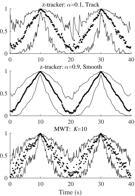
3.2. Scenario 1. Twenty second linear increase-decrease in target coherence.

Figure 2 shows the target and estimated coherence for three estimates: 1) z-tracker with α = 0.1, T = 128, tracking only, 2) z-tracker α = 0.9, T = 128 with smoothing, and 3) MWT coherence with K = 10 using 6 scales per octave over the frequency range [8,256] Hz, a total of 31 scales. Z-tracker estimates are averaged over 31 frequencies covering the first half of the frequency range [7.8,250] Hz, the MWT estimate is averaged over all 31 scales. The time for the z-tracker estimate for each segment is assigned as the centre point of each segment. The same temporal decimation is used for plotting the MWT estimate. Thus, both z-tracker and MWT coherence estimates have the same frequencies in their respective averages and use the same number of time points. Also included are the upper and lower 95% point-wise confidence limits. Averaging for coherence and confidence limits is done in the z-domain. The choice of α = 0.1, tracking and α = 0.9, smoothing represent the two

extremes in terms of the level of smoothing applied to the single segment coherence estimates. Qualitatively the additional smoothing in the latter estimate is clear in figure 2. Also visible in the tracking only estimate is the lag introduced by the Kalman filter, the estimated coherence can lag slightly behind the target coherence in figure 2 (top).

0 10 20 30 40

0 0.5

1 z-tracker: α=0.1, Track

0 10 20 30 40

0 0.5

1 z-tracker: α=0.9, Smooth

0 10 20 30 40

Time (s)

0 0.5

1 MWT: K=10

Figure 2. Single trial coherence estimates with target coherence modulated over range [0 1] with 20 second time scale. Estimates shown for 40 of the 200 seconds. (Top) z-tracker estimateα= 0.1,T = 128, tracking only, averaged using 31 frequencies over range [7.8,250] Hz. (Middle) z-tracker estimate α= 0.9, T = 128, smoothed and averaged over same frequency range. (Lower) Multiwavelet estimate withK= 10 averaged using 31 scales over frequency range [8,256] Hz at 6 scales/octave. In all cases small dots and large dots indicate target and estimated coherence for each time point, respectively. Solid lines are average upper and lower point-wise confidence limits for estimates.

frequency estimates still capture the modulation of the target coherence over the 20 second time frame.

0 10 20 30 40

0 0.5

1 z-tracker:

α=0.9, Smooth

0 10 20 30 40

Time (s)

0.5

1 MWT: K=10

0 10 20 30 40

0 0.5

1 z-tracker:

α=0.1, Track

Figure 3.Single trial, single frequency coherence estimates for 20 second coherence modulation. Same layout and parameters as figure 2.

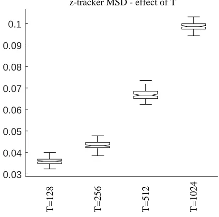
The performance of the z-tracker is quantified using an MSD metric calculated from the estimated and target coherence at each time point. First we consider the effect of changing the segment length

T. Figure 4 shows boxplots of the MSD, generated as a single MSD measure for each of the 100 trials from the z-tracker coherence estimate averaged over all frequencies and over all segments. Box plots are shown using a standard layout [32], with boxes extending from the 25th to 75th percentiles and a horizontal line at the median. Vertical lines with whiskers indicate the extremes of the data. Individual outliers are shown as

0₊0_{. Notches are included which indicate approximate}

95% confidence limits for the median, allowing visual comparison of different configurations.

It is clear that the MSD decreases monotonically as T reduces. Thus, for the broad-band target coherence in this example, frequency resolution can be sacrificed to obtain a more accurate estimate using shorter segment lengths. We did not consider segment lengths smaller thanT = 128, the frequency resolution

0.03 0.04 0.05 0.06 0.07 0.08 0.09 0.1

z-tracker MSD - effect of T

T=128 T=256 T=512 T=1024

Figure 4.Box plots of the MSD between target and estimated coherence for the z-tracker applied to the 20 second ramp increase/decrease data. Other parameters are α = 0.9 with smoothed estimates. Box plots constructed from 100 repeats with MSD calculated for average over all frequencies and over all segments for each trial.

for the assumed sampling rate of 1000/sec is ∼8 Hz, which is towards the upper end of that typically used in Fourier based analyses of neurophysiological data.

Next we consider a fixed segment length,T = 128, and look at the effects of varyingαin equation 7. The range of values is 0 < α < 1, we use the four values 0.1, 0.37, 0.61, 0.9. Low values ofαgive greater weight to the instantaneous process noise, making the filter more responsive to the residual error. Larger values of α give greater weight to previous data providing more smoothing. The intermediate values represent time constants of 1 and 2 time bins respectively in the exponential smoothing applied in equation 7.

with smoothed estimate. This has an MSD that is around 40% smaller than the MWT estimate with

K= 10.

0.04 0.05 0.06 0.07 0.08 0.09 0.1

MSD: z-tracker and MWT, 20 sec ramp.

α

=0.1 T

α

=0.37 T

α

=0.61 T

α

=0.9 T

α

=0.1 S

α

=0.37 S

α

=0.61 S

α

=0.9 S

MWT K=5 MWT K=10

Figure 5.Box plots of the MSD between target and estimated coherence for z-tracker and MWT coherence estimates applied to the 20 second ramp increase/decrease data. Other parameters are T = 128 for the z-tracker and K = 5, K = 10 for the MWT estimates. Box plots constructed from 100 repeats with MSD calculated for average over 31 frequencies/scales for the z-tracker/MWT and over all 1562 segments for each trial. MSD shown for four values ofα, with the suffixT indicating tracking and the suffixSindicating smoothing.

Single frequency MSD plots are shown in figure 6 for z-tracker with T = 128, α = 0.9 with smoothing and for MWT with K = 10. Frequency dependent effects can be seen for both types of estimate, the MSD is larger for the lowest frequency shown in the z-tracker, this is also the fundamental frequency in the single segment multi-taper coherence estimates. For MWT estimates the MSD tends to have smaller variability as the frequency increases. The single frequency MSD for the MWT estimate is around 7% lower than that for the z-tracker.

3.3. Scenario 2. Two second linear increase-decrease in target coherence.

This section describes a similar analysis to section 3.2 applied to surrogate data using a 2 second cycle time for the linear increase and decrease in the target coherence. Each trial has 200000 data points, assumed duration 200 seconds, which includes 100 repetitions of the two second triangular coherence modulation. Figure 7 shows z-tracker and MWT coherence estimates over the first 10 seconds using averaging over frequencies with the same parameters

0.12 0.14 0.16 0.18

MSD - z-tracker, single frequency

7.8 Hz 15.6 Hz 31.25 Hz 62.5 Hz 125 Hz 250 Hz

0.12 0.14 0.16 0.18

MSD - MWT, single frequency

8 Hz 16 Hz 32 Hz 64 Hz 128 Hz 256 Hz

Figure 6. Single frequency MSD box plots for (Upper) z-tracker, and (Lower) MWT coherence estimates applied to the 20 second ramp increase/decrease data. For the z-trackerT = 128, α = 0.9, with smoothing. For MWT estimates K = 10. Box plots constructed from 100 repeats with MSD calculated for individual frequencies using average over all 1562 segments/time points for each trial. MSD shown using same vertical axes.

and layout as figure 2. Figure 8 shows single frequency plots using the same layout as figure 3.

MSD box plots using the average across frequen-cies are shown in figure 9 using the same parameters and layout as figure 5. MSD box plots for single fre-quencies are shown in figure 10 using the same param-eters and layout as figure 6.

0 2 4 6 8 10 0

0.5

1 z-tracker: α=0.1, Track

0 2 4 6 8 10

0 0.5

1 z-tracker: α=0.9, Smooth

0 2 4 6 8 10

Time (s)

0.5

1 MWT: K=10

Figure 7. Single trial coherence estimates with target coherence modulated over range [0 1] with 2 second time scale, averaged over frequencies. Estimates shown for 10 of the 200 seconds. Parameters and layout same as figure 2.

has a lower MSD than the z-tracker (figure 9), the MWT estimate withK= 10 has an MSD that is 23% lower than the z-tracker withα= 0.9 with smoothing. The MSD values are larger (160% for z-tracker; 21% for MWT) than those for scenario 1 in figure 5. The MWT estimate has a clear frequency dependent effect for single frequency MSD metrics, figure 10 (lower), reflecting the scale dependent time-frequency bandwidths of the continuous wavelets. The single frequency MSD for the z-tracker, figure 10 (upper), is similar to scenario 1 in terms of any frequency dependency.

3.4. Scenario 3. Linear increase and step decrease in target coherence.

This scenario considers the ability of the z-tracker and MWT estimates to detect changes in coherence over different time scales. In this case the target coherence consists of slow increases and step decreases. The increase has the same rate of change as in scenario 1, the step decrease occurs over 1 time step, 1 ms. The transition points are determined randomly, with a

0 2 4 6 8 10

0 0.5

1 z-tracker: α=0.1, Track

0 2 4 6 8 10

0 0.5

1 z-tracker: α=0.9, Smooth

0 2 4 6 8 10

Time (s)

0.5

1 MWT: K=10

Figure 8. Single trial, single frequency coherence estimates for 2 second coherence modulation. Same layout and parameters as figure 3.

0.08 0.1 0.12 0.14 0.16

MSD: z-tracker and MWT, 2 sec ramp.

α

=0.1 T

α

=0.37 T

α

=0.61 T

α

=0.9 T

α

=0.1 S

α

=0.37 S

α

=0.61 S

α

=0.9 S

MWT K=5 MWT K=10

0.15 0.2 0.25

MSD - z-tracker, single frequency

7.8 Hz 15.6 Hz 31.25 Hz 62.5 Hz 125 Hz 250 Hz

0.15 0.2 0.25

MSD - MWT, single frequency

8 Hz 16 Hz 32 Hz 64 Hz 128 Hz 256 Hz

Figure 10.Box plots of the MSD between target and estimated coherence for z-tracker and MWT coherence estimates applied to the 2 second ramp increase/decrease data for single frequencies. Same layout and parameters as figure 6. MSD shown using same vertical axes plotting.

uniform distribution in target coherence of [0.8,1.0] for the end of the ramp and [0,0.2] for the end of the step decrease. Each trial contains 10 repetitions with 86588 data points, 86.6 seconds. Figure 11 shows z-tracker and coherence estimates for 20 seconds from one trial using averaging over frequencies. The z-tracker and wavelet estimates both capture the slow increase and sudden decrease in target coherence. The smoothing over segments in the z-tracker estimate, withα= 0.9 can be seen prior to the onset of the step decrease.

MSD metrics, calculated using the same approach as scenarios 1 and 2 from 100 trials, are shown in figure 12. These indicate that the z-tracker, with smoothing, has lower MSD than the MWT estimates, and for this configuration a lower value ofαcan reduce the MSD. A lower value ofαis likely to improve the performance of the z-tracker around the step changes in the target coherence.

0 5 10 15 20

0 0.5

1 z-tracker: α=0.1, Track

0 5 10 15 20

0 0.5

1 z-tracker: α=0.9, Smooth

0 5 10 15 20

Time (s)

0.5

1 MWT: K=10

Figure 11. Single trial coherence estimates with coherence modulated with slow increase and step decrease with averaging across frequencies. The increase in target coherence has the same rate as scenario 1, figure 2, the step decrease occurs over 1 time step, 1 ms. Parameters and layout same as figure 2.

3.5. Using Pl to characterize the variability of

z-tracker estimates.

The coherence estimates in figures 2-3, 7-8, 11 include point-wise confidence limits. These help characterise the variability associated with different estimates. For the z-tracker confidence limits are derived from the Kalman filter output, equation 9. This section examines how Pl changes with the different z-tracker

configurations for scenario 1, and compares the Kalman filter error Pl with var{zˆ} for the two MWT

estimates. Figure 13 shows box plots of the median

Pl for the 8 configurations of the z-tracker used on

scenario 1, for each of the 100 trials a single Pl,

0.04 0.06 0.08 0.1

MSD: z-tracker and MWT, ramp + step change

α

=0.1 T

α

=0.37 T

α

=0.61 T

α

=0.9 T

α

=0.1 S

α

=0.37 S

α

=0.61 S

α

=0.9 S

MWT K=5 MWT K=10

Figure 12.Box plots of the MSD between target and estimated coherence for z-tracker and MWT coherence estimates applied to the slow ramp increase and step decrease data with averaging across frequencies. Same layout and parameters as figure 5.

0.06 0.08 0.1 0.12

z-tracker: median P l

α

=0.1 T

α

=0.37 T

α

=0.61 T

α

=0.9 T

α

=0.1 S

α

=0.37 S

α

=0.61 S

α

=0.9 S

MWT K=5 MWT K=10

Figure 13.Box plots of the medianPlfor the 100 repeat runs in scenario 1 using the 20 second ramp increase/decrease in target coherence. Horizontal lines for the MWT estimates show the fixed values ofvar{ˆz}forK= 5 andK= 10.

Using a single value of Pl to represent the

variability for each run does not provide any information regarding the distribution across segments in each trial. Figure 14 shows a histogram of the distribution ofPl for a single trial in scenario 1 across

the 1562 segments with T = 128 and α = 0.9 with smoothing. The distribution has a positive skew, this is likely to reflect the adaptive nature of the Kalman filtering. When a large residual triggers an increase in the filter gain the error will also increase transiently. For the MWT estimate with K = 10, var{zˆ}= 0.56, this is close to the peak in the distribution ofPl.

0.02 0.04 0.06 0.08 0.1 0.12 0.14 0.16 0.18 0.2

P l

0 0.02 0.04 0.06 0.08 0.1 0.12 0.14

P

l over segments, α=0.9 S

Figure 14. Normalised histogram ofPlover 1562 segments in a single trial for scenario 1 with configurationα= 0.9, smoothing. The value ofvar{ˆz}for the MWT estimate withK= 10 is 0.56.

3.6. Testing for zero coherence.

An important aspect of coherence analysis is testing for a null hypothesis of zero coherence. In this section we examine the behaviour of the z-tracker when applied to surrogate data with no correlation. Simulated data of length 200000 samples, assumed sampling rate 1 ms, generated using equations 10, 11 withβt= 0 anddt=

1 gives a target coherence of zero, for all frequencies. Figure 15 compares the z-tracker coherence estimate,

limit for the MWT estimate uses the expression in [8]. Both estimates exhibit a similar range of values, with no obvious bias over time from the z-tracker estimate.

0 10 20 30 40

0 0.1 0.2 0.3

0.4 z-tracker:

α=0.9, Smooth

0 10 20 30 40

Time (s)

0.1 0.2 0.3

0.4 MWT: K=10

Figure 15. Single trial z-tracker (T = 128, α = 0.9 with smoothing) and MWT (K = 10) coherence estimates for uncorrelated stationary Gaussian data. Estimates are averaged over 31 frequencies, using the same frequencies as figure 2.

Determined empirically for each z-tracker config-uration, using the approach of taking the 5% point of the distribution of estimated coherence values across 100 repeat runs and across all frequencies, gives a range of values for the 95% confidence limit of 0.475 for

T = 128,α= 0.1 with tracking to 0.25 formT = 1024,

α = 0.9 with smoothing. These empirical confidence limits decrease asT is increased and as αis increased and are lower for smoothing than tracking. For com-parison using the expression in [8] to determine con-fidence limits, using the complex degrees of freedom for each MWT estimates give 95% confidence limits of 0.53 for K = 5 and 0.28 for K = 10. Although ex-pressions to estimate the complex degrees of freedom of the z-tracker have not been developed, this compar-ison suggests that the two approaches, with parameter values as used in the present study, have similar ranges for their complex degrees of freedom.

To quantify the relative performance of the z-tracker against the benchmark MWT estimate, figure 17 shows boxplots of MSD estimates generated as a single MSD measure for each of the 100 trials for two z-tracker estimates (T = 128 and T = 1024, both

0 10 20 30 40

0 0.2 0.4

0.6 z-tracker:

α=0.9, Smooth

0 10 20 30 40

Time (s)

0 0.2 0.4

0.6 MWT: K=10

Figure 16. Indicative single frequency coherence estimates, using the median frequency for the same data and same analysis parameters as in figure 16. Upper trace is z-tracker estimate, Lower trace is MWT estimate. The horizontal dashed lines are the upper 95% confidence limits for a null hypothesis of uncorrelated data, determined empirically for the z-tracker and using the expression in [8] for the MWT estimate.

with α = 0.9) and two MWT (K = 5 and K = 10) estimates.

The box plots in figure 17 suggest that the performance of the z-tracker on uncorrelated data is similar to that of MWT based estimates. For this data a longer segment length leads to lower MSD values for the z-tracker.

3.7. Experimental data.

0.05 0.1 0.15

MSD - zero coherence

T=128 T=1024 K=5 K=10

Figure 17. Box plots of the MSD for target coherence of zero for two z-tracker (T = 128 and T = 1024) and two MWT (K= 5 andK= 10) coherence estimates. Other parameters are α= 0.9 with smoothing for the z-tracker estimates. Box plots constructed from 100 repeats with MSD calculated for average over 31 frequencies/scales for the z-tracker/MWT and over all 1562 segments forT = 128 z-tracker and over all 195 segments for T = 1024 z-tracker. MSD for MWT use 195 time points matching the midpoint of segments for theT = 1024 z-tracker.

estimates it was found that the mPFC-BLA coherence after the final dose was significantly lower than the coherence prior to the first dose at frequencies <2Hz [45]. The aim in applying the z-tracker to this data is to get additional insight into the time scales of these changes in coherence. Figure 18 shows the z-tracker coherence estimate over the 990 second record with configuration T = 1024, α = 0.9 with smoothing. The choice ofT is motivated by the need to examine frequencies<2Hz, and the choice ofαis motivated by the MSD results in figure 5.

A reduction in the coherence after the first dose of the agonist can be seen in the heat map in figure 18(Upper). The section at frequency 0.98Hz, the lowest frequency bin, figure 18(Lower), quantifies this change over time. Following each dose of the agonist there is a marked reduction in coherence, this is most prominent following the first dose, when the coherence is abolished around 330 seconds. Following the final dose there is no obvious reduction in coherence. Prior to the first dose the mean coherence at 1 Hz is 0.78, the mean coherence from 60 seconds after the last dose until the end of the record is 0.64. Thus, for this example, the z-tracker is able to give additional insight into changes in coherence over time, and appears to detect changes in single frequency components, figure 18(Lower).

3.8. Computational complexity of z-tracker and multiwavelet algorithms.

One factor in the choice of algorithm to use to estimate time-varying coherence is the computational complexity of the different approaches. Here we consider briefly the computation time of the two methods, focusing on a comparison of the time to compute the necessary Fourier transforms using an FFT algorithm, and using a comparison of the run time on the same data.

The algorithms are implemented in MATLAB [31], which uses an FFT algorithm with computing time of order O(NlogN) for an FFT with N points, this is independent of the value of N [22]. Using this expression we can compare the computational time to compute the Fourier coefficients for the z-tracker and MWT algorithms. The MWT algorithm uses an FFT based convolution to calculate the wavelet coefficients at each scale, this is achieved with an inverse Fourier transform, we assume the computation time for forward and inverse Fourier transforms is the same. The following comparison is based on scenario 1, section 3.2, which uses bivariate data of length 2×105 points. Considering the z-tracker with segment size

T = 128 and L= 1562 segments, a bivariate analysis for single segment coherence estimates with K = 2 multitaper windows will have computing time of order

O(4L T logT) = O 3.9×106

. The MWT estimate, using K = 10 orthogonal Morse wavelets applied to the complete recordN = 2×105 _usingN

s= 31 scales

will require Fourier transforms with computing time of order O(2Ns (K+ 1) N logN) = O 1.6×109.

These figures suggest that the z-tracker will be 2-3 orders of magnitude faster in execution time than the multiwavelet analysis. However, the z-tracker has a number of additional steps that must be performed for each segment according to the algorithm in section 2.2. In a comparison of execution times in MATLAB, comparing 100 runs on scenario 1 data, the z-tracker is about 50 times faster than the multiwavelet analysis. Thus, if execution time is an important factor in any analysis the z-tracker may be preferred to multiwavelet analysis.

4. Discussion

mPFC - BLA coherence. T=210, α=0.9

0 100 200 300 400 500 600 700 800 900

45 40 35 30 25 20 15 10 5

Frequency (Hz)

0.4 0.6 0.8

0 100 200 300 400 500 600 700 800 900

Time (s)

0.2 0.4 0.6 0.8 1

Coherence

mPFC - BLA coherence: 1 Hz. T=210, α=0.9

Figure 18. Analysis ofin-vivorecording of local field potentials from mPFC and BLA in anaesthetized rat during an experiment to mimic increased stress pharmacologically. Four doses of a stress agent were applied at 216, 420, 602 and 840 seconds into the recording. (Upper) Heat map of z-tracker coherence estimate over the 990 second record,T = 1024,α= 0.9 with smoothing, using 966 segments. Colour bar to the right indicates coherence magnitude. (Lower) Section with coherence estimate at lowest frequency bin, 0.98 Hz. Solid line indicates coherence estimate, grey lines are upper and lower 95% point-wise confidence limits. Vertical dotted lines indicate times at which stress agent was administered.

than expected residual terms. This allows the filter to respond rapidly to sudden increases or decreases in the correlation. In contrast if the correlation is relatively constant or slowly changing the Kalman filter can apply greater levels of local smoothing, helping to reduce variability.

The performance of the z-tracker was explored using surrogate data and compared with wavelet coherence using an MSD metric. For data with slowly varying target coherence, including occasional step changes, the z-tracker exhibited a lower MSD than MWT coherence. For more rapidly changing target coherence a MWT estimate gave a lower MSD than the z-tracker. The two parameters to consider in a z-tracker analysis are the segment size, T, and the smoothing to apply to the Kalman filter noise sequence, using parameter α, with larger α resulting in greater smoothing. Using shorter segment sizes reduced the MSD as did a larger value ofα. An exception to this was data with sudden changes in coherence, when a smaller value ofαgave a lower MSD. In addition, when testing for zero coherence increasing the segment size reduced the MSD. Analysis of in vivo experimental LFP data demonstrated the potential of the method to provide insight into modulation of coherence over time.

To our knowledge this is the first attempt

at combining multi-taper spectral estimates with adaptive Kalman filtering to estimate correlation over time. It builds on our earlier work using adaptive Kalman filtering in the univariate case for spectral estimation [10] and non-adaptive Kalman filtering with Periodogram based spectral estimates. Auto and cross spectral estimates were tracked separately over segments with Kalman filtering/smoothing, and combined to estimate coherence for each segment [9]. The advantage of the z-tracker is that only a single set of frequency components are used in the Kalman filtering step. In addition the assumption of constant variance for thelogeof the real and imaginary

components of the cross spectrum used in [9] apply only when the coherence is zero, this may introduce an additional bias into estimates which have non-zero coherence. This does not apply to the z-tracker which instead works with a single set of frequency values in thezdomain.

Several aspects of the z-tracker are worthy of further study. We have used only one configuration for estimation of the single segment coherence estimates in equation 3, with N W = 1.5, K = 2, the bias and variance lookup tables apply only to this case. Further lookup tables could be generated for increased

segments uses increased process noise variance to increase the Kalman gain, this is triggered by larger than expected residual, equation 6. In the estimation ofq_l0we used all frequency points (apart from zero and nyquist), in some cases it may be more appropriate to use a restricted range of points to estimate the residual variance.

This study considers only time series data. Extending the approach to point-process data would open up further applications in, for example, analysis of multielectrode array recordings of single unit data. A possible route here would be to consider the approach to point-process analysis in [24], which allows analysis of time series and point process data in a combined framework.

The z-tracker uses an empirical approach in the z-domain with coherence estimates and point-wise confidence limits derived from the Kalman filter output. Confidence limits for a null hypothesis of zero coherence are derived empirically using mote-carlo methods. The success of the method will rely, in part, on the accuracy of the assumptions made regarding the applicability of the Kalman filter in thez-domain. Comparison with the multiwavelet coherence suggests these assumptions are reasonable. One advantage of wavelet coherence is the theoretical work which has derived expressions for the statistical distribution facilitating hypothesis testing [17]. Further work is required to develop a similar level of statistical rigour for the z-tracker. A possible approach is to re-formulate the z-tracker as a weighted overlapping segment average (WOSA) estimate, as used for temporally smoothed wavelet coherence estimates [18]. Our recommendations for the choice of z-tracker parameter α are based on an MSD metric. An alternative theoretical treatment could consider a likelihood expansion of the Kalman filter state and observation models to choose α using maximum likelihood over the range forα, e.g. [37].

The z-tracker provides a computationally efficient approach, around 50 times faster in our MATLAB implementation, for analysis of correlation in long records which can be sectioned into short segments. Applications include comparison of baseline activity vs stimulus-induced changes in activity as in figure 18. The method is also suitable for more exploratory analyses, for example investigating the consistency of correlation over time. In experiments involving repeat trials over time the method could be used to characterise changes in coherence from trial-to-trial, with the Kalman filter error used to quantify the uncertainty across trials. The data adaptive nature of the algorithm should also open up new approaches in coherence estimation for non-stationary data in other fields.

5. Software toolbox

A software toolbox in MATLAB to undertake the analysis in this paper is freely available at http:// www.neurospec.org/. The software includes a user guide and example scripts.

Acknowledgments

The authors would like to thank the referees for their helpful comments. The work of D.M. Halliday and J-S. Brittain was supported by the Biotechnology and Biological Sciences Research Council of the United Kingdom (Ref 10477).

Appendix A. Kalman filtering and smoothing.

This Appendix provides an overview of the Kalman filtering and smoothing equations as applied to the single segment coherence estimates. The Kalman filter state and observation equations are [11, 26]

xl+1=φlxl+wl, (A.1)

zl=Hlxl+vl. (A.2)

Here xl is the (unknown) vector of z-transformed

coherence at segmentl andzlis the vector containing

the single segment z-transformed estimate, equation 4, over the frequency range of interest. The vectors wl and vl are the process and observation noise with

covariance matricesQlandRl, respectively. A number

of assumptions are made concerning the characteristics of the state transition and observation matrices and the noise processes. As in our previous work [9, 10] we set φ_l=Hl=I, whereIis the identity matrix, based on

the assumption that the spectral coherence is constant from segment to segment. This random walk model with process noise provides the flexibility to deal with a range of correlation scenarios, including constant, and slowly and rapidly changing correlation from segment to segment. We assume the noise processes are zero mean, and that the process and observation noise covariance matrices can be represented as Ql = qlI

andRl=rlI, respectively.

These assumptions mean that the state and observation equations, A.1, A.2, process the coherence at each frequency independently and with the same Kalman gain, therefore the Kalman filter gain, Kl,

and error Pl are constant across all frequencies and

can be reduced to scalar quantities, denoted Kl and

Pl, respectively.

The addition of process noise,wl, allows changes

in correlation to be detected [25]. This process noise covariance, Ql = qlI has to be specified at

variability [9]. In the current adaptive framework the process noise is adjusted as each segment is incorporated allowing the Kalman filter to adapt to unusual data [10], or to apply more smoothing if the data between segments is consistent. The observation noise covariance, Rl = rlI, is determined from the

uncertainty (variance) of the single segment estimator, equation 4. Calculation of rl is described in section

2.3.

With the above assumptions, the estimate and error for segmentl, are given by [9]

xl=x p

l +Kl(zl−x p

l) (A.3)

Pl= (1−Kl)Plp. (A.4)

Here xp_l is the vector of predicted or a-priori values andP_lp is thea-priori error. The Kalman filter gain is

Kl=Plp(P p

l +rl)−1. In our formulation the predicted

error, P_lp, and corrected error, Pl, apply to all values

inxp_l andxl, respectively. The prediction steps are

xp_l+1=xl (A.5)

P_lp₊₁=Pl+ql (A.6)

whereqlis the variance of the process noise for segment

l. The filter is initialised as x1 = z1, P1 = r1. The

tracking process proceeds recursively froml= 2, . . . , L

using equations A.3, A.4.

Kalman smoothing is incorporated using the approach in [9, 42]. This implements a backward smoothing pass over the segments, starting from the final segment. Using˜xland ˜Plto represent the vector

of smoothedz-transformed coherency values and error, respectively, for segmentl the backward smoothing is implemented as

˜

xl=xl+Al(x˜l+1−xpl+1) (A.7)

˜

Pl=Pl+A2l

˜

Pl+1−Plp+1

(A.8)

where Al is the Kalman gain for the backward pass,

Al = Pl Plp+1 −1

. The smoothing process proceeds recursively froml= (L−1), . . . ,1 using equations A.7, A.8. The smoothing process is initialised as ˜xL=xL,

˜

PL =PL, the final segment is fully conditioned on all

available segments after tracking.

Appendix B. Algorithmic description of z-tracker.

This Appendix contains an algorithmic level descrip-tion of the z-tracker, with reference to the relevant equations or sections.

References

[1] Addison PS (2002) The Illustrated Wavelet Transform Handbook. Institute of Physics, Bristol.

Algorithm 1z-tracker Input: x, y, L, T, α

Output: |Rˆyx(λj, l)|2

1: Initialize: Calculate ˆz1, r1. P1=r1, K1= 1, q1= 0 2: forl= 2 toLcalculate:

3: ˆzl, equation (4) 4: rl, section (2.3) 5: xp_l, equation (A.5)

6: q_l0, equation (6)

7: ql, equation (7) 8: P_lp, equation (A.6)

9: Kl, xl, Pl, equations (A.3, A.4) 10: end for

11: Initialize reverse pass: ˜xL=xl,p˜L =pl 12: forl=L−1to1 calculate:

13: Al,x˜l,P˜l, equations (A.7, A.8) 14: end for

15: Bias correction, map to coherence: equation(8)

[2] Baraniuk RG, Bayram M (2000) Multiple Window Time Varying Spectrum Estimation. In: Nonlinear and Nonstationary Signal Processing, eds Fitzgerald WJ, Smith RL, Walden AT, Young P. Cambridge University Press, Cambrige. pp 292 - 313.

[3] Ba D, Babadi B, Purdon PL, Brown EN (2014). Robust spectrotemporal decomposition by iteratively reweighted least squares. Proceedings of the National Academy of Sciences, 111(50), E5336-E5345.

[4] Bloomfield P (2002) Fourier analyis of time series - An introduction, 2nd ed. John Wiley & Sons Inc. New York. [5] Bokil H, Purpura K, Schoffelen J-M, Thomson D, Mitra P (2007). Comparing spectra and coherences for groups of unequal size. Journal of Neuroscience Methods, 159: 337-345.

[6] Brillinger DR (1974) Fourier analysis of stationary processes. Proceedings of the IEEE, 62: 1628-1643. [7] Brillinger DR (1975) Time Series - Data Analysis and

Theory. Holt Rinehart & Winston Inc. New York. [8] Brittain J-S, Halliday DM, Conway BA, Nielsen JB (2007)

Single-trial multiwavelet coherence in application to neurophysiological time series. IEEE Transactions on Bio-Medical Engineering, 54(5), 854-62.

[9] Brittain J-S, Catton C, Conway BA, Nielsen JB, Jenkinson N, Halliday, DM (2009) Optimal spectral tracking-with application to speed dependent neural modulation of tibialis anterior during human treadmill walking. Journal of Neuroscience Methods, 177(2), 334-347.

[10] Brittain J-S, Halliday DM (2011) Optimal spectral tracking-Adapting to dynamic regime change. Journal of Neuroscience Methods, 195(1), 111-115.

[11] Brown RG, Hwang PYC (1997) Introduction to Random Signals and Applied Kalman Filtering, 3rd ed. John Wiley & Sons, New York.

[12] Bruns A (2004) Fourier-, Hilbert- and wavelet-based signal analysis: are they really different approaches? Journal of Neuroscience Methods, 137(2), 321-332.

[13] Carter GC (1987) Coherence and time delay estimation. Proceedings of the IEEE, 75(2), 236-255.

[14] Carter GC, Knapp C, Nuttall A (1973) Statistics of the estimate of the magnitute-coherence function. IEEE Transactions on Audio and Electroacoustics, 21(4), 388-389.

magnitude-squared coherence function via overlapped fast Fourier transform processing. IEEE Transactions on Audio and Electroacoustics, 21(4), 337-344.

[16] Chronux.org (2017). [online] Available at: http://chronux.org/ [Accessed 19 Dec. 2017].

[17] Cohen EAK, Walden AT (2010) A Statistical Analysis of Morse Wavelet Coherence. IEEE Transactions on Signal Processing, 58(3), 980-989.

[18] Cohen EAK, Walden AT (2010) A Statistical Study of Temporally Smoothed Wavelet Coherence. IEEE Transactions on Signal Processing, 58(6), 2964-2973. [19] Cohen EAK, Walden AT (2011) Wavelet Coherence

for Certain Nonstationary Bivariate Processes. IEEE Transactions on Signal Processing, 59(6), 2522-2531. [20] Cohen L (1995) Time-Frequency Analysis. Prentice-Hall

Inc. New Jersey.

[21] Enochson LD, Goodman NR (1965). Gaussian ap-proximations to the distribution of sample co-herence. Technical Report, AD0620987, Measure-ment Analysis Corp, Los Angelas. Available from http://oai.dtic.mil/oai/oai?verb=getRecord& metadataPrefix=html&identifier=AD0620987

[22] Frigo M, Johnson SG (2005) The Design and Implementa-tion of FFTW3. Proceedings of the IEEE, 93(2), 216-231. [23] Gabor, D (1946) Theory of communication. Part 1: The analysis of information. Journal of the Institution of Radio and Communication Engineering, 93(26), 429-441. [24] Halliday DM, Rosenberg JR, Amjad AM, Breeze P, Conway BA, Farmer SF (1995) A framework for the analysis of mixed time series/point process data - Theory and application to the study of physiological tremor, single motor unit discharges and electromyograms. Progress in Biophysics and molecular Biology, 64: 237-278. [25] Jazwinski AH (1969) Adaptive filtering. Automatica, 5(4),

475-485.

[26] Jazwinski AH (1970) Stochastic Processes and Filtering Theory. Academic Press, New York.

[27] Kalman RE (1960) A New Approach to Linear Filtering and Prediction Problems. Transactions of the ASME-Journal of Basic Engineering, 82, Series D, 35-45.

[28] Lilly JM Olhede SC (2009) Higher-Order Properties of Analytic Wavelets. IEEE Transactions on Signal Processing, 57(1), 146-160.

[29] Lilly JM Olhede SC (2010) On the Analytic Wavelet Transform. IEEE Transactions on Information Theory, 56(8), 4135-4156.

[30] Lilly JM Olhede SC (2012) Generalized Morse Wavelets as a Superfamily of Analytic Wavelets. IEEE Transactions on Signal Processing, 60(11), 6036-6041.

[31] MATLAB Release 2016a, The MathWorks, Inc., Natick, Massachusetts, United States.

[32] McGill R Tukey JW Larsen WA. (1978) Variations of Box Plots. The American Statistician, 32(1), 12-16.

[33] Milde T Leistritz L Astolfi L Miltner WHR Weiss T Babiloni F Witte H (2010) A new Kalman filter approach for the estimation of high-dimensional time-variant multivariate AR models and its application in analysis of laser-evoked brain potentials. NeuroImage, 50(3), 960-969.

[34] M¨oller E Schack B Arnold M Witte H (2001) Instantaneous multivariate EEG coherence analysis by means of adap-tive high-dimensional autoregressive models. Journal of Neuroscience Methods, 105(2), 143-158

[35] Nielsen JB, Conway BA, Halliday DM, Perreault M-C, Hultborn H (2005) Organization of common synaptic drive to motoneurones during fictive locomotion in the spinal cat. Journal of Physiology, 569, 291-304.

[36] Olhede SC, Walden AT (2002) Generalized Morse wavelets. IEEE Transactions on Signal Processing, 50: 2661-2670. [37] Ostwald D, Kirilina E, Starke L, Blankenburg F (2014) A

tutorial on variational Bayes for latent linear stochastic time-series models. Journal of Mathematical Psychology, 60, 1-19.

[38] Percival DB, Walden AT (1993) Spectral Analysis for Physical Applications. Cambridge Univ. Press, UK. [39] Priestley MB (1981) Spectral analysis and time series.

Academic Press, London.

[40] Priestley MB (1988) Non-linear and Non-stationary Time Series Analysis. Academic Press, London.

[41] Priestley MB (1996) Wavelets and Time-dependent Spec-tral Analysis. Journal of Time Series Analysis, 17(1), 85-103.

[42] Rauch HE, Tung F, Striebel CT (1965) Maximum likelihood estimates of linear dynamic systems. AIAA Journal, 3(8), 1445-1450.

[43] Rosenberg JR, Amjad A, Breeze P, Brillinger DR, Halliday DM (1989). The Fourier approach to the identification of functional coupling between neuronal spike trains. Progress in Biophysics and Molecular Biology, 53: 1-31. [44] Siegel M, Donner TH, Engel AK (2012) Spectral finger-prints of large-scale neuronal interactions. Nature Re-views Neuroscience, 13(2), 121-134.

[45] Stevenson CW, Halliday DM, Marsden CA, Mason R (2007) Systemic administration of the benzodiazepine receptor partial inverse agonist FG-7142 disrupts corticolimbic network interactions. Synapse, 61(8), 646-663.

[46] Thomson DJ (1982) Spectrum estimation and harmonic analysis. Proceedings of the IEEE, 70: 1055-1096. [47] Thomson DJ, Chave A (1991) Jackknifed error estimates

for spectra, coherences, and transfer functions. In S. Haykin (Ed.), Advances in spectrum analysis and array processing, 1. pp 58-113.

[48] Torrence C, Compo G (1998) A practical guide to wavelet analysis. Bulletin of the American Meteorological Society, 79(1), 61-78.

[49] Walden AT, Cohen EAK (2012) Statistical Properties for Coherence Estimators From Evolutionary Spectra. IEEE Transactions on Signal Processing, 60(9), 4586-4597. [50] Welch P (1967) The use of fast Fourier transform for

the estimation of power spectra: a method based on time averaging over short, modified periodograms. IEEE Transactions on Audio and Electroacoustics, 15(2), 70-73.