Network models of three dimensional electromagnetic fields

Technical article

Network models of three-dimensional electromagnetic fields

I. INTRODUCTION

One of the oldest techniques for electromagnetic field analysis and computation relies on magnetic and/or electric field equivalent circuits. Historically such circuits tended to be simple with few degrees of freedom due to limitations to available computing power and memory; notwithstanding, these methods are still helpful in providing efficient estimates of global parameters and are used for teaching purposes as they are well based physically and avoid complicated mathematical descriptions. They are also used in real time simulations and for analysis of complex structures. Dramatic increases in computer speed and available memory have removed many restrictions and progressively more accurate models are being used based mainly on the finite element (FE) formulations.

The principal advantage of the equivalent networks is that they provide useful physical insight and rely on well known and understood Kirchhoff’s and Ohm’s laws for electric and magnetic circuits [6, 16, 18]. The solution uses methods from circuit theory which are generally considered by engineers as much simpler than finite element formulations. It is therefore not surprising that researchers have long been searching for analogies between field descriptions and network equivalents.

The authors have for many years taught courses on finite elements and have developed a network description of the FE formulation which allows the method to be explained using the language of circuit theory [7, 8, 9, 11]. This article presents briefly such an approach, discusses the use of potentials and shows various possible descriptions of the elements using nodal, edge, facet and volume formulations. An 8-node hexahedron is used to illustrate the implementation of the general ideas.

II. ELECTROMAGNETIC FIELD EQUATIONS The electromagnetic field may be described using the usual set of equations

J H =

curl , curlE=−∂B ∂t (1a,b)

B

H =ν , J=σE+∂(eE) ∂t (2a,b)

where the expression for current density refers to two components: conduction (using conductivity s of material) and displacement current due to time variation of the electric field. For brevity we introduce the notation

E

J=γ (3)

where γ=σ+pε (and p=∂/∂t) contains both components and may be referred to as ‘operational’ conductivity.

In wave problems an alternative to (1a) is often used, in which current density is expressed in terms of a time derivative of an electric flux density D, which yields

t ∂ ∂

= D

H

rot , while D=ε_pE, and an ‘operational’

electric constantε_p=p−1γ=p−1σ+ε.

From (1b) it follows that divB=0, as there may be no ‘free’ magnetic poles, and from (1a) we can deduce divJ=0, which expresses the law of conservation of charges in the absence of free electric charge (in other words the continuity of conduction current, or the field equivalent of Kirchhoff’s current law). The equations divB=0 and divJ=0, together with (1a) or (1b), are normally used when the magnetic and electric fields are considered separately, for example when seeking field distributions due to imposed current density or solving equations describing current density distributions resulting from time variation of the prescribed flux density.

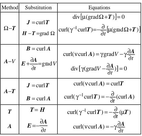
Electromagnetic fields may be solved using field equations directly (H, B, E or D) or by introducing potential functions. The potential formulations are considered more general and will be discussed here. There are three main approaches based on potentials: (a) the Ω−T method, where the magnetic field is expressed in terms of a scalar potential Ω, while the electric field is described using an electric vector potential T; (b) the A−V formulation, where A is a magnetic vector potential and V an electric scalar potential; and (c) the A−T formulation based on magnetic and electric vector potentials.

Table I. Equations for the different potential formulations

Method Substitution Equations

Ω−T

T J =curl

Ω = −T grad H

[

]

div µ Ω+T =

[

]

) curl

curl( 1 T µ Ω+T

∂∂ − = γ−

t

A−V

A B=curl

V t =grad ∂ ∂ + A

E t

V ∂ ∂ γ − γ =

ν_{curlA) grad} A

curl(

0 ) (grad

div

[

]

∂ ∂ − γ

t

V A

A−T

T J =curl

A B=curl

T A) curl curl

curl(ν =

) (curl )

curl

curl( 1 T A

t ∂∂ − = γ−

T

A

H T=

t ∂ ∂ −

= A

E

) ( ) curl

curl( 1 T µT

∂∂ − = γ−

t

t ∂ ∂ γ − =

ν_curlA) A

curl(

may not always be necessary [2, 7, 17]. By using numerical techniques such as relaxation methods or ICCG, one of the possible solutions is found satisfying the equations for potentials. Finding one of the solutions may be faster than searching for the only one satisfying the gauge conditions [2, 17].

The following discussion concentrates on the ungauged solutions. Using the language of the circuit theory, the finite element method is derived for all three potential formulations.

III. FINITE ELEMENT INTERPOLTATION FUNCTIONS A final element may be considered as nodal, edge, facet or volume [3, 9, 12]. In the nodal formulation the distribution of a scalar quantity inside an element is expressed in terms of the values at nodes (e.g. vertices). An edge element describes a vector quantity in that element through the values of integrals of this quantity along the element edges – these integrals are known as edge values. In a facet element the function describing a distribution of a vector quantity inside is associated with the surface integrals of that quantity on the element facets – the integrals are known as facet values. Finally, a volume element may be defined if a distribution of a scalar quantity is expressed in terms of known volume integrals of this quantity – the integrals are called the volume values. As a consequence of the multiplicity of integration, a volume element may be referred to as an element of the third order, a facet element as second order, an edge element as first order and a nodal element as zero order. For the element of the ith order we can write

∑

= ni j

j i j i

i w y

y 1

, ,

(i = 0, 1, 2, 3) (4) where yi,j is the jth nodal value for i=0, edge value for i=1, facet value for i=2 and volume value for i=3; wi,j is

the jth interpolating function of the element of the ith order; and ni is the number of values of the field quantity yi (ni equals the number of nodes for i=0, the number of

edges for i=1, the number of facets for i=2 and the number of volumes for i=3; typical elements have one volume, hence n3=1). The interpolating functions for

elements of third and zero order are scalar. Equation (4) may be written in a matrix form

i i i

y =wY (i= 0, 1, 2, 3) (5) Here wi is a matrix of interpolating functions of the

element of ith order, and Yi a vector of associated values,

e.g. a vector of nodal (i=0), edge (i=1), facet (i=2) or volume (i=3) values. The values and interpolating functions of the edge and facet elements, that is elements of the first and second order, are vectors; accordingly they are further designated using bold letters.

As the field quantities describing magnetic fields, as well as their sources, are themselves vectors, it is often beneficial to use interpolating functions which are also vectors and thus make the best use of edge and facet elements.

IV. FINITE ELEMENT GRAPHS

In electromagnetic field systems the functions w1,j of

the edge element are used to describe: (a) a gradient of the electric, V, or magnetic, O, scalar potential, (b) electric or magnetic field strength, or (c) electric, T, or magnetic, A, vector potentials. The functions w2,j of the

facet element, on the other hand, are related to the current density J or the magnetic flux density B. The edge values of the relevant field intensities represent voltages, whereas the edge values of the vector potentials T and A are linked with the loop currents and fluxes around the edge, respectively. The facet value of J is a current, while the facet value of B is a flux through the facet [9].

Let a vector quantity y1 be expressed in terms of a

gradient of a scalar y0, i.e. y1=grady0. Hence the edge

value y1,j for the jth edge, with the start at Pp and the end

at Pq, may be written as

) ( ) (

d 0 0

1 ,

1 q p

P

P

j y P y P

y q

p

− =

=

_∫

This relationship shows that the edge value of the gradient equals the potential difference between the edge ends. This may be written in matrix form for all edges of a finite element mesh as

0 1 k Y

Y = w (7)

where Y1 is the vector of the edge values of gra dy0, Y0 a

vector of the nodal values of y0, and kw a transposed

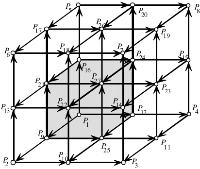
nodal matrix of a graph whose branches coincide with the edges of the discretising mesh (Fig. 1). Equation (7) is a network representation of the substitution y1=grady0. For

electromagnetic systems Y1 becomes a vector of branch

voltages and Y0 a vector of nodal values of a scalar

potential. For the remainder of this article, the graphs and networks with branches coinciding with the finite element mesh will be referred to as edge networks (EN) [9, 11].

P₄ P₁

P₆

P₅

P₂ P₃

P₈

P₁₄ P

7

P₉

P₁₉

P₁₂ P₁₃

P₁₅ P₁₆

P₁₇

P

18

P₂₀

P

11

P₂₄

P₂₁

P₂₂

P

23

P₂₅ P

27

P₂₆

P₁₀

Fig. 1. Edge graph of 8 hexahedrons

In the electromagnetic field analysis it is common practice to express the current and flux densities in terms of a circulation of a vector potential. The vector potentials represent a vector quantity y1 associated with

an edge element, while densities B and J correspond to a vector quantity y2 related to a facet element. Using the

facet value y2,j has been determined following the above

definition of y2 and by applying the Stoke’s theorem we

obtain

∑

q q

j y

y2, 1, (8)

Here the summation refers to the edge values of all edges of the jth facet. The sign in front of the qth edge value y1,q

depends on the direction of the qth edge. For all mesh facets we can write

1

2 kY

Y = s (9)

where Y2 is a vector of the facet values, and ks is a

transposed loop matrix of a graph whose nodes are positioned in the centre of element volumes and the branches connecting the nodes cut the facets as shown in Fig. 2. This type of graph and associated networks have been named facet networks (FN) [9, 11]. The matrix ks

refers to loops around the edges and is also the loop matrix of the edge graph where edges are linked with relevant facets. Equation (9) is a network equivalent of the substitution y2=curly1 and expresses branch values

using loop values.

Q₆

Q₁

Q₂

Q₈

Q₄ Q₅

Q₇

Q

3

Branch of adjoin element

S1

S2

S8

S3 S4 Point in centre of

element face

Network node, centre of element

Fig. 2. Facet graph of 8 hexahedrons

Table II. Network representations of differential operators

Network equivalents of the differential operations

Differential operations

Edge graph Facet graph

div y _kwT_Y1 kVY2

curl y _ksY1, kTsY2 ksY1, kTsY2

grad y kwY0 kVTY3

curlgrad y=0 kskw=0 VT =0

T sk k

div curl y=0 T =0

s T wk

k kVks=0

Referring now to the volume value y3,j of a quantity y3, considering that it is a divergence of a vector y2, and

applying Gauss theorem, leads to the following expression

∑

p p

j y

y3, 2, (10)

where the summation involves the facet values y2,p of all

facets of the jth volume. For all elements of the

discretising mesh we can write

2

3 k Y

Y = V (11)

where Y3 is a vector of volume values, and kV a matrix

of cuts of the edge graph, with cuts associated with facets. These matrices are network representations of the differential operators as explained in Table II.

V. BRANCH EQUATIONS FOR EDGE ELEMENT MODELS

The vector functions which are associated with an edge element are: the electric and magnetic field intensity, the potential gradient and the vector potentials. The edge values of these functions for the edge Ni,j with

the beginning at Pi and the end at Pj, are assembled in

Table III.

Table III. Edge values of the field vectors for an edge Ni,j with

the beginning at Pi and an end at Pj

Quantity Edge value Description of the edge value

gradV Vj−Vi Electric potential difference between _nodes gradΩ Ωj −Ωi Magnetic potential difference between

nodes

H uHNi,j

Magnetic potential associated with branch permeance

E uENi,j

Electric potential associated with operational branch admittance

A

j i N

o _,

φ Loop flux around the edge

T ioN_i,_j Loop current around the edge

Using the relationships from Table I,H−T=gradΩ

and E+∂A ∂t=gradV, it is possible to establish correlations between the edge values of Table III. Integrating both sides along the edge Ni,j leads to the

following expressions

i j oN HNi j i i j

u _, − _, =Ω −Ω (12a)

i j oN

EN t V V

u _i,j +dφ _i,j d = − (12b)

P2 P4

Pj

P6

P5

Pi

P8 P1

N3,4

Ni,j

N5,6 N2,6

N5 ,j

li,j

Vi or Ωi

Vj or Ωj uENi,j or uHNi,j

egNi,j orΘNi,j

i_{g Ni,j} orφ_{g Ni,j}

Fig. 3. An edge model of an 8-node, 12-edge element.

The implications of expressions (12a) and (12b) are as follows. The potential difference between nodes of the branch Ni,j of the edge graph (e.g. that of Fig. 3) is a sum

j i

EN

u _, or uHN_i,_jacross the branch elements (the branch Ni,j is associated with the edge Ni,j). The branch emf is

expressed in terms of the time derivative of the flux around the edge, e_gNi,j=−dφ_oNi,j dt. The branch mmf corresponds to the loop current ioi,j, Θ_Ni,j=i_oNi,j.

The current igN_i,_jin the branch Ni,j of the edge model of a single element containing an electric field may be obtained using the following expression

∫∫∫

i _, w1, _, Jd (13)

where Ve is the element volume. Equation (3) should be

used, while the E vector may be described in terms of the interpolating functions of the edge element, yielding

E u w E

J=γ =γ 1 (14)

where w1 is a matrix of the edge element functions – see

(5), and uE is a vector of edge values of the electric field

strength E. Substituting (14) into (13) gives

∑

1 , ,

) p

( n

N N N N N EN

gN q p q p q p j i q p j i j

i G C u

i (15) where v G e q p j i q p j i V N N N

N, , , =

∫∫∫

v C e q p j i q p j i V N N N

N, , , =

∫∫∫

It can be deduced that when formulating an edge model of an element subjected to an electric field, mutual conductances and capacitances will emerge. The voltage across the admittance of the branch Np,q will create

conduction and displacement currents in the branch Ni,j.

Following a similar derivation as when establishing (15), it is possible to find an expression for the magnetic flux φgN_i,_jassociated with branch Ni,j of an edge model of an element in the presence of magnetic field:

∑

1 , ,

n

N N N Hpq

gN q p q p j i j

i u (17)

where v e q p j i q p j i V N N N

N, , , =

∫∫∫

Λ w w (18)

Here, expression (18) describes permeances. It can be seen that, in the edge model of an element with a magnetic field, one encounters mutual permeances. The magnetic potential across the permeance of the branch Np,q creates a flux in the branch Ni,j. In the model of a

rectangular parallelepiped, the mutual conductances and capacitances between branches associated with perpendicular edges are equal to zero.

It has been shown by the authors that for a mesh which is sufficiently fine the integrals (16) and (18) may be approximated using the values of the integrand in the element vertices [7, 8] by using the following relationship

∑

∫∫∫

A simplified model is thus established for a parallelepiped, where

0

, ,j, pq= i N

N

G , CNi,j,Np,q=0, ΛNi,j,Np,q=0

for Ni,j≠Np,q (20a,b,c)

2 , , 4 , , j i e N N l V G j i j

i =σ , 2

, , 4 , , j i e N N l V C j i j

i =ε ,

2 , , 4 , , j i e N N l V j i j

i =µ

Λ (21a,b,c)

where li,j is the length of the edge Ni,j – see Fig. 3. Similar

expressions may be obtained by applying classical methods, e.g. the integral formulation, or using rubes and slices [14]. In the edge model of a parallelepiped, if (19) has been applied, there will be no couplings between braches, that is no mutual permeances, conductances or capacitances.

The edge model of an element with a magnetic field, as described by (17) and (18), will be referred to as the permeance model or edge magnetic (EM). Following similar logic, the edge model of an element with an electric field, expressed by (15) and (16), will be known as the conductance-capacitance or edge electric (EE). VI. BRANCH EQUATIONS FOR FACET ELEMENT MODELS

The vector quantities which are associated with a facet element are: (a) magnetic flux density B, and (b) current density J. The facet values of these quantities, related to the ith facet, are: (a) magnetic flux φsj passing through the

facet, and (b) current isj flowing through the facet. These

values correspond to the branch flux and current in the branch Q1Sj of the facet model of the element, as shown

in Fig. 4. By making the substitutions B=curlA and J=curlT, and applying (9), these values may be expressed in terms of edge vector potentials, that is using loop currents and fluxes

∑

N sjN oN

sj k , , , , , =

∑

N sjN oN

sj k i

i ,

, ,

, (22a,b)

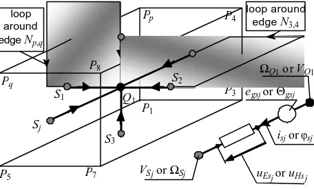
where ksj,N_p,_qis an element of the jth row and Np,qth column of the matrix ks for a graph of a single element.

Pp P4

P8 P7 Pq P5 P3 Sj Si S3 S1 S4 S2 Q1 P1 loop around edge N3,4

loop around edgeNp,q

u_Esj or u_{Hs j} isj orφsj

egsj orΘgsj

V_Sj or Ω_Sj

ΩQ1 or VQ1

An expression for the magnetic potential between nodes for the branch Q1Sj of the facet model may be

derived using the following relationship

∫∫∫

∫∫∫

∫∫∫

e e e V j V j V

jgrad dv 2, dv 2, dv

,

2 w H w T

w (23)

The above expression is a result of the multiplication of the substitution H−T=gradΩ by the jth interpolating function w2,j of a facet element and subsequent

integration. By applying the identity

j j

j 2, 2,

,

2 grad div(w ) divw

w Ω= Ω −Ω (24)

and taking into account that divw_2,j=w₃k_Vj, where kVj

is the jth column of the matrix kV, then for an element of

a single volume, in which w3=w3,1=Ve−1, we find

1 d

d d

grad 1 1

,

2 S Q

V e S j V j j e j e v V S S

v= Ω − Ω =Ω −Ω

Ω

_∫∫

_∫∫∫

∫∫∫

(25)

where ΩS_j is an average value of the potential of the jth facet associated with the node Sj, and ΩQ₁ is an average value of the potential within the volume of the element associated with the node Q1 of the edge graph. Thus the

left hand side of (23) represents the voltage between nodes. When considering the right hand side of (23) the following relationships are helpful

s φ

2

w B

H=ν =ν , T=w1io (26a,b)

Here φs denotes the vector of fluxes passing through

facets, thus branch fluxes, and io the vector of loop

currents ioi,j. Substituting (26) into (23) via (24) yields

gsj n

i Q Q si

Q

Sj−Ω = R i jφ −Θ

Ω

∑

Q1,, 1, =

∫∫∫

µ w w (28a)

∑

1 , ,

n

N jN opq

gsj q p q p i K (28b) and

∫∫∫

K , _, w2, w1, _, d (29)

In the branch equation (27) mutual reluctances

j iQ

Q

Rµ _1,, _1, may be recognised. The magnetic flux in the

ith branch, that is in the branch between nodes Q1 and Si

(Fig. 4), creates a flux in the jth branch between nodes Q1

and Sj. The branch mmfΘgsj may be expressed in terms of

loop (mesh) currents in the loops ‘embracing’ element edges.

In a similar way an expression may be derived for a magnetic voltage between nodes in the branch Q1Sj of the

facet model of an element with an electric field:

gsj n j si Q Q Q

S V Z i e

V _j− =

∑

1 (30)

where dV Z e j i V j i Q

Q1,, 1, =

∫∫∫

∑

1 , ,

) (p n

N jN opq

gsj q p q p K e (31b)

In the branch equation (30) there are mutual impedances of the capacitive type. A current in the ith branch triggers a voltage in the jth branch.

From the relationship (31a) one can deduce expressions for branch resistances for models without displacement currents, as well as branch ‘elastances’ [9], if such currents are present and conduction currents are negligible. The facet model of an element with an electric field has been named the impedance or facet electric (FE) model. The facet model of an element with a magnetic field is known as the reluctance or facet magnetic (FM) model.

The branch parameters of facet models may be established using (19). For example, for a parallelepiped, the following expressions are found

0

, 1 , 1 , = µQ iQ j

R , ZQ_1,i,Q_1,j =0 for i≠ j (32a,b)

2 , 2 , 1 , 1 j e Q Q S V R j j =ν

µ , 2 1 , 2 ) p ( , 1 , 1 j e Q Q S V Z j

j = σ+ ε − (33a,b)

where Sj is the surface area of the ith facet. As a result, a

simplified model of the parallelepiped element is achieved, without couplings between branches, whose parameters are the same as those found using classical approaches, for example a method described in [14].

VII. MODELS OF CONNECTED ELEMENTS

Edge models

Network models of a meshed region are obtained by connecting element models. In the case of an edge model the branches associated with common element edges are connected in parallel. As a result a multi-branch permeance model (EM) is established for a magnetic field or multi-branch conductance-capacitance model (EE) for an electric field.

The vectors ig and φg of branch currents in EE and

branch fluxes in EM may be written in the matrix form

E

g G C u

i =( +p ) , φg=ΛuH (34a,b)

where G, C and Λ are the matrices of branch conductances, capacitances and permeances, respectively; and uE, uH refer to the vectors of potential differences

across elements of the branches of EE or EM. Taking account of (12) allows for these vectors to be written as

g w

E k V e

u = + , u_H =k_wΩ+Θ_g (35a,b)

where V and Ω are vectors of node potentials; eg and Θg

are vectors of branch emfs and mmfs; and kw is a

transposed nodal matrix for the edge graph of the system of connected elements.

In models created using 6-facet elements the branches contain four capacitances and conductances or permeances connected in parallel, such as the branch PiPj

From the above relationships the nodal equations for the permeance network may be established

0

=

+ Tw g

w T

wΛk Ω k ΛΘ

k (36)

and similarly for the conductance-capacitance network

0

= +

+

+ w Tw g

T

w G C k V k G C e

k ( p ) ( p ) (37)

The derived equations correspond to the description of the nodal element method (NEM) using scalar potentials.

Pi

Pj

φgNi,jorigNi,j

ei,j

Electric

ei,j =egNi,j

uk_,j= uH Nk_,j

element 1 element 2

element 3 element 4

Pk uk,j

Magnetic

ei,j=ΘgNi,j uk,j= uHNk_,j

Pq

Fig. 5. Part of an edge model of four elements with details of a branch associated with the edge PiPj

Facet models

When assembling elements for the facet electric (FE) or facet magnetic (FM) model of a meshed region, the branches associated with common facets are connected in series. As a result, a network is established whose nodes are points Qi associated with centres of the volumes, as

shown in Fig. 6. Voltage equations for a branch containing nodes Qi may be written as

s Hs =Rµφ

u , u_Es =Zi_s (38a,b)

where Rµ and Z are the matrices of branch reluctances and branch operational impedances; whereas φs and is are

vectors of branch fluxes and currents. The vectors uHs and uEs may be written in the following form

gs o T V

Hs =k Ω +Θ

u , u_Es=k_VTV_o+e_gs (39a,b)

where Ωo and Vo are vectors of the nodal potentials

associated with centres of elements; Θgs and egs are

vectors of branch mmfs and emfs; finally kV is the matrix

mentioned previously of cuts for the network of connected edge element models.

The vectors φs and is of branch fluxes and currents

are edge vector values of flux and current density, respectively. They may be expressed in terms of edge values of vector potentials, thus in terms of loop fluxes φo

and loop currents io in the loops around the edge of a set

of connected elements. We may write

o s

s φ

φ =k , i_s=k_si_o (40a,b)

where ks is the aforementioned transposed loop matrix of

the facet graph of the connected elements. Fig. 6 depicts part of the facet model of four elements showing a loop ‘embracing’ the edge PiPj.

Pi

Pj

φoNi,jorioNi,j

e1 e2

Magnetic

ek=θk

u1,2=uB1,2

e3

e4

e5

e6

e7

e8

Electric

ek=egsk

u1,2 =uJ1,2

element 1 element 2

element 3 element 4

Q3

Q1 _Q

2

u1,2

Q4

Fig. 6. Part of a facet model of four elements with a loop around the edge PiPj

Loop equations for a reluctance model (SM) of a system with a magnetic field may be established from equations (38), (39) and (40) as

gs T s o s T

sR k φ k Θ

k _µ = (41)

Similarity loop equations for the resistance-elastance model (SE) with an electric field may be written as

gs T s o s T

sZki k e

k = (42)

The loop equations (41) and (42) correspond to edge element formulation (EEM) if vector potentials are used. They may be derived by minimizing the functional with respect to edge values of potentials. Although the approach is known as the edge element method, the branch reluctance and impedance matrices are in fact set up using interpolating functions of the facet element, as shown by equations (28a) and (31a). The functions of the edge element, on the other hand, are helpful when creating the coefficient matrix for the nodal element method, for which the network equivalent is the edge network. In expressions for branch conductances and capacitances as well as for branch permeances of the edge network an absence of classical shape functions of nodal elements may be noticed, as shown by (16) and (18). Notwithstanding, expressions for nodal permeance matrix

w T

w k

k Λ and admittance matrix kT_w(G+pC)k_ware the same as in classical finite element formulation using nodal element. There are, however, differences between the two descriptions when it comes to sources.

VIII. BRANCH AND LOOP SOURC ES

In the models considered the branch mmfs and emfs are described in terms of loop quantities. The branch sources in the facet network (FN) result from loop values in the edge network (EN), whereas branch sources in FN from loop values in EN. Branch mmfs Θb in EN

correspond to loop currents io in FN, e.g. the mmf in the

branch PiPj of the magnetic network of Fig. 5 is equal to

the current in a loop of the electric network that surrounds the edge PiPj (Fig. 6). Branch emfs eb in EN are

found by time differentiation of loop fluxes φo in FN,

hence sources in (36) and (37) may be written as

o g=i

Branch mmfsθ in FM are represented by loop currents ioe in the loops of the edge network, e.g. the branch mmf

in the branch Q1Q3 of the magnetic FN of Fig. 6

corresponds to the loop current in the loop PiPjPqPk of the

electric edge network of Fig. 5. The time derivative of the flux in the loop PiPjPqPk of the EM equals (with negative

sign) the emf in the branch Q1Q3 of the FE. Sources in

(41) and (42) may therefore be written as

oe gs=i

Θ , e_gs=−dφ_oe dt. (44a,b)

where the subscript oe denotes vectors of loop currents and fluxes in the edge networks.

When loop analysis is applied to a network it is not necessary to determine the branch sources, the knowledge of loop sources will suffice. For examp le, when dealing with (41) and (42), it is not essential to establish vectors Θgs and egs of the branch sources, we can focus on

deriving loop sources Θm and em

gs T s

m Θ

Θ =k , em=ksTegs (45a,b).

The loop mmf corresponds to the current passing through a loop of a magnetic network, hence the loop mmfs Θm in the facet network are equivalent to branch

currents ig in the edge network, e.g. the mmf of the loop

shown in Fig 6 (a loop around the edge PiPj) is equal to

the current in the branch PiPj of the electric network of

Fig. 5. The loop emfs, on the other hand, may be found by time differentiating of branch fluxes in the magnetic network passing through loops of the electric network, e.g. loop emfs em in the electric facet network are derived

from fluxes associated with branches of the magnetic edge network as em=−dφg/dt. Thus when solving (41) and

(42) it may be convenient to take into account that

g m gs T

s i

k Θ =Θ = , keTegs =em=−dφg dt (46a,b)

In order to establish branch fluxes φg and branch

currents ig, as well as loop fluxes φoe and loop currents ioe

associated with edge networks, it is not necessary to solve the equations for these networks. Instead, quantities associated with edge networks may be derived from by appropriate transposition of the results for the facet network. The required entries of the transposing matrix K may be found as a product of interpolating functions of the facet and edge elements – as shown by (29). Substitution for K results in the following

o

oe φ

φ =K , i_oe =Ki_o, (47a,b)

s T

g φ

φ =K , i_g =KTi_s. (48a,b)

Moreover, the matrix K may be used to derive currents io and is, as well as fluxes φo and φs, associated

with facet networks, from currents ioe and ig, and also

fluxes φoe and φg , associated with edge networks

oe T

o φ

φ =K , i_o= KTi_oe. (49a,b)

g

s φ

φ =K , i_s= Ki_g. (50a,b)

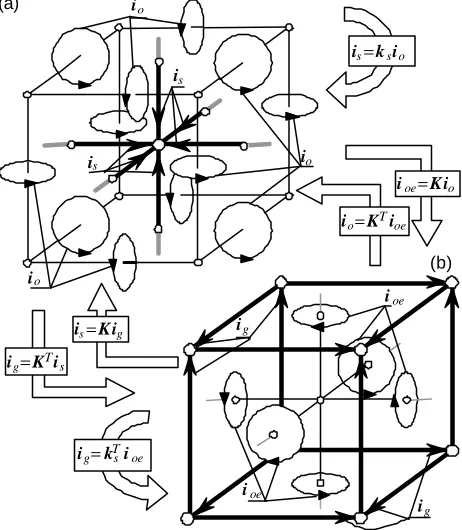
The abovementioned relationships are explained in Fig. 7, where 6-facet elements are considered for which all non-zero entries in K are equal to 1/8.

The loop mmfs in FM may therefore be established

from: (a) branch currents igin EE; (b) loop currents io w

FE; or (c) branch currents is in FE. Equally, to find loop emfs in FE we may use: (a) branch fluxes φg in EM; (b)

loop fluxes φo in FM; or (c) branch fluxes φs in FM. Due

to the bigger variety of descriptions of sources, the facet models are more universal than edge models; this also explains – using the language of circuit theory – why the vector potential formulations are more universal.

(a) io

ioe

ioe

is

ig

ig=kT sioe

io

io

ig

(b)

is

is=ksio

ioe=K io

io=KTioe

ig=KTis

is=Kig

Fig. 7. Transformations of loop and branch currents in networks (a) facet graph, (b) edge graph

IX. COUPLED NETWORK MODELS

The finite element formulations using potentials correspond to equations of magnetic and electric networks coupled via sources.

A–T method

Formulations based on the vector potentials A and T are related to loop equations arising from magnetic and electric facet networks (FM-FE).

Z Rµ

∑

=φ − = + + +

= 8

1 4

3 2 1

d d 8 1

i si m

t e e e e e

Q3 Q4

Q1 Q2

io1,2

e1 e3

e4

e2 is4

is6

is3

is5

is7 is8

is2

is1

∑

= = θ + θ + θ + θ =

Θ 8

1 4 3 2 1

8 1

i si

m i

Q3 Q4

Q1 Q2

φo1,2

θ1 θ3

θ4

θ2 φs4

φs6 φs3

φs5

φs7 φs8

φs2 φs1

FE FM

Fig. 8. Portion of an FM-FE model

from the branch fluxes of the magnetic network we can establish the flux passing through a loop in the electric network. Time derivatives of these fluxes correspond (with negative sign) to loop emfs. The method is particularly suitable for analysis of systems containing thin conductors. In such systems, from the loop equations of the facet electric model the loop equations for circuits containing windings may be established. After taking account of the presence of voltage sources, a system of equations is accomplished containing voltage equations for the windings and FEM equations describing loop fluxes distribution in the magnetic facet network [10].

A–V method

The equations arising from the A–V method, which uses magnetic vector potential and electric scalar potential, contain loop equations of the facet magnetic network and nodal equations of the edge electric network [8, 11]. Coupling exists between the facet magnetic network and edge electric network (FM -EE). Loop mmfs in the magnetic network are derived from branch currents of the electric network, while branch emfs in the electric network are found by differentiating with respect to time of the loop fluxes in the magnetic network (Fig. 9).

Q3 Q4

Q1 Q2

P2

P1

P4 P5

φo1,2 eg1,2

θ1 θ3

θ4

θ2 ig1,2

G+pC Rµ

Θm=θ1+θ2+θ3+θ4=ig1,2

eg1,2=− t d

d _φ

o1,2

FM

EE

Fig. 9. Portion of an FM-EE model

Ω–T method

The method uses a magnetic scalar potential Ω and an electric vector potential T. The resulting equations consist of nodal expressions for the edge magnetic network and loop equations for the facet electric network. The model therefore contains coupled magnetic edge and electric facet networks (EM -FE). The loop emfs are obtained from branch fluxes of the magnetic network, while branch mmfs in the edge network from loop currents of the facet network, as shown in Fig. 10.

Q3 Q4

Q1 Q2

P2

P1

P4 P5

io1,2 θg1,2

e1 e3

e4

e2 φ1,2

Z Λ

em=−e1+e2+e3+e4=−

t d

d _φ 1,2

θg1,2=io1,2

FE

EM

Fig. 10. Portion of a permeance-impedance network

This approach has rarely been used so far. Most commercial codes use two potentials: global and reduced,

while the flow of conduction current is treated as a circuit problem. Moreover, the equivalence between loop currents and the edge values of electric vector potential T is normally overlooked. By taking account of this equivalence, the circuit -field models using the potential O may be treated as a special case of the Ω–T formulation. O–V method

The authors are not aware of publications addressing specifically field analysis using only scalar potentials Ω and V. From the discussion above it follows that the network representation of the equations based on the O–V formulation would involve nodal equations of two edge networks, magnetic and electric. Unfortunately, it is not possible to develop branch mmfs in EE from branch currents in EE, nor branch emfs in EE from branch fluxes in EE. A separate derivation is thus required to establish loop currents and fluxes from branch currents and fluxes, since branch sources in edge networks are defined via loop quantities. The loop values are network equivalents of vector potentials. It may be concluded therefore that the application of the Ω–V formulation would necessitate an additional task of determining the distribution of vector potentials from the knowledge of the scalar potential distribution. For this reason the Ω–V method is considered of little real practical interest and the relevant equations are not elaborated. The equations for the other models are summarised in Table IV.

Table IV. Equations fro the coupled network models

Model Equations

EM-FE Ω−T

0

=

+ Tw g

w T

wΛk Ω k ΛΘ

k , Θ_g=i_o

m o s T

sZk i e

k = , em =−pΛ(kwΩ+Θg)

FM-EE A−V

m o s T

sRµkφ =Θ

k , Θ_m=(G+pC)(k_wV+e_g)

0

= + +

+ w Tw g

T

w G C k V k G C e

k ( p ) ( p ) , e_g=−pφ_o

SM-SE A−T

m o s T

sRµkφ =Θ

k , Θ_m =kT_sKi_o

m o s T

sZk i e

k = , e_m=−kT_sNpφ_o

FE, T

FM, A

m o s T

sZki e

k = , e_m=−pΛi_o (i_o=u_H )

m o s T

sRµk φ =Θ

k , Θ_m=(G+pC)pφ_o (−pφ_o=u_E)

In the bottom row of Table IV, the ‘decoupled’ equations are presented describing loop currents and fluxes in facet models. The relationship for loop fluxes φo

is obtained from equations of the FM-EE model, after imposing the condition kwV=0. The appropriateness of

this condition may be considered by examining the structure of the graph matrices of the facet and edge networks and the properties of the vector Θm on the right

hand side of loop equations for magnetic network in the FM-EE model. This vector is a factor in the system of nodal equations of the network EE. The nodal equations

of EE may be written as kT_wΘ_m =0. The transposed matrix kw is the nodal matrix of the edge network. At the

same time, the matrix ks appearing in the equations of the

are associated with element facets). Consequently,

0 =

T s T wk

k , and thus multiplying both sides of the

equation kT_s R_µk_sφ_o=Θ_m by a transposed matrix kw

leads to kT_wΘ_m=0. Thus the solution satisfying loop equations for FM for the loops around the edges, also satisfies nodal equations for EE, even for kwV=0. If in the

system considered there are no enforced voltages, then when computing the field distribution we may assume that V=0. As a result the task of solving equations of the FM-EE model reduces to a solution of a system of equations describing the loop fluxes φo, i.e. the system

included in the bottom row of Table IV. Hence the electric field distribution may be established by differentation in time of these fluxes, since, as V=0, then from (35b) and (43b) it follows that uE=−pφo. In a similar

way, by substituting Ω=0 in the equations of the Ω–T method, equations describing currents io may be derived

and are included in the bottom row of Table IV. The relationships in that row may be considered as equations of the edge element method for field formulations.

The loop equations for facet networks presented in Table IV for coupled models are ill-posed (underspecified), as the number of independent loops around edges is larger than the number of available independent equations. The loop reluctance and impedance matrices are therefore singular. In early publications about the implementations of EEM the solution algorithms were preceded by procedures to form additional equations to arrive at a well posed system. Several methods were put forward, for example a method utilising the tree of the graph constructed from element edges [13, 15]. In the FM-EE and EM-FE models a well posed system will be accomplished by adding the conditions V=0 and Ω=0. Unfortunately, the known iterative procedures for solving large system of equations are in this case known to be converging rather slowly [2, 17].

Converting EEM equations into a well posed system is not a necessary requirement to obtain a solution. Using an appropriate iterative method, such as ICCG or block relaxation, it is possible to solve these equations, or – to be more precise – find one of the equations satisfying EEM. The iterative process of seeking one of the solutions is converging faster than the process of finding one unique solution of a well posed system [2, 17]. The authors have conducted some tests using the FM -EE model. The comparison concerned the convergence of the well posed system, obtained by adding the condition V=0, and the convergence of an iterative process applied to an underspecified system of equations established using FM and EE models. Despite the fact that incorporating the condition V=0 reduces the number of equations, as there is no need to consider EE, the solution times are longer than for the underspecified system. The number of iterations for solving equations for FM under the condition V=0 was sometimes even two orders of magnitude higher then for the combined FM and EE set.

Using the presented network descriptions it is possible to form models ‘tuned in’ to a particular structure, material properties and imposed conditions. As an example, a system is considered containing thin

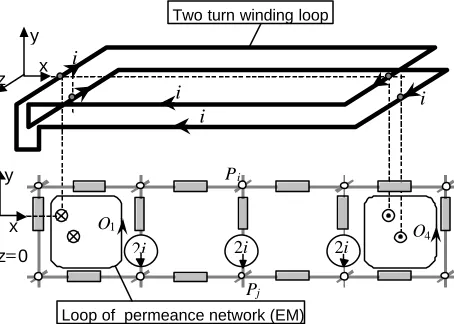
conductors. First, a task of computing magnetic field distribution due to known currents in windings is undertaken, assuming negligible displacement currents. To solve this problem it is convenient to use a permeance model, whose nodal equations correspond to equations NEM using a formulation based on the scalar potential O. In the system under investigation containing thin filamentary conductors, the branch mmfs may be determined from loop currents in the loops of the winding arrangement, after dividing the winding loops into loops around the edges, as described in detail in [10]. Fig. 11 shows an example of a double-turn loop with current and a portion of the permeance network (EM), representing the region within the boundary of the loop. The nodes of the presented portion of the network lie on the plane z=0. The given values of the branch mmfs have been determined by considering the number of cuts of the element edges with the loop surface [10]. From the distribution of these mmfs it follows that, in the portion of the network shown, the non-zero values of mmfs are only in loops O1 and O4, through which the current carrying

conductors pass (Fig. 11). It will also be noted that, thanks to expressing field sources using branch mmfs, it is feasible to employ only one global scalar potential [10]. In the actual algortihm of the nodal method, the branch mmfs are coverted into nodal ‘injections’ of flux (nodal sources). The vector Φ of these injections is described by

the term kT_wΛΘ_g in (36).

x y

z

i

i

i i

2i 2i 2i

x y

z=0

Pi

Pj

O1 _O4

Two turn winding loop

Loop of permeance network (EM)

Fig. 11. A portion of the permerance model of a region with a two-turn coil

It has already been noticed that, in order to describe current distributions in thin conductors supplied from voltage sources, it is most convenient to use the vector potential T. If displacement currents are absent or negligible, then the corresponding to this formulation loop equations of the impedance network may be greatly simplified. By using methods presented in [10], from loop equations of FE, the equations for currents iuo in the

loops of the thin conductors forming the winding may be determined. These equations may be written in a matrix form

zo m T m uo

oi k e u

R = + (51)

where Ro is the loop resistance matrix of the system of

thin conductors; and uzo is the vector of imposed loop

distribution of the winding in the edge element domain [10]. The product of the transposed matrix km and the

vector em (from Table IV) corresponds to the vector of emfs set up by the flux coupled with the winding loops. The matrix equation (51) may be solved together with the equations for model EM or model FM. When defining the sources it should be remembered that io=kmiuo.

The additional ‘external’ circuit currents iuo may be

considered as the edge values of a vector potential T0,

used otherwise in description of multiply connected conductors [4], including analysis of eddy currents in solid conductors with ‘holes’ [1, 5]. After applying EEM to the T formulation, equations representing loop equations of facet network are established. These equations refer to loops with eddy currents around the element edge. Although the number of these loops exceeds the number of independent loops, for a system which is not singly connected it is impossible to set up the system of fundamental loops. It is therefore necessary, for loops around the edges, to supplement the loop equations with equations for additional loops surrounding the ‘holes’. The currents of these loops provide edge values for the potential T0. The authors are

of the opinion that the above explanation, expressed using the language of circuit theory, of the need for the introduction of the additional potential To, is more

convincing than the purely ‘field oriented’ arguments available in the literature.

The network representation of FEM equations is also applicable to the analysis of wave propagation. Fig. 12 shows a network model of a plane electromagnetic wave. The model consists of two coupled networks: facet magnetic and edge electric. Even a short voltage impulse applied to a capacitance in an arbitrary kth branch will create currents even in very distant branches.

Fig.12. Network model of a region with a plane wave, E=1zEz(x), H=1yHy(x)

X. CONCLUSIONS

The article has introduced a notation for the finite element formulation where the description of field quantities is in terms of interpolating functions of an element considered as edge or facet element. In the formulation using functions of an edge element, the edge values of a gradient of a scalar potential are expressed in terms of nodal values. This approach may therefore be called a nodal element method, for brevity, even if the field quantities are described using the functions of the edge element. On the other hand, in the formulation based on the functions of the facet element, the facet values are expressed using edge values of a vector potential, hence it is justifiable to call the method an edge element method.

Equations of the nodal element method for formulations employing scalar potentials correspond to nodal equations of edge networks: electric conductance-capacitance and magnetic permeance. Nodes of the edge network coincide with the element nodes. Equations of the edge element method, on the other hand, for formulations using vector potentials correspond to loop equations of facet networks: magnetic reluctance and electric resistance-elastance. The nodes of the facet network lie in the volume centres of the elements, while loops ‘embrace’ the element edges. The field analysis methods based on scalar potentials represent therefore nodal methods of analysis of electric and magnetic circuits, whereas the field methods employing vector potentials represent the loop approach in circuits.

A particular characteristic of the circuits which serve as analogies to magnetic or electric field systems is the ‘loop’ character of the sources. From the distribution of the current density a loop mmf may be specified, whereas the time variation of the flux density determines the loop emf. For this reason, in the algorithms for the scalar potential method, the routines for solution of FEM are preceded by a procedure forming the sources associated with nodes. In the cases discussed in this article the sources are expressed in terms of edge values of vector potentials, that is in terms of loop currents and fluxes. From these values the branch emfs and mmfs are derived, which – in the process of setting up nodal expressions – are then converted into current and flux injections. As a result, in models of even very non-homogenous regions the sum of the sources associated with nodes is equal to zero and there is no need to use two potentials, global and reduced.

As mentioned already, it is possible to tune the models to cater for particular specific conditions or properties. For example, resistance models can be created of systems containing windings with rod conductors (such as in cage induction motors) where skin effects need to be considered. It is also possible to create models for systems containing displacement currents.

The presented approach is fundamentally different to the classical way of deriving the finite element equations. Probably the most popular derivation relies on a variational principle where the conditions are sought through differentiating the function with respect to nodal, edge or facet values. It important to emphasise, however, that the final equations are identical to those presented in this article. One of the aims of this presentation is to demonstrate that the finite element formulation may be derived entirely from circuit theory without the introduction of the concept of energy functional.

The presented analogies between FEM equations and circuit equations may also be useful to update and enhance the well known and long-in-use network methods of analysis of magnetic circuits, including the permeance networks [6, 16] and reluctance networks [18]. To improve the accuracy of representation of regions of high energy density, the parameters of these models should be established using the expressions presented in this article.

Loop of magnetic network (FM)

Loop of electric network (EE)

Reluctance

Capacitance

x y

z _{Flux φ}

Current i

Details of the solution of large systems of equations resulting from the various networks discussed have not been addressed here. Nevertheless, it was noted that the iterative procedures of solving ill-posed (underspecified) loop equations for facet elements are very efficient. Careful analysis has shown that the loop method does not require the dependent loops to be eliminated.

REFERENCES

[1] Biro O., Preis K., Renhart W., Richter K.R. and Vrisk G., “Performance of different vector potential formulations in solving multiply connected 3 D eddy current problems.” IEEE Trans. on Magnetics. Vol. 26, No. 2, pp.438–441, 1990.

[2] Biro O., Preis K. and Richter K., “On the use of magnetic vector potential in the nodal and edge element analysis of 3d magnetostatic problems,” IEEE Trans. on Magnetics, Vol. 32, No. 3, pp. 651–654, 1996.

[3] Bossavit A., Computational Electromagnetism, Variational Formulations, Complementarity, Edge Elements, San Diego Academic Press, 1998.

[4] Bouissou S. and Piriou F., “Numerical simulation of a power transformer using finite element method coupled to circuit equation,” IEEE Trans. on Magnetics, Vol. 30, No.5, pp. 3224– 3227, 1994.

[5] Bui V. P, Le Floch Y., Meunier G. and Coulomb J.L., “A new three-dimensional (3-D) Scalar Finite Element Method to Compute T0,” IEEE Trans. on Magnetics, Vol. 42, No. 4, pp.

1035–1038, 2006.

[6] Davidson A. and Balchin M. J., “Three dimensional eddy currents calculation using a network method,” IEEE Trans. on Magnetics, Vol. 19, No. 6, pp. 2325–2328, 1983.

[7] Demenko A., Nowak L. and Szelag W., “Reluctance network formed by means of edge element method,” IEEE Trans. on Magnetics, Vol. 34, No. 5, pp. 2485–2488, 1998.

[8] Demenko A., “Three-dimensional eddy current calculation using reluctance-conductance network formed by means of FE method,”

IEEE Trans. on Magnetics. Vol. 36, No. 4, pp.741–745, 2000. [9] Demenko A. and Sykulski J. K., “Network equivalents of nodal

and edge elements in electromagnetics,” IEEE Trans. on Magnetics, Vol. 38, No. 2, pp. 1305–1308, 2002.

[10] Demenko A., “Representation of windings in the 3D finite element description of electromagnetic converters,” IEE Proceedings Science, Measurement and Technology, Vol. 149, No. 5, pp. 186– 189, 2002.

[11] Demenko A. and Sykulski J. K., “Magneto-electric network models in electromagnetism,” COMPEL, Vol., No, pp. , 2006. [12] Dular P., Hody J., Nicolet A., Genon A. and Legros W., “Mixed

finite elements associated with a collection of tetrahedra, hexahedra and prisms,” IEEE Trans. on Magnetics, Vol. 30, No. 5, pp. 2980–2983, 1994.

[13] Golias N.A. and Tsiboukis T.D., “Magnetostatics with edge elements: a numerical investigation in the choice of the tree,”

IEEE Trans. on Magnetics, Vol. 30, No. 5, pp. 2877–2880, 1994. [14] Hammond P. and Sykulski J. K., Engineering Electromagnetism:

Physical Processes and Computation, Oxford University Press, 1994.

[15] Manges J. B. and Cendes Z. J., “A generalised tree-cotree gauge for magnetic field computation,” IEEE Trans. on Magnetics, Vol. 31, No. 3, pp. 1142–1147, 1995.

[16] Ostrovic V., Dynamics of saturated electric machines, Springer-Verlang, Berlin, 1898.

[17] Ren Z., “Influence of R.H.S. an the convergence behaviour of the curl-curl equation,” IEEE Trans. on Magnetics, Vol. 32, No. 3, pp. 655–658, 1996.

[18] Sykulski J. K., Stoll J., Sikora R., Pawluk K., Turowski J. and Zakrzewski K., Computational Magnetics, London, Chapman & Hall, 1995.

Andrzej Demenko [email protected]

Jan K. Sykulski [email protected]