IMAGING TECHNIQUES
Thesis by Jigang Wu
In Partial Fulfillment of the Requirements for the Degree of
Doctor of Philosophy
CALIFORNIA INSTITUTE OF TECHNOLOGY
Pasadena, California 2009
© 2009
ACKNOWLEDGEMENTS
First I would like to thank my advisor, Professor Changhuei Yang, for giving me the opportunity to work in the interesting area of biomedical optical imaging. He was constantly a great source of ideas when I encountered problems in my research, and most of the ideas turned out to be very helpful. And most importantly, I was always motivated by his passion for engineering and science. Without his support, it would be impossible for me to successfully finish my many exciting research projects.
I am grateful to Professors Scott Fraser, Yu-Chong Tai, P. P. Vaidyanathan, and Amnon Yariv for being my thesis committee and also my candidacy committee. They were always available when I need help.
I have enjoyed working in the friendly and creative research group of biophotonics at Caltech. Numerous discussions with lab colleagues during working hours and social hours frequently gave me inspiration and ideas. Dr. Zahid Yaqoob helped me with many experiments, including optical coherence tomography and the G1G2 phase imaging techniques, and I benefited a lot from our discussions. Dr. Xin Heng, Xiquan Cui, and Lap Man Lee helped me learn microfabrication, microfluidics, and gave many useful suggestions for my research projects. I have spent lots of time with Dr. Xin Heng talking about simple or crazy ideas on scientific research. Xiquan Cui has spent his precious time helping me with fabrication of OFM apertures using FIB. Lap Man Lee has helped me with fabrication of microfluidic channels. I also thank other group members: Emily McDowell, Jian Ren, Guoan Zheng, Shuo Pang, and Ying Min Wang for their friendship and numerous technical discussions during these years.
Finally, I would like to thank my parents and siblings for their love and support during my life. It is hard to imagine that I can have the perseverance to finish my graduate study without their support.
ABSTRACT
Coherence domain optical imaging techniques have been developing quickly in the past few decades after the invention of laser. In this thesis, I will report the imaging methods that constitute my research projects during these years of graduate studies, including paired-angle-rotation scanning (PARS) forward-imaging probe for optical coherence tomography (OCT), full-field phase imaging technique based on harmonically matched diffraction grating (G1G2 grating), and Fresnel zone plate (FZP) based optifluidic microscopy (OFM). Compared with conventional optical microscopy, the coherence domain optical imaging has many advantages and greatly extends the application of imaging techniques.
OCT, based on low-coherence interferometry, is a high-resolution imaging technique that has been successfully applied to many biomedical applications. The development of various probes for OCT further made this technique applicable to endoscopic imaging. In the project of PARS-OCT probe, I have developed a forward-imaging probe based on two rotating angle-cut GRIN lenses. The diameter of the first prototype PARS-OCT probe that I made is 1.65 mm. My colleagues further built a probe with diameter of 0.82 mm. To our knowledge, this is the smallest forward-imaging probe that has been reported. The first prototype probe was characterized and successfully used to acquire OCT images of a Xenopus laevis tadpole.
OFM is a novel high-resolution and low-cost chip-level microscope developed by our group several years ago. Combining the unique imaging concept and microfluidic techniques, OFM system can be potentially useful to many biomedical applications, such as cytometry, blood parasite diagnosis, and water quality inspection. In the project of FZP-OFM, I applied the FZP to project the OFM aperture array onto an imaging sensor for OFM imaging. In this way, the sensor and the aperture array can be separated and will be useful for some situations. To demonstrate its capability, the FZP-OFM system was used to acquire OFM images of the protist Euglena gracilis.
TABLE OF CONTENTS
Acknowledgements ... iv
Abstract ... vi
Table of Contents...viii
List of Illustrations and Tables ... ix
Nomenclature...xii
Chapter I: Introduction ... 1
Overview of Optical Biomedical Imaging Methods ... 1
Coherence Domain Optical Imaging Methods ... 3
Structure of the Thesis... 6
References... 6
Chapter II: Optical Coherence Tomography Forward-Imaging Probe ... 10
Principle of Optical Coherence Tomography ... 11
Experimental Setup of Swept-Source Based OCT System... 16
Paired-Angle-Rotation Scanning (PARS) Forward-Imaging Probe... 19
References... 30
Appendix A: Derivation of Equation (2.14) ... 32
Chapter III: Full-Field Phase Imaging Principle with Harmonically Matched Diffraction Grating (G1G2 Grating)... 35
Overview of Related Phase-Imaging Techniques ... 36
Harmonically Matched Diffraction Grating ... 38
Experimental Setups... 44
Proof-of-Principle Experiments ... 49
References... 52
Chapter IV: Phase Imaging of Biological Samples with G1G2 Interferometry ... 53
Improved Experimental Setup for Imaging Biological Samples ... 53
Improved Data Processing ... 59
Phase Noise Analysis ... 66
Application in Phase Imaging of Biological Samples... 70
References... 73
Chapter V: Fresnel Zone Plate Based Projection in Optofluidic Microscopy . 74 Principles of Optofluidic Microscopy (OFM) ... 74
Characteristics of Fresnel Zone Plate and Its Fabrication... 79
Experimental Setup ... 84
Application in OFM Imaging... 92
References... 95
Chapter VI: Conclusion ... 97
Summary... 97
LIST OF ILLUSTRATIONS AND TABLES
Illustrations Page
2.1. Illustration of time-domain OCT system... 11
2.2. Principle of spectral-domain OCT... 13
2.3. Experimental setup of swept-source based OCT ... 17
2.4. Schematic of trigger generation module... 18
2.5. Flow chart of program for the PARS-OCT probe imaging ... 19
2.6. Schematic of the PARS-OCT probe ... 20
2.7. Calculated B-scan mode profile... 22
2.8. Paraxial ray tracing of GRIN lens... 23
2.9. Calculated and measured exit beam polar angle ... 24
2.10. Scanning modes of the needle probe ... 24
2.11. The variation of the output power... 25
2.12. Actuation system and the PARS-OCT probe ... 25
2.13. Schematic of measuring the focus size of the exit beam... 27
2.14. OCT image of the heart of a stage 54 Xenopus laevis... 28
2.15. OCT images of the gill pockets of a stage 54 Xenopus laevis... 29
2.16. Definition of some parameters of the forward-scanning probe ... 30
2A.1. Refraction at the angled face of the second GRIN lens ... 32
3.1. Schematic of digital holography ... 36
3.2. Interferometer based on 3 × 3 fiber coupler ... 37
3.3. Interferometer based on common beamsplitter and single grating... 39
3.4. Additional phase shifts in a single grating based interferometer ... 41
3.5. Additional phase shifts in a G1G2 grating based interferometer... 42
3.6. Experimental setup for recording the G1G2 grating ... 45
3.7. The Mach-Zehnder interferometer setup for phase imaging ... 47
3.9. Nontrivial phase shift of interference signals of the G1G2 grating .... 48
3.10. Phase image of double bars fabricated on an ITO glass ... 49
3.11. Observing the diffusion process in a microfluidic channel... 51
4.1. Geometric aberration induced by the grating ... 55
4.2. “Stretch” and “compression” distortion caused by the grating... 56
4.3. Calculation of the “stretch” and “compression” distortion ... 58
4.4. Experimental setup for phase imaging ... 59
4.5. Elliptic fitting of the time series of signals from two pixels ... 62
4.6. Compare unwrap algorithms... 65
4.7. Schematic of the phase noise assessment ... 67
4.8. Measurement of the temporal phase stability ... 68
4.9. Images of “CIT” logo by our imaging system... 70
4.10. Images of onion skin cells... 71
4.11. Phase images of a moving amoeba proteus at four different times .. 72
5.1. Two possible arrangement of the aperture array direction... 75
5.2. Schematic for measuring the PSF of the aperture ... 78
5.3. Schematic of the Fresnel zone plate... 80
5.4. Chrome mask of the Fresnel zone plate... 82
5.5. Fabrication procedure of our FZP... 82
5.6. Images of resolution bars acquired by direct imaging of the FZP ... 84
5.7. Imaging scheme of the FZP ... 85
5.8. Signals of α, β-hole ... 87
5.9. Transmitted signal of the apertures... 87
5.10. Inlet of the microfluidic channel... 88
5.11. Illumination for the FZP-OFM and the microscope module ... 89
5.12. Experiment to characterize the imaging quality of the FZP ... 91
5.13. Images of Euglena gracilis by FZP-OFM and microscope ... 93
5.15. An example of OFM image of a rotating microsphere ... 94
NOMENCLATURE
FZP. Fresnel zone plate.
G1G2 grating. Harmonically matched diffraction grating.
G1G2 interferometry. Interferometry based on harmonically matched diffraction grating. OCT. Optical coherence tomography.
OFM. Optofluidic microscopy.
C h a p t e r I
INTRODUCTION
The area of optical imaging has a long history and was revolutionized since the invention of laser. The recent decades have witnessed a rapid development of various optical biomedical imaging methods, and many of them were based on coherence domain optical techniques. Compared with other biomedical imaging techniques such as x-ray imaging, ultrasound imaging, or magnetic resonance imaging (MRI), optical biomedical imaging methods usually have the advantages of being unharmful, high resolution, and high sensitivity, etc. [1]. In this chapter, I will introduce some important optical biomedical imaging techniques, and then focus on the advantages of the imaging methods from my research in the thesis.
Overview of Optical Biomedical Imaging Methods
Generally, the purpose of optical biomedical imaging is to provide images with contrast between different microscopic structures of the sample for biological studies or medical diagnosis. Current optical biomedical imaging methods include conventional microscopy and its adaptations, fluorescence and nonlinear imaging methods, near-field microscopy, and interferometric methods, etc. Some of these techniques can also be combined together for some specific applications. Furthermore, many techniques can be miniaturized to provide endoscopic imaging of biological samples.
be transmission or reflection based, bright-field or dark-field, and can be adapted to provide more functionality. For example, phase contrast microscopy [2, 3] and differential interference const (DIC) microscopy [4] were developed to provide phase information of the sample where the intensity information is hard to be observed, e.g., transparent sample.
In addition to full-field microscopy, scanning microscopy was also developed. One of the most important examples is the confocal scanning microscopy, where a confocal aperture is used as a spatial filter to reject the light from the out-of-focus region [5]. Using the scanning method and the confocal aperture, the technique can acquire images with large field of view and high sensitivity. Besides direct imaging of the sample, the confocal microscope is also very important for other imaging techniques including fluorescence and nonlinear methods.
In fluorescence microscopy [6], the fluorescence light emitted by fluorophores is separated from the excitation light by optical filter and collected for imaging. Fluorescence techniques are widely used for many biomedical studies as they can be used to identify submicroscopic structures and even a single molecule. Super resolution (<50 nm) techniques, such as stochastic optical reconstruction microscopy (STORM) [7] or photoactivated localization microscopy (PALM) [8], have been developed based on sequential imaging of single fluorophore molecules. In addition to the simple fluorescence microscopy, fluorescence phenomenon is also used in many other techniques, such as fluorescence resonance energy transfer (FRET) [9] imaging or fluorescence lifetime imaging microscopy (FLIM) [10]. Nonlinear imaging techniques, such as second-harmonic microscopy [11] and coherent anti-Stokes Raman scattering (CARS) microscopy [12], also provide images with very high sensitivity.
The above imaging methods are based on far-field optical imaging, and the resolution is generally limited by diffraction effect. In order to overcome the diffraction limit, near-field
techniques are developed to achieve imaging with higher resolution (≤100 nm). Near-field
region of the sample surface and illuminate a small region of the sample. The signal is collected while the probe is scanning. Because of the near-field property, the light is localized and thus much better resolution can be achieved, compared with the far-field techniques.
In recent years, many coherence domain optical imaging methods [14] are developed. Compared with other optical imaging methods, coherence domain methods have many advantages and greatly extend the application of optical techniques. Because of the broad varieties of various methods, I am not going to give a comprehensive review of all the coherence domain techniques. Instead, I will focus on the imaging methods of my research in the thesis in the next section.
Coherence Domain Optical Imaging Methods
Most of the coherence domain optical imaging methods fall into two categories: (1) interferometer-based techniques, e.g., holography, and optical coherence tomography (OCT) [15]. (2) scattering or laser speckle based techniques, e.g., diffusing wave spectroscopy (DWS) [16], and laser speckle imaging [17].
Optical coherence tomography is an important biomedical imaging technique being extensively developed since the early 1990s. Compared with other imaging techniques, OCT has the following important advantages: (1) The laser source is usually infrared, thus is not harmful to human tissue. (2) The system is based on low-coherence interferometer and the resolution is limited by the coherence length of the laser, thus high-resolution (~1–
10 μm) can be achieved. (3) The system can be fiber based, thus can be easily made
compact and low cost. (4) The data reconstruction is relatively easy, thus real-time imaging can be achieved. Because of these and other numerous advantages, OCT has been established as an important tool in biomedical imaging area. The application of OCT in ophthalmology is now very common in hospitals. OCT has also been used in dermatology [18] and early cancer detection [19].
autocorrelation of the light field is measured directly, which corresponds to the depth-scanning signal of the sample. In contrast, in spectral-domain OCT, the autocorrelation is calculated by the Fourier transform of the power spectral signal that is measured directly. During the early years of OCT, time-domain implementation was prevailingly popular because of its relatively simple principle and implementation that can be easily understood. However, spectral-domain OCT gets more popular after the researchers discovered that spectral-domain OCT has a major advantage over the time-domain embodiment –– significant sensitivity improvement for the same laser power [20, 21]. Spectral-domain OCT can be implemented by setting up a spectrometer to detect the interference signal [22] or using a swept source to scan the frequency of the laser [23]. In my study, a swept-source based OCT was used. Its principle will be explained in chapter 2.
Besides the basic implementation of OCT, this technique has been greatly expanded for different applications. Several examples are (1) functional OCT –– the use of OCT signal to study information from the sample other than acquiring simple structure image, e.g., polarization-sensitive OCT [24], optical Doppler tomography [25], and spectroscopic OCT [26]; (2) optical coherence microscopy [27] –– the advantages of OCT and confocal microscopy can be combined to further increase the sensitivity of microscopy; (3) parallel or full-field OCT [28, 29] –– remove the scanning necessity of OCT so that the imaging speed can be greatly improved; (4) endoscopic OCT [30] –– implementation of endoscopic probe for OCT to extend the application range of the technique. One project of my thesis is to develop an endoscopic OCT probe for forward-imaging application [31].
interferograms with different phase shifts are acquired sequentially and combined to calculate the quantitative phase. (3) Digital holography [35] or Hilbert phase microscopy [36] –– where the phase image are generated from interferogram encoded with high-frequency spatial fringes. (4) Polarization quadrature microscopy [37] –– where a polarization based quadrature interferometer was used to generate phase image.
These phase imaging techniques generally require some form of nontrivial encoding (in time, space, or polarization) for phase extraction. The encoding process usually entails a more complicated experimental setup, computationally intensive postprocessing, or some sacrifice in the imaging field of view. To overcome some of these problems, our group has developed a novel full-field phase imaging technique based on the substitution of a conventional beamsplitter with a harmonically matched grating pair (G1G2 grating) [38– 40]. This is one of the projects in my thesis and will be explained in detail in chapter 3 and 4.
In this research project, we noted that a FZP can be used to project the image of the aperture array onto the imaging sensor to acquire OFM images, which is not affected by the aberration of the FZP. In this way, the aperture array and the imaging sensor can be separated, and we can still have a compact microscope thanks to the small size of the fabricated FZP. The details of this project will be explained in chapter 5.
Structure of the Thesis
In chapter 2, I will explain the principles of OCT and the swept-source OCT setup for my experiment, and the details of the paired-angle-rotation scanning (PARS) forward-imaging probe, including theoretical calculation, simulation, and experimental verifications. In chapter 3, I will first overview the digital holography technique and the 3 × 3 fiber coupler based interferometer, then introduce the concept of harmonically matched diffraction grating and the G1G2 interferometry, and then show the experimental setup for acquiring phase image and the results of proof-of-principle experiments. In chapter 4, I will explain the improved G1G2 interferometer, including improvement in experimental setup and data processing algorithm. Next I will give an analysis of the associated phase noise in the system. Then I will show the imaging results of biological samples by the G1G2 interferometer. In chapter 5, I will explain the principles of the OFM and the characteristics of the FZP used in our experiment for projection in OFM, and then show the experimental setup and imaging results. Finally in chapter 6, I will conclude my thesis with a summary of my research projects and some possible future studies.
References
1. P. N. Prasad, Introduction to Biophotonics (John Wiley & Sons, 2003).
2. F. Zernike, “Phase contrast, a new method for the microscopic observation of
transparent objects,” Physica 9, 686-698 (1942).
3. F. Zernike, “Phase contrast, a new method for the microscopic observation of
transparent objects Part II,” Physica 9, 974-986 (1942).
4. R. D. Allen, G. B. David, and G. Nomarski, “The Zeiss-Nomarski differential
interference equipment for transmitted light microscopy,” Zeitschrift für
Wissenschaftliche Mikroskopie und Mickroskopische Technik 69, 193-221 (1969).
5. T. Wilson, Editor, Confocal Microscopy (Academic Press, 1990).
6. F. W. D. Rost, Fluorescence microscopy, vol. 1 (Cambridge University Press, 1992).
7. M. Bates, B. Huang, G. T. Dempsey, X. Zhuang, “Multicolor super-resolution
8. E. Betzig, G. H. Patterson, R. Sougrat, O. W. Lindwasser, S. Olenych, J. S. Bonifacino, M. W. Davidson, J. Lippincott-Schwartz, H. F. Hess, “Imaging
intracellular fluorescent proteins at nanometer resolution,” Science 313, 1642-1645
(2006).
9. G. W. Gordon, G. Berry, X. H. Liang, B. Levine, and B. Herman, “Quantitative
fluorescence resonance energy transfer measurements using fluorescence
microscopy,” Biophysical Journal 74, 2702-2713 (1998).
10. P. I. H. Bastiaens, and A. Squire, “Fluorescence lifetime imaging microscopy: Spatial
resolution of biochemical processes in the cell,” Trends in Cell Biology 9, 48-52
(1999).
11. L. Moreaux, O. Sandre, and J. Mertz, “Membrane imaging by second-harmonic
generation microscopy,” Journal of the Optical Society of America B 17, 1685-1694
(2000).
12. J. X. Cheng, and X. S. Xie, “Coherent anti-Stokes Raman scattering microscopy:
Instrumentation, theory, and applications,” Journal of Physical Chemistry B 108,
827-840 (2004).
13. R. C. Dunn, “Near-field scanning optical microscopy,” Chemical Reviews 99,
2891-2827 (1999).
14. V. V. Tuchin, Editor, Handbook of coherent domain optical methods, vol. 1, 2
(Kluwer Academic Publishers, 2004).
15. D. Huang, E. A. Swanson, C. P. Lin, J. S. Schuman, W. G. Stinson, W. Chang, M. R.
Hee, T. Flotte, K. Gregory, C. A. Puliafito, and J. G. Fujimoto, “Optical coherence
tomography,” Science 254, 1178-1181 (1991).
16. D. J. Pine, D. A. Weitz, P. M. Chaikin, and E. Herbolzheimer, “Diffusing-wave
spectroscopy,” Physical Review Letters 60, 1134-1137 (1988).
17. J. D. Briers, “Laser Doppler, speckle and related techniques for blood perfusion
mapping and imaging,” Physiological measurement 22, R35-R66 (2001).
18. M. Mogensen, H. A. Morsy, L. Thrane, and G. B. E. Jemec, “Morphology and
epidermal thickness of normal skin imaged by optical coherence tomography,”
Dermatology 217, 14-20 (2008).
19. S. A. Boppart, W. Luo, D. L. Marks, and K. W. Singletary, “Optical coherence
tomography: feasibility for basic research and image-guided surgery of breast cancer,”
Breast Cancer Research and Treatment 84, 85-97 (2004).
20. M. A. Choma, M. V. Sarunic, C. Yang, and J. A. Izatt, “Sensitivity advantage of
swept source and Fourier domain optical coherence tomography,” Optics Express 11,
2183-2189 (2003).
21. R. Leitgeb, C. K. Hitzenberger, and A. F. Fercher, “Performance of Fourier domain
vs. time domain optical coherence tomography,” Optics Express 11, 889-894 (2003).
22. M. Wojtkowski, R. Leitgeb, A. Kowalczyk, T. Bajraszewski, and A. F. Fercher, “In
vivo human retinal imaging by Fourier domain optical coherence tomography,”
Journal of Biomedical Optics 7, 457-463 (2002).
23. S. R. Chinn, E. A. Swanson, and J. G. Fujimoto, “Optical coherence tomography
using a frequency-tunable optical source,” Optics Letters 22, 340-342 (1997).
24. J. F. de Boer, S. M. Srinivas, B. H. Park, T. H. Pham, Z. Chen, T. E. Milner, and J. S.
tissues,” IEEE Journal of Selected Topics in Quantum Electronics 5, 1200-1204
(1999).
25. Y. Zhao, Z. Chen, C. Saxer, S. Xiang, J. F. de Boer, and J. S. Nelson, “Phase-resolved
optical coherence tomography and optical Doppler tomography for imaging blood flow in human skin with fast scanning speed and high velocity sensitivity,” Optics Letters 25, 114-116 (2000).
26. U. Morgner, W. Drexler, F. X. Kartner, X. D. Li, C. Pitris, E. P. Ippen, and J. G.
Fujimoto, “Spectroscopic optical coherence tomography,” Optics Letters 25, 111-113
(2000).
27. J. A. Izatt, M. R. Hee, G. M. Owen, E. A. Swanson, and J. G. Fujimoto, “Optical coherence microscopy in scattering media,” Optics Letters 19, 590-592 (1994).
28. M. Ducros, M. Laubscher, B. Karamata, S. Bourquin, T. Lasser, and R. P. Salathe,
“Parallel optical coherence tomography in scattering samples using a two-dimentional
smart-pixel detector array,” Optics Communications 202, 29-35 (2002).
29. L. Vabre, A. Dubois, and A. C. Boccara, “Thernal-light full-field optical coherence
tomography,” Optics Letters 27, 530-532 (2002).
30. Z. Yaqoob, J. Wu, E. J. McDowell, X. Heng, and C. Yang, “Methods and application
areas of endoscopic optical coherence tomography,” Journal of Biomedical Optics 11,
063001 (2006).
31. J. Wu, M. Conry, C. Gu, F. Wang, Z. Yaqoob, and C. Yang, “Paired-angle-rotation
scanning optical coherence tomography forward-imaging probe,” Optics Letters 31,
1265-1267 (2006).
32. A. Barty, K. A. Nugent, D. Paganin, and A. Roberts, “Quantitative optical phase
microscopy,” Optics Letters 23, 817-819 (1998).
33. M. V. Sarunic, S. Weinberg, and J. A. Izatt, “Full-field swept-source phase
microscopy,” Optics Letters 31, 1462-1464 (2006).
34. K. Creath, “Phase-measurement interferometry techniques,” Progress in Optics 26,
349-393 (1988).
35. P. Marquet, B. Rappaz, P. J. Magistretti, E. Cuche, Y. Emery, T. Colomb, and C.
Depeursinge, “Digital holographic microscopy: a noninvasive contrast imaging technique allowing quantitative visualization of living cells with subwavelength axial accuracy,” Optics Letters 30, 467-470 (2005).
36. T. Ikeda, G. Popescu, R. R. Dasari, and M. S. Feld, “Hilbert phase microscopy for
investigating fast dynamics in transparent systems,” Optics Letters 30, 1165-1167
(2005).
37. D. O. Hogenboom, C. A. DiMarzio, T. J. Gaudette, A. J. Devaney, and S. C.
Lindberg, “Three-dimensional images generated by quadrature interferometry,” Optics Letters 23, 783-785 (1998).
38. Z. Yaqoob, J. Wu, X. Cui, X. Heng, and C. Yang, “Harmonically-related diffraction
gratings-based interferometer for quadrature phase measurements,” Optics Express 14,
8127-8137 (2006).
39. J. Wu, Z. Yaqoob, X. Heng, L. M. Lee, X. Cui, and C. Yang, “Full field phase
40. J. Wu, Z. Yaqoob, X. Heng, X. Cui, and C. Yang, “Harmonically matched grating-based full-field quantitative high-resolution phase microscope for observing dynamics of transparent biological samples,” Optics Express 15, 18141-18155 (2007).
41. J. Wu, X. Cui, L. M. Lee, and C. Yang, “The application of Fresnel zone plate based
projection in optofluidic microscopy,” Optics Express 16, 15595-15602 (2008).
42. X. Heng, D. Erickson, L. R. Baugh, Z. Yaqoob, P. W. Sternberg, D. Psaltis, and C.
C h a p t e r I I
OPTICAL COHERENCE TOMOGRAPHY FORWARD-IMAGING PROBE
In this chapter I will first explain the principle of OCT, including time-domain systems and spectral-domain systems, and the swept-source OCT system setup that was used with the probe, and then show the scanning mechanism of the PARS probe and the characteristics of the first-version probe. Finally, we will show some OCT images acquired by the PARS-OCT probe to demonstrate its capability.
Principle of Optical Coherence Tomography
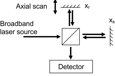
[image:23.612.225.423.310.440.2]OCT is in principle a low-coherence interferometer, and can be implemented as time-domain or spectral-time-domain systems. The principle of time-time-domain system is illustrated in Fig. 2.1. In the following discussion, we shall ignore the polarization and dispersion effect.
Figure 2.1. Illustration of time-domain OCT system.
In the system, a broadband laser source is split into two arms, called reference arm and sample arm. In the experiment, the sample arm will illuminate and collect light from the sample, and the reference arm will provide a delayed reference signal. Finally the light from the sample arm and the reference arm will interfere and the resulting OCT signal is detected by the detector. In the time-domain OCT system, usually the reference arm is scanned and the OCT signal P, omitting the DC signal, can be written as
)} ( { )
) (
2 ( ) ( )
( * ω
S FT c
x x t E t E x
x
P r s
s
r =
− +
=
− , (2.1)
Broadband laser source
Detector xr
where E(t) is the electric field of the laser source, t is time, xr and xs are the optical path
lengths of the reference and sample arm, and c is the speed of light. Here we suppose the
light field is a wide-sense stationary random process. The interference signal is actually the autocorrelation of the light field and depends only on the delay of the two arms, xr−xs, and,
according to the Wiener-Khintchine theorem, is the Fourier transform of power spectrum of
the laser. In the equation, FT{} denotes the Fourier transform and S(ω) is the power
spectrum of the laser. Thus, for a broadband source, the OCT signal only has significant value when xr-xs is smaller than the coherence length. Suppose the sample is a mirror, then
the position of the mirror can be measured precisely. And if the sample has layered structures, the positions of the different layers can also be measured. Thus the scanning of the reference arm will provide an axial scan (A-scan) into the sample. And a 2D image of sample can be obtained if we perform multiple A-scans (called a B-scan, as similar to ultrasound imaging). According to the above discussion, we can see that the transverse resolution is limited by the sample arm optics as in conventional microscope. The axial resolution of OCT is limited by the coherence length of the laser source and inversely proportional to the bandwidth of the source. For a source with spectrum of Gaussian profile, the axial resolution can be expressed as [12]
λ λ π Δ =
Δx 2ln2 2 , (2.2)
where λ is the center wavelength of the laser and Δλ is the bandwidth of the spectrum.
Thus the axial resolution is inversely proportional to the laser bandwidth, and OCT usually requires broadband laser to achieve high axial resolution.
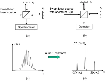
that the interference signal is obtained by the spectrometer or by scanning the wavenumber k of the laser source instead of scanning the delay of reference beam.
Figure 2.2. Principle of spectral-domain OCT. (a) Spectrometer based OCT; (b) swept-source based OCT; (c) detected signal P(k) as the wavenumber k is sweeping; (c) Fourier transform of the detected signal P(k) gives the position information.
Suppose the laser source has a spectrum S(k). The optical power P(k), detected by the
spectrometer at different k or the detector when k is sweeping, can be written as
)) (
2 cos( ) ( ) ( 2 ) ( ) ( )
(k Sr k Ss k Sr k Ss k k xr xs
P = + + − , (2.3)
Swept laser source with spectrum S(k)
Detector xr
xs
Fourier Transform
k -2(xr-xs) x
) (k
P FT{P(k)}
(a)
(c) (d) 2(xr-xs)
Broadband laser source
Spectrometer xr
xs
where Sr(k) and Ss(k) is the power returned from the reference mirror and the sample
mirror. A typical interferogram is shown in Fig. 2.2(c). The position information, xr-xs, can
then be obtained by Fourier transform of P(k):
))], ( 2 ( )) ( 2 ( [ 2 1 * } ) ( ) ( { 2 )} ( { )} ( { )} ( { s r s r s r s r x x x x x x k S k S FT k S FT k S FT k P FT − − + − + + + = δ δ (2.4)
where * denotes convolution. Suppose the reference arm and the sample arm do not change the light spectrum, then we can write Sr(k)=RrS(k) and Ss(k)=RsS(k), where Rr and Rs are
reflectance of reference and sample arm, respectively. Thus, equation (2.4) can be written as ))], ( 2 ( )) ( 2 ( [ * )} ( { )} ( { ) ( )} ( { s r s r s r s r x x x x x x k S FT R R k S FT R R k P FT − − + − + + + = δ δ (2.5)
Thus, FT{P(k)} provides the axial position information of the sample, as shown in Fig.
2.2(d). From the equation we note that the width of the interference peaks are determined by the Fourier transform of the laser spectrum S(k), similar as the time-domain case. Thus
the resolution of spectral-domain OCT is limited by the coherence length of the laser source, just as in time-domain OCT. However, there is an important difference between spectral-domain and time-domain OCT. From the equation and the figure, we note that for the same sample position xs, there will be two peaks in the Fourier transformed axial scan
line. This phenomenon are called complex conjugate artifact [13] of spectral-domain OCT. The artifact prevents the spectral-domain OCT from resolving the positive path length difference from the negative one. Researchers have developed many methods [13, 14] to resolve the artifact problem and expand the scan range of OCT. In our experiment, the sample is positioned only in half of the space and we do not need to resolve the artifact problem.
Fourier transform will be periodic. For systems without resolving the complex conjugate artifact, the effective axial scan range can be written as [15]
k x
δ π 2
max = , (2.6)
where δk is the spectral resolution of the sampling in k space.
Another important difference between the spectral-domain and time-domain OCT is the phenomenon of SNR falloff as the optical path length difference between the reference arm and sample arm gets larger [15, 16]. This is due to the finite linewidth of the swept source in swept-source based system, and the finite pixel width of the array detector in the spectrometer based system. In practice, this SNR falloff is less in swept-source system (~10 dB for the whole scan range in our swept-source system) than in spectrometer based system (~20 dB for the whole scan range in our spectrometer based system) because of the narrow linewidth of swept source.
Usually in an OCT system, the resolution and the sensitivity can be seriously affected by dispersion mismatch between reference arm and sample arm [12]. In time-domain OCT, we will have to make sure the dispersions of the two arms are matched for optimal results, sometimes by inserting additional dispersion materials [17]. In spectral-domain OCT, however, the dispersion compensation can be implemented by software algorithm [18]. This is another important advantage of spectral-domain OCT over time-domain OCT. Nevertheless, in our swept-source OCT system, as the fiber SMF-28 (Corning) almost has no dispersion around the working wavelength of 1300 nm, we do not need to do dispersion compensation.
One of the most important reasons that the spectral-domain OCT become popular is its SNR advantages over the time-domain OCT. Suppose the spectral-domain OCT acquire
signals in M evenly spaced k, then the SNR improvement over the time-domain system that
has the same laser power and same A-line scan rate is roughly M/2 [15], if shot noise
the corresponding position points in an A-scan is M/2, considering the complex
conjugate artifact. Suppose the spectral-domain OCT and the time-domain OCT has the same acquisition time t for an A-scan, then the time for acquiring signal for one point is
Spectral-domain OCT: tSDOCT =t,
Time-domain OCT:
2 /
M t tTDOCT = ,
(2.7)
(2.8)
This is because in spectral-domain OCT, the whole A-scan line is always illuminated during t. Instead, in time-domain OCT, the signal for a position point in A-scan line is only
collected when the reference beam scan to the equal-pathlength position. We know that the SNR of the system is directly proportional to the acquisition time, and thus the SNR of the
spectral-domain OCT will be M/2 times higher than the time-domain OCT.
Experimental Setup of Swept-Source Based OCT System
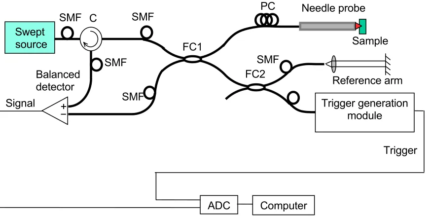
Figure 2.3. Experimental setup of swept-source based OCT. SMF: single-mode fiber; C: circulator; PC: polarization controller: ADC: analog-to-digital converter; FC1 and FC2: fiber coupler 1 and 2.
The two interference signals detected by the balanced detector can be written as, similar to equation (2.3): )) ( 2 cos( ) ( ) ( 2 ) ( ) ( ) (
1 k Sr k Ss k Sr k Ss k k xr xs
P = + + − ,
)) ( 2 cos( ) ( ) ( 2 ) ( ) ( ) (
2 k Sr k Ss k Sr k Ss k k xr xs
P = + − − .
(2.9)
(2.10)
They were 180o out of phase, and the balanced detector detected the difference of the two
signals, which was
)) ( 2 cos( ) ( ) ( 4 ) ( ) ( )
(k P1 k P2 k Sr k Ss k k xr xs
P = − = − . (2.11)
In this way, the DC terms of the interference signals were canceled and the interference term was doubled. Furthermore, the noise associated with the DC term, such as the power fluctuation, will be canceled. Thus the balanced detection can significantly improve the signal-to-noise ratio (SNR) of the system. Note that the beat noise, which is a component of the excess noise, still cannot be removed by balanced detection [19], and will affect the
Sample SMF
SMF SMF C
Swept source
PC Needle probe
SNR of the system. The output of the balanced detector were digitalized by the ADC and sent to a computer, and the Fourier transform of the signal was then performed by the computer software.
Optimally, the sweep of the wavenumber k of a swept-source should be linear to time, i.e.,
At k
k = 0 + , where k0 and A are constants. In this case, the signal sampled in equal time
interval is also equally spaced in k, and can be directly Fourier transformed to obtain the
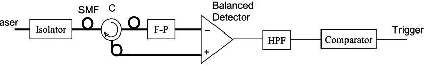
axial scan line. However, in practice, the sweep will be slightly nonlinear and direct Fourier transform of the signal sampled in equal time will result in worse resolution and SNR. Thus we chose to make a trigger generation module to generate trigger signal equally spaced in
k, as shown in Fig. 2.4. In the module, a Fabry-Perot filter (Micron Optics) is used to filter
the input laser in equally spaced k. The balanced detector is used to magnify the filtered
signal by subtracting the transmitted power from the reflected power of the Fabry-Perot filter. Finally, the electronic signal is transformed to a square wave (0 and 5 V) by the high-pass filter and the comparator. The square wave is then used as the trigger for the ADC. Note that there are different ways, including hardware based or software based methods, to solve this problem.
Isolator F-P C
SMF
+ −
HPF Comparator laser
Trigger Balanced
Detector Isolator F-P
C SMF
+ −
HPF Comparator laser
Trigger Balanced
[image:30.612.117.537.453.517.2]Detector
Figure 2.4. Schematic of trigger generation module. SMF: single-mode fiber; C: circulator; F-P: Fabry-Perot filter; HPF: high-pass filter.
The important characteristics of the swept-source based OCT system are summarized as follows: laser power = 2.5mW, center wavelength = 1300nm, bandwidth = 70nm, axial
resolution = 9.3μm, A-scan rate = 250Hz, theoretical SNR = 125dB.
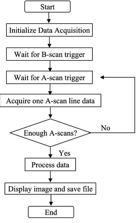
Start
Initialize Data Acquisition
Acquire one A-scan line data
Enough A-scans? No
Yes Process data
Display image and save file
End
Wait for B-scan trigger
Wait for A-scan trigger Start
Initialize Data Acquisition
Acquire one A-scan line data
Enough A-scans? No
Yes Process data
Display image and save file
End
Wait for B-scan trigger
[image:31.612.209.442.162.540.2]Wait for A-scan trigger
Figure 2.5. Flow chart of LabView program for the PARS-OCT probe imaging.
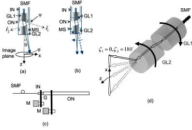
Paired-Angle-Rotation Scanning (PARS) Forward-Imaging Probe
lenses are commonly used for endoscopic imaging probes [20, 21]. Compared with other probe design, the advantages of the PARS-OCT probe are (1) large ratio of the forward-scan arc length to the probe diameter, thus allowing a large forward-scan range for a small probe; (2) large effective emission-collection numerical aperture, thus allowing high resolution for a small probe. As an example according to theoretical calculation, a well-designed probe
based on a pair of GRIN lenses with 112μm diameter with a maximum deflection angle of
20o can have an initial beam width that is 34% of the probe diameter.
(c) (d) (b) (a) ON IN G M SMF M GL2 θ ϕ GL1 GL2 SMF IN ON MS GL1 GL2 SMF IN ON MS GL1 SMF z x Image plane 2 ˆ
r rˆ1
x z o 180 , 0 2
1= ζ =
ζ ψ (c) (d) (b) (a) ON IN G M SMF M GL2 θ ϕ GL1 GL2 SMF IN ON MS GL1 GL2 SMF IN ON MS GL1 SMF z x Image plane 2 ˆ
r rˆ1
x z o 180 , 0 2
1= ζ =
[image:32.612.115.512.248.516.2]ζ ψ
Figure 2.6. Schematic of the PARS-OCT probe. (a) When there is an angle between the two angled surfaces of the GRIN lenses, the exit laser beam is tilted; (b) When the two angled surfaces of the GRIN lenses are parallel, the exit laser beam is undeviated; (c) Actuation system and the PARS-OCT setup; (d) profile of PARS-OCT B-scan mode. SMF: single-mode fiber; GL1, GL2: GRIN lenses 1 and 2; IN: inner needle; ON: outer needle; MS: metal sleeve; M, motor; G: gear.
at an angle ψ, and thus the beam is deflected. The deflected beam then enters the second GRIN lens through an identically angle-cut face of the GRIN lens, which further bends the beam. Finally, the beam exits the second GRIN lens and focuses at a point ahead of the probe. The exact position and the size of the focal point are determined by the pitches of the two GRIN lenses. For convenience, we shall define the orientations of the two GRIN lenses by angles ζ1 and ζ2, which are defined as the angles between the projections of
vectors rˆ1 and rˆ2, respectively, in the image plane and the x-axis (see Fig. 2.6(a)). We shall
also define the direction of the output light beam by its polar angle θ that it makes with the
z-axis and its azimuthal angle ϕ; an angle of θ = 0 implies that the exit beam propagates along the z-axis.
As shown in Fig. 2.6(a), when there is an angle between the two angled faces of the GRIN
lenses, the exit beam is tilted. For the special case of ζ1 = 0o and ζ2 = 180o, the exit beam
will have the largest deviation with θ = θmax and ϕ = 0. When the two GRIN lenses are
rotated simultaneously at the same speed and in opposite direction away from the starting
position of ζ1 = 0o and ζ2 = 180o, the exit beam will scan a fan sweep pattern, as shown in
Fig. 2.6(d), which can be used to acquire B-scan OCT images. Another special case is
when ζ1 = ζ2 = 90o, i.e., the two angled face of the GRIN lenses are parallel as shown in
Fig. 2.6(b), the exit beam will be undeviated. The two GRIN lenses are attached to separate concentric needles, and the rotation of the two needles are actuated by two motors and gears located far from the probe tip, as shown in Fig. 2.6(c).
The relation among θ, ζ1, and ζ2 cannot be simply expressed analytically. MATLAB
200 μm
200 μm
200 μm
Figure 2.7. Calculated B-scan mode profile as projected in the focal plane of the exit beam.
To get a simplified expression of θ, we assume that the beam is collimated by the first
GRIN lens, and then focused by the second GRIN lens. After the first GRIN lens, the angle
between the collimated beam and the axis is (α−ψ), where α sin 1( sinψ)
n
−
= . The ABCD
matrix of the GRIN lens can be written as [22], if we disregard the angled surface,
⎥ ⎥ ⎥ ⎥ ⎦ ⎤ ⎢ ⎢ ⎢ ⎢ ⎣ ⎡
− sin( ) cos( )
) sin( ) cos( 2 1 2 0 0 1 A Z n n A Z n A N A Z A N n A Z ,
where N0 and A are the on-axis refractive index and the index gradient constant of the
GRIN lens, respectively, Z is the length of the GRIN lens, and n1 and n2 are the refractive
indexes of the medium before and after the GRIN lens, respectively. In paraxial region, the ray direction (θin, θout) and height (hin, hout) before and after the GRIN lens, as indicated in
Fig. 2.8, can be calculated by the ABCD matrix as follows:
⎥ ⎦ ⎤ ⎢ ⎣ ⎡ ⎥ ⎥ ⎥ ⎥ ⎦ ⎤ ⎢ ⎢ ⎢ ⎢ ⎣ ⎡ − = ⎥ ⎦ ⎤ ⎢ ⎣ ⎡ in in out out h A Z n n A Z n A N A Z A N n A Z h θ θ ) cos( ) sin( ) sin( ) cos( 2 1 2 0 0 1
θinhin houtθout
GRIN lens
θinhin houtθout
GRIN lens
Figure 2.8. Paraxial ray tracing of GRIN lens.
To consider the effect of the angled surface, we first calculate the angle between the beam and the axis after the refraction on the angled surface of the second GRIN lens, θ1, and then
use it as the equivalent incident beam angle for unpolished surface. Assuming paraxial beam propagation, an analytical expression can be derived as
1 0
0 sin( ) tan(ψ)(α ψ) cos( ) θ
θ =−N A Z A ⋅d − +N Z A ⋅ , (2.13)
where
2 0 2
1 2
0 0 2
2 0
1 )( )sin cos( ) ( )
1 1 ( 2 sin
) 1 1 (
N N
N N
ψ α ξ ξ ψ ψ α ψ
θ = − + − − − + − . (2.14)
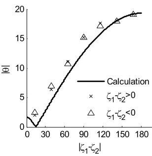
The detail calculation of θ1 is shown in appendix of this chapter. Figure 2.9 shows the
theoretically calculated and experimentally measured exit beam polar angle |θ| versus the
difference between the orientation angles of the two GRIN lenses |ζ1-ζ2|. We can see that
0 30 60 90 120 150 180 0
5 10 15 20
|ζ1-ζ2| |θ
|
Calculation
ζ1-ζ2>0
ζ1-ζ2<0
Figure 2.9. Calculated and measured exit beam polar angle, |θ|, versus the difference
between the orientation angles of the two GRIN lenses, |ζ1-ζ2|.
(a) (b)
[image:36.612.239.393.88.246.2](a) (b)
Figure 2.10. Scanning modes of the needle probe. (a) Spiral scanning, when both needles rotate at slightly different speeds and in the same direction; (b) starburst scanning, when both needles rotate at slightly different speeds but in the opposite direction.
direction with a slightly different speed (in this case, θ changes quickly while ϕ changes slowly), we can get a starburst scan pattern, as shown in Fig. 2.10(b).
0 100 200 300
0.0 0.2 0.4 0.6 0.8 1.0
Normal
ize
d o
utp
ut
po
we
r
angle difference (degrees)
0 100 200 300
0.0 0.2 0.4 0.6 0.8 1.0
Normal
ize
d o
utp
ut
po
we
r
angle difference (degrees)
Figure 2.11. The variation of the output power as the orientation of the needles changes.
3 cm
3 cm
Figure 2.12. Actuation system and the PARS-OCT probe.
shown in Fig. 2.11. We can see from the data that the maximum variation is about 3 dB. This will introduce some SNR difference for different scan lines, but the variation is still acceptable for imaging.
In our prototype PARS-OCT probe, a pair of GRIN lenses (diameter = 1 mm, SLW-1.0
from NSG America) were polished to the desired length with an angle of ψ = 22o, then
attached, using common 5-minute epoxy, to an inner needle (18XTW gauge) and an outer needle (16TW gauge) that are cut from standard hypodermic tubings (Poppers & Sons). Thus the overall probe diameter is 1.65mm. A single-mode fiber (SMF) was then angled cleaved (~8o) and attached to the back face of the GRIN lens in the inner needle. The back
face of the GRIN lens is also designed to be angled (~8o). Note that the purpose to angle
cleave the fiber and to used the angled GRIN lens is to reduce back reflection from the inner reflection inside the needle, as this will contribute to the noise of the system and reduce the SNR [23]. During fabrication, we rotated the fiber and monitored the back reflection and made sure that the position of the fiber was optimal before applying epoxy. To get a satisfactory SNR, the back reflection should be less than -45dB compared with the exit laser power. For comparison, the return losses of fiber connectors are: PC > 45dB, UPC > 50dB, APC > 60dB. Thus the back reflection of the probe should be at least better than the PC connector to get a decent SNR. The exposed needle length was 1cm in the prototype and can be easily adjusted to be up to 3cm long. Figure 2.12 shows a picture of
the actuation system and the prototype probe. The largest scan half angle θmax can be
calculated from ψ to be 19o. In our design, the on-axis pitch of the first GRIN lens (0.285) is slightly larger than 1/4 so that the beam exits from the first GRIN lens was roughly collimated (note that in this case a 1/4-pitch GRIN lens will generate a collimated beam, and a 1/4 to 1/2-pitch GRIN lens will generate a converged beam) and thus insensitive to the distance between the two GRIN lenses, which makes the fabrication easier. At the same time, the slightly convergence of the beam helps to keep the beam within the probe diameter although it is deflected. The on-axis pitch of the second GRIN lens (0.076) was chosen to be shorter than 1/4 pitch so that the exit beam was focused tightly with the desired working distance. ZEMAX simulation (ZEMAX Development) shows a focal spot
comparison, the working distance of prototype probe was measured to be 1.4mm when the exit beam is undeflected, and the focal spot size of the exit beam was measured to be
10.3μm. The difference is mainly caused by errors in the length GRIN lens during
polishing and approximated simulation of the angle-polished GRIN lens by Zemax. When the exit beam is tilted at the position of ζ1 = 0o and ζ2 = 180o, the working distance will be
slightly shorter (1.27mm), and the focal spot size will be slightly larger (12.5μm).
Detector Lens
r
Razor blade
z
Detector Lens
r
Razor blade
z
Figure 2.13. Schematic of measuring the focus size of the exit beam.
The foal spot size was measured by moving a razor blade across the beam at different axial locations to measure the beam size at the locations. As shown in Fig. 2.13, at one location
z, the power P(r) was measured versus the displacement r of the razor blade, and then the
curve P(r) was fit to an error function to get the beam size R(z). Finally the beam size data
at different locations R(z) were fit to a Gaussian beam intensity profile and to get the size of
the beam waist.
Because of the loss and internal reflections within prototype probe, the measured SNR of OCT signal (93dB) is smaller than the theoretical value (125dB). The illumination power
500
μ
m
(a)
(b)
5 mm
p
v
a
500
μ
m
(a)
(b)
5 mm
p
v
a
Figure 2.14. OCT image of the heart of a stage 54 Xenopus laevis. (a) Photograph of the
needle probe and the tadpole in experiment. (b) OCT images acquired by the PARS-OCT probe. The pixel number is 320 (transverse) × 250 (axial). p: pericardium, v: ventricle, a: atrium.
To demonstrate the capability of the prototype probe, it was used to acquire images of the
Xenopus laevis tadpole. In the experiment, we rotated the two needles with equal and
opposite angular speeds (~21rpm). Fig. 2.14(a) shows the photograph of the needle and the tadpole when acquiring the image. Figure 2.14(b) shows the OCT image of the heart of a tadpole. We can clearly discern the pericardium, ventricle and atrium in the image. Note that the image is transformed to a fan image because of the scanning profile of the probe.
(a) (c) (d)
(e) (f)
5 mm
2.5 mm
(b) c
d e f
500μm g
(a) (c) (d)
(e) (f)
5 mm
2.5 mm
(b) c
d e f
500μm
(a) (c) (d)
(e) (f)
5 mm
2.5 mm
(b) c
d e f c
d e f
500μm 500μm
[image:41.612.128.499.95.372.2]g
Figure 2.15. OCT images of the gill pockets of a stage 54 Xenopus laevis tadpole. (a)
Photograph of the probe and the tadpole when acquiring the images. (b) Indication of the scan location (c)-(f) in the tadpole. (c)-(f) OCT images acquired by the PARS-OCT probe. g: gill pockets.
To characterize a forward-scanning probe, we shall define two important parameters, RDR (scan range to probe diameter ratio) and BDR (beam diameter on the exit face to probe diameter ratio):
, diameter
Probe
face exit on the diameter Beam
BDR , diameter Probe
range Scan
RDR= = (2.15)
Figure 2.16. Definition of some parameters of the forward-scanning probe.
In summary, we have designed and implemented the paired-angle-rotation scanning (PARS) OCT probe and demonstrated its capability by acquiring OCT images of the
Xenopus laevis tadpole. Compared with other OCT endoscopic probes, the PARS-OCT
probe has numerous advantages and can be easily miniaturized. The probe can be potentially used in needle surgical procedures to provide high-resolution 3D tomographic images of the targets forward of the probe.
References
1. D. Huang, E. A. Swanson, C. P. Lin, J. S. Schuman, W. G. Stinson, W. Chang, M. R.
Hee, T. Flotte, K. Gregory, C. A. Puliafito, and J. G. Fujimoto, “Optical coherence
tomography,” Science 254, 1178-1181 (1991).
2. Z. Yaqoob, J. Wu, E. J. McDowell, X. Heng, and C. Yang, “Methods and application
areas of endoscopic optical coherence tomography,” Journal of Biomedical Optics 11,
063001 (2006).
3. G. J. Tearney, S. A. Boppart, B. E. Bouma, M. E. Brezinski, N. J. Weissman, J. F.
Southern, and J. G. Fujimoto, “Scanning single-mode fiber optic catheter-endoscope for optical coherence tomography,” Optics Letters 21, 543-545 (1996).
4. X. D. Li, C. Chudoba, T. Ko, C. Pitris, and J. G. Fujimoto, “Imaging needle for optical
coherence tomography,” Optics Letters 25, 1520-1522 (2000).
5. P. R. Herz, Y. Chen, A. D. Aguirre, K. Schneider, P. Hsiung, J. G. Fujimoto, K.
Madden, J. Schmitt, J. Goodnow, and C. Petersen, “Micromoter endoscope catheter for in vivo, ultrahigh-resolution optical coherence tomography,” Optics Letters 29,
2261-2263 (2004).
6. X. M. Liu, M. J. Cobb, Y. C. Chen, M. B. Kimmey, and X. D. Li, “Rapid-scanning
forward-imaging miniature endoscope for real-time optical coherence tomography,” Optics Letters 29, 1763-1765 (2004).
7. T. Q. Xie, H. K. Xie, G. K. Fedder, and Y. T. Pan, “Endoscopic optical coherence
tomography with a modified microelectromechanical systems mirror for detection of bladder cancers,” Applied Optics 42, 6422-6426 (2003).
Scan range Beam diameter on the exit face
8. T. A. King, and G. M. Fuhrman, “Image-guided breast biopsy,” Seminars in Surgical Oncology 20, 197-205 (2001).
9. C. P. C. Chen, S. F. T. Tang, T. C. Hsu, W. C. Tsai, H. P. Liu, M. J. L. Chen, E. Date,
and H. L. Lew, “Ultrasound guidance in caudal epidural needle placement,” Anesthesiology 101, 181-184 (2004).
10. J. Wu, M. Conry, C. Gu, F. Wang, Z. Yaqoob, and C. Yang, “Paired-angle-rotation
scanning optical coherence tomography forward-imaging probe,” Optics Letters 31,
1265-1267 (2006).
11. S. Han, M. V. Sarunic, J. Wu, M. Humayun, and C. Yang, “Handheld
forward-imaging needle endoscope for ophthalmic optical coherence tomography inspection,” Journal of Biomedical Optics 13, 020505 (2008).
12. B. E. Bouma, and G. J. Tearney, Handbook of optical coherence tomography
(Informa healthcare, 2001).
13. M. V. Sarunic, M. A. Choma, C. Yang, and J. A. Izatt, “Instantaneous complex
conjugate resolved spectral domain and swept-source OCT using 3x3 fiber couplers,” Optics Express 13, 957-967 (2005).
14. M. Wojtkowski, A. Kowalczyk, R. Leitgeb, and A. F. Fercher, “Full range complex
spectral optical coherence tomography technique in eye imaging,” Optics Letters 27,
1415-1417 (2002).
15. M. A. Choma, M. V. Sarunic, C. Yang, and J. A. Izatt, “Sensitivity advantage of
swept source and Fourier domain optical coherence tomography,” Optics Express 11,
2183-2189 (2003).
16. M. Wojtkowski, R. Leitgeb, A. Kowalczyk, T. Bajraszewski, and A. F. Fercher, “In
vivo human retinal imaging by Fourier domain optical coherence tomography,”
Journal of Biomedical Optics 7, 457-463 (2002).
17. I. Hartl, X. D. Li, C. Chudoba, R. K. Ghanta, T. H. Ko, J. G. Fujimoto, J. K. Ranka,
and R. S. Windeler, “Ultrahigh-resolution optical coherence tomography using continuum generation in an air-silica microstructure optical fiber,” Optics Letters 26,
608-610 (2001).
18. M. Wojtkowski, V. J. Srinivasan, T. H. Ko, J. G. Fujimoto, A. Kowalczyk, and J. S.
Duker, “Ultrahigh-resolution, high-speed, Fourier domain optical coherence
tomography and methods for dispersion compensation,” Optics Express 12,
2404-2422 (2004).
19. A. M. Rollins, and J. A. Izatt, “Optimal interferometer designs for optical coherence
tomography,” Optics Letters 24, 1484-1486 (1999).
20. W. A. Reed, M. F. Yan, and M. J. Schnitzer, “Gradient-index fiber-optic microprobes
for minimally invasive in vivo low-coherence interferometry,” Optics Letters 27,
1794-1796 (2002).
21. J. C. Jung, and M. J. Schnitzer, “Multiphoton endoscopy,” Optics Letters 28, 902-904
(2003).
22. W. L. Emkey and C. A. Jack, “Analysis and Evaluation of graded-index fiber-lenses,”
Journal of Lightwave Technology 5, 1156-1164 (1987).
23. K. Takada, “Noise in optical low-coherence reflectometry,” IEEE Journal of Quantum
Appendix A: Derivation of Equation (2.14)
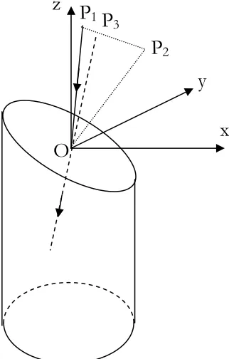
Figure 2A.1.Refraction at the angled face of the second GRIN lens. P1O is the incident ray,
P3O is the refracted ray, and P2O is the surface normal.
The refraction happened at the angled face of the second GRIN lens can be illustrated in Fig. 2A.1. Suppose the z-axis is along the axis of the GRIN lens, and the incident ray is at
the xz-plane. The incident ray is P1O, the refractive ray is P3O, and the surface normal is
OP2. We choose P1 and P2 such that OP1 = OP2 = 1, and P3 is at the line of P1P2. At small
angle approximation, |OP3| ≈ 1. We already know that the angle between incident ray P1O
and the z-axis is α-ψ, so the coordinates of P1 can be written as
)) cos(
, 0 ),
(sin(α −ψ α −ψ . Assuming the angle between the projection of OP2 in the xy
-plane and the x-axis is φ, then the coordinates of P2 are (sinψ cosφ,sinψ sinφ,cosψ). Our
goal is to calculate the coordinates of P1, (x, y, z), such that the angle θ1 and the orientation
of the refractive ray can be calculated. Let γ be the angle between P1O and OP2, i.e., the
incident angle for refraction, and β be the angle between P3O and OP2, i.e., the refractive
angle. In small angle approximation, we have
x
z
y
O
P
1P
20 2 1 3 2 1 N P P P P ≈ ≈ γ β
. (2A.1)
Here we use the Snell’s law, and N0 is the center refractive index of the GRIN lens.
Obviously, the coordinates P1, P2, and P3 satisfy
. 1 ) cos( cos cos sin sin sin sin ) sin( cos sin cos sin 0 2 1 3 2 N P P P P z y x ≈ = − − − = − = − − − ψ α ψ ψ φ ψ φ ψ ψ α φ ψ φ ψ (2A.2)
Here we use Eq. (2A.1). Thus
). cos( 1 cos ) 1 1 ( , sin sin ) 1 1 ( , ) sin( cos sin ) 1 1 ( 0 0 0 0 0 ψ α ψ φ ψ ψ α φ ψ − + − = − = − + − = N N z N y N N x (2A.3)
So the angle θ1 satisfies
. ) ( ) ( cos sin ) 1 1 ( 2 sin ) 1 1 ( ) ( sin ) sin( cos sin ) 1 1 ( 2 sin ) 1 1 ( sin 2 0 0 0 2 2 0 2 0 2 0 0 2 2 0 2 2 3 2 2 1 1 N N N N N N N N y x OP y x ψ α ψ α φ ψ ψ ψ α ψ α φ ψ ψ θ θ − + − − + − ≈ − + − − + − = + ≈ + = ≈ (2A.4)
Now using the relation φ =ξ1−ξ2, we get the Eq. (2.14). Note that by knowing (x, y, z),
we can also calculate the azimuthal angle ϕ of the exit beam by
2 2 1 cos y x x + = −
In the above calculation, we can also remove the approximations and calculated the θ1
C h a p t e r I I I
FULL-FIELD PHASE IMAGING PRINCIPLE WITH HARMONICALLY MATCHED DIFFRACTION GRATING (G1G2 GRATING)
Compared with intensity imaging, quantitative phase imaging has the advantages of high sensitivity and high resolution. Because phase techniques are sensitive to the optical path length instead of the intensity change, they are widely used to study transparent samples, such as living cells. Phase techniques can also be used in metrology as they can provide higher resolution than intensity based techniques in many situations. The success of phase contrast microscopy and differential interference contrast microscopy has proved the efficacy of phase techniques in studying biological samples. The development of various quantitative phase methods further shows the potential capacity of phase techniques in many applications. In this chapter, I will focus on the full-field quantitative phase imaging techniques that are developed in our lab using a harmonically matched diffraction grating (G1G2 grating) [1-3]. Compared with other phase imaging methods, our technique has many advantages: (1) Imaging speed is limited only by the camera’s speed, as phase image are reconstructed from two camera images acquired simultaneously. In comparison, the speed of phase shifting interferometry method is additionally limited by the phase stepping process [4]. (2) Allowing full field-of-view phase imaging, unlike some other techniques such as digital holography, where the tilt of reference beam can limit the field-of-view [5]. (3) The G1G2 grating is a planar device and can be easily designed and fabricated.
Overview of Related Phase-Imaging Techniques
Holography was invented by Gabor [6] about half a century ago and has been widely used especially after the invention of laser. Conventional holography uses holographic materials for recording the holograms. Recent years researchers began using digital recording devices such as CCD cameras to record the holograms and can thus obtain quantitative phase and intensity information of the sample. The technique is called digital holography and its schematic is shown in Fig. 3.1.
Sample
CCD
Sample beam
Reference beam
Sample
CCD
Sample beam
Reference beam
Figure 3.1. Schematic of digital holography.
The interferogram on the CCD camera can be written as
* *
2 2
RS S R S R
I ∝ + + + , (3.1)
where R and S are the complex amplitudes of the electric field of the reference beam and the sample beam, respectively. The first two terms in Eq. (3.1) are DC terms, and the last two terms are interference terms. After recording of the interferogram, the sample beam can then be reconstructed by multiplying the reference field to the interferogram:
* 2 2 2
2
S R S R R S R R
IR∝ + + + . (3.2)
reference beam and the sample beam. The angle will have to be large enough such that the different components can be separated spatially and be small enough such that the high-frequency fringes can be discerned by the CCD camera. The last two terms can then be digitally propagated by the Fresnel integral to obtain the phase and intensity information of the sample.
From the above description we can see that the off-axis scheme is critical for digital holography. However, the high-frequency fringes on the CCD camera effectively result in inefficient use of the pixels since several pixels have to be used to record one fringe that contains both the phase and intensity information. The off-axis scheme also limits the spatial resolution of the image because high resolution image corresponds to high spatial frequency of the fringes, and the achievable frequency of the fringes is limited by the pixel size of the CCD camera.
To overcome the abovementioned disadvantages of the off-axis holography, in-line holography is also developed. In this case, a phase shifting is often used to extract the phase information [7]. However, the phase-shifting process will need additional time and might introduce additional noise.
To obtain the phase information without the phase-shifting process, 3 × 3 fiber coupler-based technique has been developed [8, 9]. The schematic of the interferometer is shown in Fig. 3.2.
Figure 3.2. Interferometer based on 3 × 3 fiber coupler
Sample beam Reference beam
Port 1
Port 2
Assuming the 3 × 3 fiber coupler is ideal and the split ratio is the same for the output ports, the interference signals at the output ports can be written as
Port 1: )
3 2 cos(
3 2 3 3 1
π ψ ψ − − +
+
= r s s r
s r
P P P
P
P , (3.3)
Port 2: cos( )
3 2 3 3
2 r s s r
s r
P P P
P
P = + + ψ −ψ , (3.4)
Port 3: )
3 2 cos(
3 2 3 3 1
π ψ ψ − + +
+
= r s s r
s r
P P P
P
P , (3.5)
where Pr and Ps are the input powers of reference and sample beam, respectively; ψr and ψs are the phases of the reference beam and sample beam before the fiber coupler. We can see that the interference signals at the three output ports have a phase shift of 120o among one another. This is effectively equivalent to a phase shifting interferometer and the phase and intensity information can be easily calculated directly from the detected interference signals.
We note that the 3 × 3 fiber coupler-based interferometer has to be combined with scanning mechanism to acquire 2D images. This motivates us to look for its full-field equivalent such that a 2D image can be obtained without scanning.
Harmonically Matched Diffraction Grating
Consider a simple interferometer as shown in Fig. 3.3(a), where a common beamsplitter is used to split and combine the reference beam and the sample beam, the interference signals at the output ports can be expressed as:
Port1: P1 =Pr /2+Ps /2+ PrPs cos(ψs −ψr), Port2: P2 =Pr /2+Ps/2− PrPs cos(ψs −ψr),
(3.6) (3.7)
the two interference terms are trivially related, it is generally impossible to extract phase information from this simple interferometer without resorting to some form of phase encoding.
Sample beam
Reference beam Port 1
Port 2
diffraction grating
Sample beam
x
z y
Reference beam
Port 1
Port 2
(a) (b)
Sample beam
Reference beam Port 1
Port 2 Sample beam
Reference beam Port 1
Port 2
diffraction grating
Sample beam
x
z y
Reference beam
Port 1
Port 2 diffraction grating
Sample beam
x
z y
x
z y
Reference beam
Port 1
Port 2
(a) (b)
Figure 3.3. (a) Simple interferometer based on common beamsplitter; (b) interferometer based on single shallow grating.
The trivial phase shift of the two output ports can also be understood by noticing the conservation of energy of the input and output power. Thus, in principle, the output of two ports systems would be trivially rela