Learning for Frequency Domain Optical Coherence
Tomography
Thesis by
Sinan Zhao
In Partial Fulfillment of the Requirements
for the Degree of
Doctor of Philosophy
California Institute of Technology
Pasadena, California
2016
©2016 Sinan Zhao
My time at Caltech has been a transforming experience, at all levels. I’m blessed
with the fortune to meet and interact with a number of great people, who I would
like to take the opportunity to acknowledge here. Caltech is such a wonderful and
resourceful place that, even if you only have a vague idea about what you want to
achieve, it is able to help you crystallize your thoughts and materialize your dreams.
First and foremost, my sincere thanks are due to my advisor Prof. Amnon Yariv,
who admitted me to Caltech, introduced me to the field of optoelectronics, and
al-lowed me to pursue freely my interests in the field of machine learning, applied
math-ematics, and computer science. Without his support and encouragement, this thesis
would not have been possible. His guidance, challenging questions, and suggestions
has greatly accelerated my development as a researcher and allowed me to flourish
both professionally and intellectually.
Not only is Prof. Yariv a gifted scientist, he is also a such versatile man that all of
us wish to emulate: he is capable of speaking seven languages and knows just about
everything of history and art (he even gave us a lecture about classical music on an
applied physics class), not to mention that he has been an expert in surfing and has
traveled all around the globe, including the Antarctic. His unique and well-rounded
experience has inspired us from the highest level and motivated us to always take a
step further.
My special thanks are due to Prof. Yaser Abu-Mostafa, who has made great
influences on me during my journey at Caltech. Meeting Yaser was an absolute
turning point of my life and career. Not only did he introduce me to the exciting field
His on-line courseLearning From Data is so intriguing that you cannot help watching it time and time again. The quality of the course is certainly way off the chart,
but at the same time it just feels great to hear that man talking. The half year
span where I could meet Yaser several times a week working on an industrial project
definitely ranks high among my best times at Caltech. Yaser is the ultimate guru
in solving real-world machine learning problems. His level of expertise and wisdom
makes working with him the most enjoyable and rewarding experience you could ever
ask for, and also his attention to technical details renders him the ideal boss. I will
never forget the time when I had an idea in the middle of the night for the project,
and discovered that Yaser was still at his office, ready for an immediate discussion
with me.
I thank Profs. Bruno Crosignani, P. P. Vaidyanathan, Willie Ng for being part of
my thesis committee, as well as Prof. Mark Simons who was part of my candidacy
committee. I enjoyed working with Prof. Bruno Crosignani on solving interesting
physics problems, along with the fun discussions regarding how to help me improve
my taste of wine. I thank Prof. Willie Ng for collaborating with us on the iPhod
project while he was at HRL Laboratories.
I would like to thank the Caltech departments and professors who employed me
as a Teaching Assistant. Without their help it won’t be possible for me to survive
these years. I’m especially grateful for Prof. Houman Owhadi, who has employed me
three times as his TA. I even gave a graduate-level lecture at Caltech on his behalf
while he was out of town, and I still remember my nervousness on that occasion. I
also thank the head TAs of ACM95/100, Gerardo Cruz and Adam Neumann, and
Maria Lopez at Computing & Mathematical Sciences, for constantly looking after me
in case I need a TAship each and every term.
My thanks are also due to the Yariv group members, both old and new -
Xi-ankai Sun, Naresh Satyan, Hsi-Chun Liu, Christos Santis, Arseny Vasilyev, Jacob
Sendowski, Mark Harfouche, Dongwan Kim, Marilena Dimotsantou, Paula Popescu,
Reg Lee, and George Rakuljic - for their help and friendship, for all of the
Zhao Liu, Dongyang Kang, Xin Ning, Zhenhua Liu, Jiang Li, Maolin Ci, Dunzhu Li,
Chenguang Ji, Kuang Shen, as well as the CaltechC 2010 members, for all the fun
we had together and the memories we shared, they are so priceless and will stick in
my mind for the years to come.
I would like to thank my parents, who have always been there for me throughout
my years abroad. I will be forever grateful for their constant love and unconditional
support.
Lastly, I would like to express my deepest thanks and gratitude to my lovely
wife, Shuang (Vivian) Wu. This thesis would not have been possible without her
encouragement, sacrifice, and love. She is such a fun character and at the same time
extremely talented. There are an endless number of things that I could learn from her,
from Japanese to classical music, from singing to playing piano, not to mention that
she also manages to beat me in heads-up poker from time to time, which is completely
unconceivable. My life would never be out of joy with her company. Meeting her in
Pasadena and living with her at Caltech has been the most wonderful thing ever
Abstract
Optical Coherence Tomography(OCT) is a popular, rapidly growing imaging
tech-nique with an increasing number of biomedical applications due to its noninvasive
nature. However, there are three major challenges in understanding and improving
an OCT system:
• Obtaining an OCT image is not easy. It either takes a real medical experiment
or requires days of computer simulation. Without much data, it is difficult to
study the physical processes underlying OCT imaging of different objects simply
because there aren’t many imaged objects.
• Interpretation of an OCT image is also hard. This challenge is more profound
than it appears. For instance, it would require a trained expert to tell from an
OCT image of human skin whether there is a lesion or not. This is expensive
in its own right, but even the expert cannot be sure about the exact size of the
lesion or the width of the various skin layers. The take-away message is that
analyzing an OCT image even from a high level would usually require a trained
expert, and pixel-level interpretation is simply unrealistic. The reason is simple:
we have OCT images but not their underlying ground-truth structure, so there
is nothing to learn from.
• The imaging depth of OCT is very limited (millimeter or sub-millimeter on
human tissues). While OCT utilizes infrared light for illumination to stay
non-invasive, the downside of this is that photons at such long wavelengths can
only penetrate a limited depth into the tissue before getting back-scattered.
re-Monte Carlo simulation platform which is 10,000 times faster than the
state-of-the-art simulator in the literature, bringing down the simulation time from 360 hours to a
single minute. This powerful simulation tool not only enables us to efficiently generate
as many OCT images of objects with arbitrary structure and shape as we want on
a common desktop computer, but it also provides us the underlying ground-truth of
the simulated images at the same time because we dictate them at the beginning of
the simulation. This is one of the key contributions of this thesis. What allows us
to build such a powerful simulation tool includes a thorough understanding of the
signal formation process, clever implementation of the importance sampling/photon
splitting procedure, efficient use of a voxel-based mesh system in determining
photon-mesh interception, and a parallel computation of different A-scans that consist a
full OCT image, among other programing and mathematical tricks, which will be
explained in detail later in the thesis.
Next we aim at the inverse problem: given an OCT image, predict/reconstruct
its ground-truth structure on a pixel level. By solving this problem we would be able
to interpret an OCT image completely and precisely without the help from a trained
expert. It turns out that we can do much better. For simple structures we are able
to reconstruct the ground-truth of an OCT image more than 98% correctly, and for
more complicated structures (e.g., a multi-layered brain structure) we are looking at
93%. We achieved this through extensive uses of Machine Learning. The success of
the Monte Carlo simulation already puts us in a great position by providing us with a
great deal of data (effectively unlimited), in the form of (image, truth) pairs. Through
a transformation of the high-dimensional response variable, we convert the learning
task into a multi-output multi-class classification problem and a multi-output
(committee of experts) and train different parts of the architecture with specifically
designed data sets. In prediction, an unseen OCT image first goes through a
clas-sification model to determine its structure (e.g., the number and the types of layers
present in the image); then the image is handed to a regression model that is trained
specifically for that particular structure to predict the length of the different layers
and by doing so reconstruct the ground-truth of the image. We also demonstrate that
ideas fromDeep Learning can be useful to further improve the performance.
It is worth pointing out that solving the inverse problem automatically improves
the imaging depth, since previously the lower half of an OCT image (i.e., greater
depth) can be hardly seen but now becomes fully resolved. Interestingly, although
OCT signals consisting the lower half of the image are weak, messy, and
uninter-pretable to human eyes, they still carry enough information which when fed into a
well-trained machine learning model spits out precisely the true structure of the object
being imaged. This is just another case where Artificial Intelligence (AI) outperforms
human. To the best knowledge of the author, this thesis is not only a success but
also the first attempt to reconstruct an OCT image at a pixel level. To even give a
try on this kind of task, it would require fully annotated OCT images and a lot of
them (hundreds or even thousands). This is clearly impossible without a powerful
Acknowledgements iv
Abstract vii
Glossary of Acronyms xxv
1 Overview 1
1.1 Introduction . . . 1
1.2 Basic OCT Principle . . . 1
1.3 Present Challenges in OCT . . . 3
1.4 Summary of Our Contributions . . . 6
1.5 Organization of the Thesis . . . 9
2 Understanding the OCT Signal 12 2.1 Chapter Overview . . . 12
2.2 Signal Formation in FD-OCT Systems . . . 12
2.2.1 A Toy Example . . . 14
2.2.2 Another Toy Example with Two Targets . . . 16
2.3 From Mirrors to Biological Tissues . . . 18
2.3.1 Photon Path Length Becomes A Distribution . . . 20
2.3.2 A-scans Are No Longer Identical . . . 21
2.4 Reasons for the Need of Simulation . . . 23
3.2 Introduction . . . 24
3.3 Basic Principles and the Monte Carlo Engine . . . 26
3.3.1 Overview of the Simulation Steps . . . 26
3.3.2 Mathematical Details of Implementation . . . 27
3.3.3 More Complex Geometry . . . 29
3.3.4 OCT Transverse and Axial Signal Localization . . . 30
3.3.5 OCT Angiography and Blood Flow Simulation . . . 32
3.3.6 Putting It Together . . . 33
3.4 Class I and Class II Photons . . . 34
3.5 Why the Simulation is Slow . . . 36
3.5.1 FD-OCT vs TD-OCT . . . 36
3.5.2 Calculation of the Reflectance in TD-OCT . . . 37
3.5.3 Discussion . . . 38
4 Speeding up the Monte Carlo 40 4.1 Chapter Overview . . . 40
4.2 Three Challenges . . . 40
4.3 Importance Sampling and Photon Splitting . . . 41
4.3.1 Introduction . . . 42
4.3.2 Mathematical Details . . . 42
4.3.3 Additional biased scatterings . . . 45
4.3.4 Photon Splitting . . . 45
4.3.5 Calculation of the reflectance . . . 47
4.3.6 Generation of random biased angles . . . 48
4.4 Identifying Photon-Mesh Intersection . . . 48
4.5 Parallelization of A-Scans . . . 50
4.6 Simulation Results . . . 51
5 The Learning Problem 56 5.1 Chapter Overview . . . 56
5.4 Discussion . . . 69
6 Solving the Learning Problem 71 6.1 Chapter Overview . . . 71
6.2 First Impression and Initial Thoughts . . . 72
6.3 Transformation of the Output . . . 73
6.4 Three Data Sets . . . 75
6.5 Decision Trees, Random Forest, Extra Trees . . . 77
6.5.1 Introduction to Decision Trees . . . 77
6.5.2 Mathematical Formulation of Decision Trees . . . 78
6.5.3 Ensemble methods . . . 80
6.6 Exploring and Shuffling the Data . . . 82
6.6.1 Initial Exploration . . . 82
6.6.2 Shuffling the Data . . . 83
6.6.3 Transfer Learning . . . 84
6.7 Restricted Boltzmann Machines . . . 85
6.8 Hierarchical Architecture . . . 86
6.8.1 Predicting the Length of the Segments . . . 87
6.8.2 Interpreting the RMSE . . . 88
6.8.3 From Good to Bad . . . 88
6.8.4 Committee of Experts . . . 89
6.9 Prediction Results . . . 90
7 Conclusion and Outlooks 95 7.1 Chapter Overview . . . 95
7.2.1 Simulating the Brain Structure . . . 95
7.2.2 Predicting the Brain Structure . . . 96
7.2.3 The Curved Brain Structure . . . 98
7.3 Conclusion of the Thesis . . . 98
7.4 Outlook . . . 106
A Implementation Details of the Monte Carlo Engine 108 A.1 Overview . . . 108
A.2 Coding in MATLAB . . . 108
A.3 Coding in Standard C . . . 110
B Source Code in Standard C 119 B.1 Declaration of Functions . . . 119
B.2 Major Cycle of the Monte Carlo Engine . . . 119
1.1 (A) A Michelson interferometer. (B) A Michelson interferometer with
the fixed mirror replaced by a sample. An OCT image (B-scan) of the
sample is shown below the detector. . . 2
1.2 An example of a nodular BCC lesion that was easily delineated laterally
with OCT is shown. The black arrow points at the lesion in the clinical
photo and at the same lesion in the OCT image. In between, the image
from the OCT probe is seen with a green line indicating where the OCT
scan was performed. White arrows indicate the adjacent normal skin in
the OCT image. . . 4
2.1 A FD-OCT system. The output light field is split by a diffraction
grat-ing, and component frequencies are detected by a linear detector array. 13
2.2 Time evolution of the optical frequencies of the launched and reflected
waves in a single-scatterer OCT experiment [12]. . . 14
2.3 A toy example illustrating the FD-OCT Principle. In this simple setup,
photons are emitted from different lateral positions of the source and
then collected by an array of detectors, representing different A-scans.
The sample only consists one mirror like, specular reflective target,
lo-cated at depth z0. . . 15
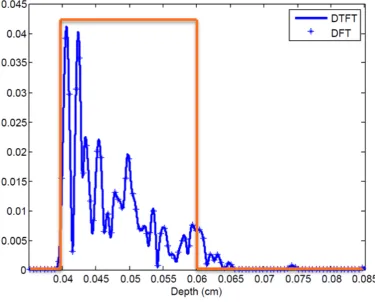
2.4 Image formation process for the toy example with a single target. (a)
histogram of the photon pathlength; (b) OCT signal at the detector; (c)
DTFT of the OCT signal, zoomed in to show the presence of the target;
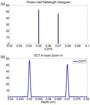
2.5 Image formation process for the toy example with two targets. (a)
his-togram of the photon half pathlength; (b) DTFT of the OCT signal at
the detector, which gives us A-scan, displaying the two distinct targets; 17
2.6 OCT Image formed by the toy example with two mirror like targets,
consisted of 256 A-scans, where each A-scan has 100 contributing photons. 18
2.7 OCT Image formed by the toy example with two mirror like targets,
consisted of 256 A-scans, where each A-scan has 1000 contributing photons. 19
2.8 OCT imaging in a more realistic setting. The previous two mirror-like
targets are replaced with a layers of biological tissue, located from depth
z0 to z1. . . 19
2.9 Image formation process for the example with one layer of biological tissue as the target. (a) histogram of the photon half pathlength; (b) OCT signal at the detector; (c) DTFT of the OCT signal, zoomed in to show the presence of the target; (d) DTFT of the OCT signal, zoomed out to show the entire A-scan. . . 20
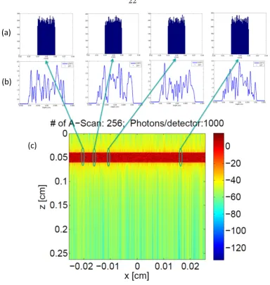
2.10 OCT Image formed by stitching 512 A-scans from the example with one layer of biological tissue as the target. (a) Top row: histograms of the photon half pathlength; (b) middle row: A-scans at different positions; (c) bottom row: the full OCT image formed by 512 A-scans. . . 22
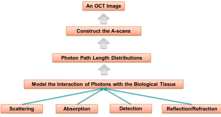
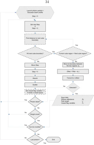
2.11 Flow chart of the modeling process. . . 23
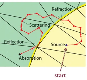
3.1 Illustration of the series of events that a photon experiences once it enters a biological tissue. . . 25
3.2 The optical properties of tissues. . . 25
3.3 Flow chart of the MC algorithm. . . 34
3.4 Class I and Class II photons. . . 35
4.1 Schematic representation of the vectors and the angles used in the bias procedure. . . 44
Class I and (b) Class II reflectance-based B-scan OCT image of the
non-layered object; (c) Spatial structure of the object; (d) Optical parameters
of the non-layered object used in the tetrahedron-based OCT simulator;
(e) A depiction of the tetrahedrons representing the non-layered object. 52
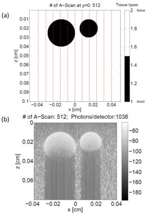
4.4 Simulated blood vessels. (a) Two blood vessels modeled at a depth of
250µm and 200µm. (b) Structural OCT image of two cylindrical blood
vessels (outlined in yellow) surrounded by a homogeneous sample. The
parameterµsfor blood is fixed to 650 cm−1,µa , to 5 cm−1,g, to 0.9888,
and n, to 1.37. The parameter µs for the sample is set to 10 cm−1, µa,
to 1 cm−1,g, to 0.7, and n, to 1.37. Scale bars correspond to 100 µm. . 54
4.5 Same blood vessels simulated using our advanced Monte Carlo platform,
consisting of 512 A-scans. The simulation only takes one minute. (a)
Two blood vessels modeled at a depth of 250 µm and 200 µm. The red
lines represent the range covered by the A-scans. (b) Structural OCT
image of two cylindrical blood vessels surrounded by a homogeneous
sample. The simulation parameters are the same as in [1], where µs for
blood is fixed to 650 cm−1, µa , to 5 cm−1,g, to 0.9888, and n, to 1.37.
The parameter µs for the sample is set to 10 cm−1,µa, to 1 cm−1, g, to
0.7, andn, to 1.37. Scale bars correspond to 100 µm. . . 55
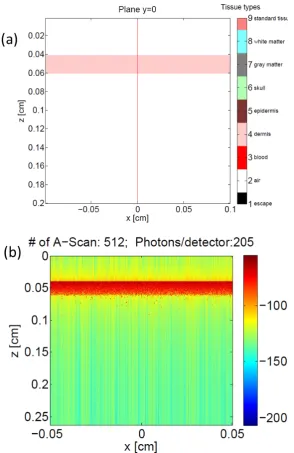
5.1 Monte Carlo simulation of a single layer biological tissue (dermis). The
OCT image consists 512 A-scans and the simulation time is one minute.
(a) Schematic drawing of the anatomical, ground-truth structure. (b)
5.2 An example A-scan from the simulated OCT image of the one-layer
biological tissue. The line in orange shows the corresponding
ground-truth structure of this A-scan. . . 58
5.3 The weighted half path length histogram of the example A-scan from
the simulated OCT image of the one-layer biological tissue. The photon
half path lengths are weighted by the weight Wi and the likelihood ratio
Li they carry. . . 59
5.4 Schematic illustration of flood Illumination. (a) The radius of the
il-lumination source equals 0.04 cm. (b) The radius of the ilil-lumination
source equals 0.08 cm. . . 60
5.5 Example A-scans under the condition of flood illumination combined
with the idea of sliding window prediction. (a) The resulting A-scan
when the radius of the illumination source equals 0.04 cm. The orange
line depicts the corresponding ground truth and the green window with
an arrow illustrates the idea of sliding window prediction. (b) Schematic
drawing of sliding window prediction, where the tissue type is predicted
one at a time using a sliding window going from left to right. . . 62
5.6 Schematic drawing of the anatomical, ground-truth structure of a
multi-layered biological tissue (three layers of dermis), where the three dermis
layers are centered at depth z = 0.02 cm, z = 0.04 cm, and z= 0.07 cm
respectively, all with a thickness of 0.01 cm. . . 63
5.7 Monte Carlo simulation of a multi-layered biological tissue structure
(three layers of dermis). The OCT image consists 512 A-scans and the
simulation time is 32 minutes. (a)Simulated OCT image displayed in
gray scale. (b) Simulated OCT image displayed in color scale. . . 64
5.8 An example A-scan from the OCT image of the three-layered tissue
structure, plotted at the dB scale. . . 65
5.9 Weighted half path length histogram at dB scale for the three-layered
i.e., predicting the ground-truth structure from an unseen OCT image. 68
5.12 The machine learning problem at the A-scan level, where we need to
predict the ground-truth structure (green line) from the transformed
OCT signal, namely the A-scan (blue line). . . 69
6.1 Reminder of the machine learning problem at the A-scan level, where
the goal is to predict the ground-truth structure, a 1910-dimensional
vector yi(green line), from the input xi (blue line), which is also a a
1910-dimensional vector. . . 72
6.2 Transformation of the 1910-dimensional output variable y into two
20-dimensional variables ytype and ylength. ytype encodes the types of the
segments of the output y into 20 class labels, and ylength describes the
length of these segments in pixels. Here the code “2” means “air” and
the code “4” means “dermis”. There is no loss of information in this
transformation as the new, lower dimensional variables ytype and ylength
are enough to fully reconstruct the original output variable y. . . 74
6.3 Three data sets for the layered, air-dermis structure. The first data set
consists of 100 OCT images where each image is composed of 512
A-scans. The images may consist 1 to 5 layers of dermis, where the dermis
layer will have a random position and a random thickness. Data set
No.2 is the same as data set No.1 except for this time there are 1000
images and each image is composed of 64 A-scans. Data set No.3 is
the same as data set No.2 except that they all have a fixed, 3 layers of
6.4 Decision Trees on IRIS data set [2], which consists of 150 samples and
3 class labels. Each sample has 4 features. . . 78
6.5 Zero-One Error for the prediction of ytype. In this case we get 4 class
labels wrong out of 20, resulting in an error probability of 0.2. . . 82
6.6 Schematic drawing of Restricted Boltzmann machines, where vi are
called visible nodes and hj hidden nodes. The weights wij connects
the two type of nodes. . . 86
6.7 Schematic drawing of the problem of predicting the length of the
seg-ments. We use the Root Mean Squared Error (RMSE) for this task. . . 87
6.8 Different test cases for theylengthprediction on Data Set No.4, where we
see some very good examples as well as very bad examples. . . 88
6.9 The hierarchical architecture in the form of a committee of experts,
where the job of the Classification Model on the top layer to dictates the
structure of the imaged object in terms of the number and type of the
segments, and assign a Regression Expert to solve the segment length
prediction problem corresponding to that particular structure. . . 89
6.10 Histogram of the RMSE on Data Set No.5, where we see that the median
RMSE is only 18.5833 compared to the average RMSE of 27.54875. This
shows that there are a few bad examples driving the RMSE up, but they
are a minority. . . 90
6.11 Histogram of the RMSE on newly generated Data Set No.5 without
those tricky cases that have layers close to the boundary. We see that
the average and median of RMSE are further reduced. However, there
are still outliers present but significantly less. . . 91
6.12 An example A-scan comparing our prediction result against the
ground-truth. This represents a typical performance of our hierarchical model. 92
6.13 An example A-scan comparing our prediction result against the
ground-truth. This represents a slightly worse-than-average performance of our
that drives the RMSE up. . . 94
7.1 Schematic drawing of the anatomical, ground-truth structure of a
multi-layered brain, which consists of an epidermis layer, a dermis layer, a skull
layer, and both white and gray matters. . . 96
7.2 Simulated OCT images corresponding to the multi-layered brain
struc-ture, which consists of an epidermis layer, a dermis layer, a skull layer,
and both white and gray matters. . . 97
7.3 An example A-scan comparing our prediction result against the
ground-truth, for the brain structure. This represents a typical performance of
our hierarchical model. . . 98
7.4 Part One of the story line. (a) An OCT image of the brain, this is what
you see. (b) The ground-truth anatomical structure of the brain, this is
what you would like to see. . . 99
7.5 Part Two of the story line. This is what you get from our machine
learning model. In our case, what you see is (almost) what you’ll get. (a)
The predicted ground-truth structure before pooling. (b)The predicted
ground-truth structure after pooling. . . 100
7.6 Schematic drawing of the anatomical, ground-truth structure of a curved
brain, which consists of an epidermis layer, a dermis layer, a skull layer,
and both white and gray matters. . . 101
7.7 Simulated OCT images corresponding to the curved brain structure,
which consists of an epidermis layer, a dermis layer, a skull layer, and
7.8 Predicted ground-truth structure (without pooling) for the curved brain
example. . . 103
6.1 Prediction Results for ytype on Data Set No.1 . . . 82
6.2 Prediction Results for ytype on Data Set No.2, which has 1000 images
and 64 A-scans per image, using Extra Trees. . . 83
6.3 Prediction Results for ytype on Data Set No.4, which has 4000 images
and 16 A-scans per image, using Extra Trees. . . 84
6.4 Prediction Results forytypeon Data Set No.4, which has 4000 images and
16 A-scans per image, using two layers of RBM with 512 components,
followed by Logistic regression. . . 86
6.5 Prediction Results for ylength on Data Set No.4, which has 4000 images
Listings
5.1 Filter the outliers among the detected photon packets with huge
like-lihood ratios. . . 60
6.1 MATLAB code for transforming the output variabley. The code
sim-ply locates the discontinuities and use the positions of them to figure
out ytype and ylength. . . 75
A.1 Create Tissue Strcture. . . 108
A.2 Computation of OCT signals and A-scans. . . 109
A.3 Initialize photon position and trajectory . . . 110
A.4 Compute the step size the photon will take to get the first voxel crossing
in one single long step. We also check whether the photon packet is
detected by the assigned detector. . . 111
A.5 Spin and Split. The Spin process is to scatter photon into new
trajec-tory defined by θ and ψ. θ is specified by cos(θ), which is determined
based on the Henyey-Greenstein scattering function, and then convert
θ and ψ into cosines ux, uy, uz. Split follows exactly the procedure
described in Section 4.3, where we apply biased backward-scatterings
and biased forward-scattering, as well as unbiased scatterings. Once
the first biased backward-scattering takes place, we split the photon
packet into two if the likelihood ratio of the biased back-scattering is
less than 1. We save the information of the continuing photon and
continue to track the current photon, by applying biased and unbiased
forward-scatterings. . . 112
Glossary of Acronyms
OCT Optical Coherence Tomography
TD-OCT Time Domain Optical Coherence Tomography
FD-OCT Frequency Domain Optical Coherence Tomography
MC Monte Carlo
ML Machine Learning
DT Decision Trees
Overview
1.1
Introduction
Optical Coherence Tomography (OCT) is rapidly becoming an important imaging
technique for numerous medical and biological applications [3, 4]. It is a sub-surface
imaging technique that uses either a low-coherence light source (time-domain
sys-tems) or a wavelength-swept laser source (frequency-domain syssys-tems). It can provide
real-time imaging and with a depth resolution of 1µm or less [5, 6], which is two
or-ders of magnitude higher resolution than ultrasound imaging. The penetration depth,
which is highly tissue-dependent, can reach up to 3 mm and is typically limited to a
few millimeters. OCT is also able to produce images inside the body when integrated
with optical fiber probes. The use of infrared and visible light is safer to most
biolog-ical samples than ionizing radiation like X-rays or gamma rays, and it also allows for
spectroscopic characterization of an object, e.g., a tumor in tissue [7]. A recent
thor-ough review of OCT technology, including frequency-domain OCT, and applications
of OCT can be found in the Handbook of Non-invasive Methods and the Skin [8].
1.2
Basic OCT Principle
OCT is an interferometric technique, relying on interference between a split and
later re-combined broadband optical field. The principle of OCT is shown in Figure
light to interfere with itself, i.e., the ability to amplify or blur itself (“constructive”
and “destructive” interference, respectively). Light is split into two paths using a
beam-splitter (half-transparent mirror). The two beams recombine at the
beam-splitter, and detected. Interference between the two reflections is possible only when
the path-lengths of the two arms are matched within the so-called coherence length
of the light source. The coherence length is determined by the spectral width of
the light—a broad optical spectrum corresponds to a short coherence length, and a
narrow optical spectrum corresponds to a long coherence length. When using a light
source with a large coherence length, interference arises for even very large differences
in path-length. When using a source with small coherence length, interference only
arises when the two path-lengths are matched within the coherence length of the
light, which may be micrometer size. It is exactly this effect that is used in OCT
for distinguishing signals from different depths of the sample. The axial resolution is
essentially the coherence length, so that a small coherence length corresponds to high
axial resolution.
Figure 1.1. (A) A Michelson interferometer. (B) A Michelson interferometer with the
fixed mirror replaced by a sample. An OCT image (B-scan) of the sample is shown
below the detector.
If one of the mirrors in the Michelson interferometer is replaced by a biological
moving the scanning mirror, the coherence gate successively selects an interference
signal from different depths. In this way, a depth scan recording can be obtained,
also referred to as an A-scan. The depth scanning range is limited by the mirror
displacement. Transverse resolution is determined by the spot size, which is given by
the focusing optics.
Two-dimensional data are obtained by moving the beam across the sample and
acquiring data (B-scan). By translating the beam in 2 directions over a surface area,
3-dimensional data can be acquired (C-scan). Acquiring 2-and 3-dimensional data
is in general possible in real-time. The interference signal is amplified, filtered to
improve the signal-to-noise ratio, and then digitized and transferred to a computer.
From the digital signal, the reflection strength is extracted and mapped, using either
a gray scale or color palette, thereby generating an OCT image [9].
1.3
Present Challenges in OCT
In Figure 1.2 we illustrate a typical clinical trial of OCT [10], where a person with
a nodular basal cell carcinoma (BCC) lesion, a type of non-melanoma skin cancer,
is examined by an OCT imaging system. From this example we can see that even
though the OCT image does a good job in terms of qualitatively describing what is
going on under the skin, it is far from presenting us the anatomical structure (i.e.,
the ground-truth), which is the ultimate goal of any imaging. While the OCT image
indeed shows us that there is BCC lesion, we can hardly conclude anything more than
that. For example, we cannot tell exactly the size and position of the lesion, nor the
interfaces of the various skin layers (epidermis, upper dermis, etc.). What’s worse is
Figure 1.2. An example of a nodular BCC lesion that was easily delineated laterally
with OCT is shown. The black arrow points at the lesion in the clinical photo and
at the same lesion in the OCT image. In between, the image from the OCT probe is
seen with a green line indicating where the OCT scan was performed. White arrows
indicate the adjacent normal skin in the OCT image.
skin, where the lower half of the OCT image is completely black so there is nothing
really for us to see.
As hinted above, despite the advantages and developments of OCT in recent years,
there are three major challenges in understanding and improving an OCT system:
• Obtaining an OCT image is not easy. It either takes a real medical experiment, like a clinical trial, or requires days of computer simulation [11]. Without much
data, it is difficult to study the physical processes underlying OCT imaging of
different objects simply because there aren’t many imaged objects. For specular
reflective objects, e.g., a mirror, the corresponding OCT signal can be derived
analytically, because the photons go through a deterministic process. However,
once you replace the mirror with a real biological tissue, it is a fundamentally
different problem as the physical process now becomeslight propagation through
random media. As the name suggests, to obtain an OCT image of a biologi-cal tissue, one has to model how light (photons) interacts with the tissue. In
other words, we have to determine how each individual photon gets reflected,
refracted, scattered, and absorbed by the tissue, as well as whether the photon
realis-OCT image of human skin, like the one shown in Figure 1.2, whether there is
a lesion or not. This is expensive in its own right, since you have to bring in
that expert (a doctor for example), but even the expert cannot be sure about
the exact size of the lesion or the widths of the various skin layers. Ideally,
we would like to recover the anatomical structure of the object being imaged,
which is the goal of any imaging. We shall not blame the expert because the
task itself is beyond human capabilities. This is because the physical process
dictates that the photons contributing to the OCT image inevitably go through
multiple scattering events and therefore the image itself is distorted, except for
the surface or close to the surface region of the image. Moreover, the problem
is not only hard but alsounlearnable. What I mean by this is that for most of
the OCT images we have, we do not know their corresponding anatomical or
ground-truth structure. Therefore we couldn’t even try to learn how to infer
the ground-truth from its OCT image because there are no such examples. The
take-away message is that analyzing an OCT image even from a high level
would usually require a trained expert, and pixel-level interpretation is simply
unrealistic. The reason is simple: we have OCT images but not their underlying
ground truth, so there is nothing to learn from.
• The imaging depth of OCT is very limited. While OCT utilizes infrared light for illumination in order to stay noninvasive, the downside of this is that photons
at such long wavelengths can only penetrate a limited depth into the tissue
(millimeter or sub-millimeter on human tissues) before getting back-scattered.
This is simply a fact determined by the optical properties of the tissue as well as
photons first need to reach that region, and then get back-scattered from that
region. The deeper the region, the fewer photons could reach and get scattered
from that region. As a result, OCT signals from deeper regions of the tissue,
e.g., the lower half of Figure 1.2, are both weak (since few photons reached it)
and distorted (due to multiple scatterings of the contributing photons). This
fact alone makes OCT images, especially the part of deeper regions, very hard
to interpret. As a result, the usefulness of an OCT image is limited to its surface
regions unless we can interpret the much weaker signals from relatively deeper
regions.
In summary, obtaining an OCT image is not inexpensive, which would take either an
experimental trial or through expensive computer simulations. Interpreting an OCT
image is also hard, i.e., we cannot recover the anatomical structure of the imaged
object. This is due to the fact that the physics underlying the image formation
process distorts and weakens the signal, as well as the lack of fully annotated OCT
images for us to learn from. Moreover, because of the multiple scattering events that
the photons need to go through, deeper regions of a biological tissue (beyond a few
millimeters) are beyond the reach of all but a few photons, resulting in a limited
imaging depth of OCT.
1.4
Summary of Our Contributions
This thesis addresses the challenges described in the previous section by successfully
developing an advanced Monte Carlo simulation platform which is 10,000 times faster
than the state-of-the-art, bringing down the simulation time of an OCT image from
360 hours to a single minute. This powerful simulation tool not only enables us
to efficiently generate an arbitrarily high number of OCT images of objects with
arbitrary structure and shape on a common desktop computer, but it also provides
us the underlying ground-truth of the simulated images at the same time because we
dictate them at the beginning of the simulation. This is one of the key contributions
detail in later chapters of this thesis.
Next we aim at solving the inverse problem, which is, given an OCT image,
predic-t/reconstruct its ground-truth structure on a pixel level. By solving this problem we
would be able to interpret an OCT image completely and precisely without a trained
expert. It turns out that we can do much better. For simple structures we are able to
reconstruct the ground-truth of an OCT image more than 98% correctly, and for more
complicated structures (e.g., a multi-layered brain structure) we are looking at 93%.
In other words, we managed to beat the hypothetical expert by a large margin. We
achieved this through extensive uses ofMachine Learning. The success of the Monte
Carlo simulation already puts us in a great position by providing us with a great deal
of data (effectively unlimited), in the form of (image, truth) pairs. These are the
training examples for us or a machine learning algorithm to learn from. The machine
learning problem is not easy though, since given an OCT image, say with 512×512
pixels, we need to predict the same amount (which is 512×512) of pixels in order
to fully reconstruct the ground truth. In a typical computer vision problem, we are
only required to predict a single, high-level output, say a classification label given an
image. So it seems that our problem is orders of magnitude harder. The good news
is that we have effectively unlimited data to learn from, plus the data will be fully
annotated on the pixel level, and more importantly we have full control in designing
and generating the data set which we think will help to better train machine learning
models. The fast Monte Carlo simulation platform developed in this thesis makes
such a scheme possible, since previously simulating a single OCT images would take
days or even weeks.
The learning and prediction are done at the A-scan level. In our setup, each
would take a 1910-dimensional input, and need to produce a 1910-dimensional
out-put. The first thing that comes into mind is dimension reduction, i.e., it is necessary
to transform of the high-dimensional response variable into a smaller dimension, so
that the problem is manageable. By recognizing that each realistic biological tissue
displays a layered structure at the A-scan level, we convert the learning task into a
multi-output multi-class classification problem and a multi-output regression
prob-lem. The goal of the multi-output multi-class classification problem is to predict the
order and the types of the layers comprising the A-scan, while the goal multi-output
regression problem is simply to predict the depth of each layers. This is another
key step towards solving the inverse problem, since it reduces the dimension of the
output from 1910 to less than 40. We then build a hierarchy architecture of machine
learning models (committee of experts) and train different parts of the architecture
with specifically designed data sets. Again, we are able to do this by virtue of the
fast Monte Carlo platform we developed. In prediction, an unseen OCT image is
decomposed into A-scans, and each A-scan first goes through a classification model
to determine its structure (e.g., the number and the types of layers present in the
A-scan), and then it is handed to a regression model that is trained specifically for
that particular structure to predict the length of the different layers and by doing so
reconstruct the ground-truth of the A-scan. In the end we conduct a pooling step by
averaging the prediction of adjacent A-scans before constructing our final answer for
the ground-truth. This pooling step is based on the prior knowledge that there is a
local continuity in the structure of a natural biological tissue, and it turns out that
this gives us another boost in the prediction performance. We also demonstrate in
the end of the thesis that ideas from Deep Learning can be useful to further improve
the system.
It is worth pointing out that solving the inverse problem automatically improves
the imaging depth, since previously the lower half of an OCT image (i.e., greater
depth) can be hardly seen (as shown in Figure 1.2) but now can be fully resolved.
Interestingly, although OCT signals coming from the lower half of the image are
imaging system would present us with the anatomical structure outright and possibly
beyond a few millimeters. Hopefully this thesis represents an important first step
towards this goal. To the best knowledge of the author, this thesis is not only a
success but also the first attempt to reconstruct an OCT image at a pixel level. To
even give a try on this kind of task, it would require fully annotated OCT images and
a lot of them (hundreds or even thousands), and this is clearly impossible without a
powerful simulation tool like the one developed in this thesis.
1.5
Organization of the Thesis
This thesis is organized as follows. In Chapter 2 we first explain the signal
forma-tion process of Frequency Domain OCT (FD-OCT), starting from single, mirror-like
targets. We will show how A-scans and OCT images can be constructed using the
OCT signal. Next we move on to discuss how the situation is changed when we try
to image a layered biological tissue. Chapter 2 concludes by stating the reasons why
we need simulation to construct OCT images of real biological tissues.
Chapter 3 is intended to be a review of the standard Monte Carlo simulation
procedure. By the end of the last chapter we already understand why we need a Monte
Carlo simulation in oder to generate OCT images. In this chapter we begin with a
general discussion of the principles of Monte Carlo simulation of light propagation
in biological tissues, the big picture, important concepts and building blocks, as well
as how can we use these to construct a platform to simulate OCT images. We then
dig deeper into the issues behind conventional Monte Carlo simulation to gain some
insight as to why it took days to simulate a single OCT image previously. A thorough
simulation, which will be the topic of Chapter 4.
In Chapter 4 we will show in detail how we managed to bring down the simulation
time of an OCT image from 360 hours to a single minute. We begin by identifying
three main challenges that prevent us from fast Monte Carlo simulation of OCT
images and then address them accordingly. To make this chapter less technical, most
of the source code listings are left to the appendix which the interested reader is
welcome to visit in order to fully appreciate the simulation procedure.
Starting from Chapter 5 of this thesis we will focus on the inverse problem: given
an OCT image, predict its ground-truth structure on a pixel level. Solving this
inverse problem would lead us to a completely new philosophy of medical imaging by
handing the doctor and the patient precisely the anatomical structure, i.e., what you
see is what you will get. No one has ever attempted it because there is simply not
enough annotated data in the OCT world, but our advanced Monte Carlo platform
has completely solved this issue. It is always a good idea to start by examining simple
structures in order to better appreciate harder, more complex problems. This is the
theme of Chapter 5, which is a warm-up towards solving the learning problem.
In Chapter 6 we will solve the learning problem introduced in the previous
chap-ter, using all sorts of machine learning techniques. We begin with some high-level
discussion of the challenges for the problem as well as how we may solve it. The first
step is to transform the output variable, yi, to reduce its dimension. Through this
clever transformation, we arrive at a multi-output multi-class classification problem
and a multi-output regression problem. As we explore the data further, we pick up
more and more insights as to how to do the job better. Our advanced Monte Carlo
platform also comes in handy, as it allows us to essentially generate data at will so
that we can intentionally design different data sets to train the machine learning
mod-els for better out-of-sample performance. We then build a hierarchy architecture of
machine learning models (committee of experts) based on extremely randomized trees
(extra trees), and train different parts of the architecture with specifically designed
data sets. In prediction, an unseen OCT image first goes through a classification
In Chapter 7 we will first repeat what we have done in Chapter 6 to see if our
hierarchical model is able to generalize to more complex, realistic problems. We will
use the brain structure as our example, which is much more complicated than the
air-dermis structure we have previously conquered. We then move on to
summa-rize this thesis and discuss the new philosophy made possible by this thesis when it
comes to OCT imaging. We conclude this thesis by taking a tour of future research
opportunities in the outlook section.
Chapter 2
Understanding the OCT Signal
2.1
Chapter Overview
In this chapter we are trying to accomplish a number of things. First, we will
ex-plain the signal formation process of Frequency Domain OCT (FD-OCT), starting
from single, mirror-like targets. We will show how A-scans and OCT images can be
constructed using the OCT signal. Next we move on to discuss how the situation is
changed when we try to image a layered biological tissue. We conclude this chapter
by stating the reasons of why we need simulation to construct OCT images of real
biological tissues.
2.2
Signal Formation in FD-OCT Systems
The OCT principle described in Chapter 1 is essentially the time domain OCT
(TD-OCT) system, where a reference mirror is scanned to match the optical path from
reflections within the sample. We move the scanning mirror intime to image different
depth of the object, thus the name. In contrast, FD-OCT has the advantage that no
moving parts are required to obtain axial scans. The reference path length is fixed
and the detection system is replaced with a spectrometer, as shown in Figure 2.1.
The detected intensity spectrum is then Fourier transformed into the time domain
to reconstruct the depth resolved sample optical structure. The essence of FD-OCT
Figure 2.1. A FD-OCT system. The output light field is split by a diffraction grating,
and component frequencies are detected by a linear detector array.
components in the output signal, Eout.
To illustrate this, let us examine the problem of detecting the depth information
of a single-scatterer using a linearly chirped, swept frequency laser. For simplicity,
we consider a noiseless laser whose frequency changes linearly with time. A single
scatterer is illuminated with such a chirped field, and the reflected light is collected.
The normalized electric field at the source is given by:
E(t) = cos
φ0+ω0t+
ξt2 2
, (2.1)
where ξ is the slope of the optical chirp, and φ0 and ω0 are the initial phase and
derivative of the argument of the cosine in Equation 2.1:
ωsource(t) =
d dt
φ0+ω0t+
ξt2
2
=ω0+ξt. (2.2)
The time evolution of the frequencies of the launched and reflected beams is shown
in Figure 2.2. Because the chirp is precisely linear, a scatterer with a round-trip time
delay τ (and a corresponding displacement cτ /2 from the source) results in constant
frequency differenceξτ between the launched and reflected waves. Therefore,
detect-ing this frequency difference would give us the depth information of the scatterer.
In other words, the job of the FD-OCT system is to translate scatterers at different
depths into different frequency components.
Figure 2.2. Time evolution of the optical frequencies of the launched and reflected
waves in a single-scatterer OCT experiment [12].
2.2.1
A Toy Example
The best way to illustrate the working principles of FD-OCT is through a toy example,
as shown in Figure 2.3. In this simple setup the sample is consisted of only one mirror
like, specular reflective target, located at depth z0. We also have an array of light
Figure 2.3. A toy example illustrating the FD-OCT Principle. In this simple setup,
photons are emitted from different lateral positions of the source and then collected
by an array of detectors, representing different A-scans. The sample only consists one
mirror like, specular reflective target, located at depthz0.
Figure 2.4. Image formation process for the toy example with a single target. (a)
histogram of the photon pathlength; (b) OCT signal at the detector; (c) DTFT of
the OCT signal, zoomed in to show the presence of the target; (d) DTFT of the OCT
signal, zoomed out to show the entire A-scan.
the photons will hit the target, get back-reflected and detected by the collecting
fiber. All the photons that reach the detector would have a path length of exactly
s = 2z0, because the reflection is specular. During their round trip, these photons
traveled straight lines and therefore their path lengths exactly matches twice the
distance between the target and the source. Such photons are called ballistic or Class
I photons in the literature. These Class I photons will have a contribution to the
OCT signal of the form:
Ei =
p
Wicos (2z0×k), (2.3)
whereEi represents the contribution of thei-th photon,Wi is the weight (or strength)
of thei-th photon, andk = 2π/λis the wavenumber of the laser source. In FD-OCT,
the contributions of all the photons add up coherently. Now let’s consider the situation
that the wavenumber (frequency) of the laser source changes linearly with time, from
kstart to kstop. In other words, the wavenumber of the source would look like, in
discrete time:
ksource= [kstart, kstart+ ∆k, kstart+ 2∆k, ..., kstop−∆k, kstop]. (2.4)
By plugging in the vector ksource into Equation 2.3, we would recover a truncated,
discrete cosine wave, if we treat 2z0 as its frequency and k as its time variable.
Next, since we are doing imaging, our goal is to recover the target position, namely
z0, from this truncated, discrete cosine wave. To do this, we rely on standard digital
signal processing (DSP) by applying a Hamming Window, followed by a Fast Fourier
Transform of the zero-padded signal. This procedure is demonstrated in Figure 2.4,
where we successfully constructed an A-scan from the photon path distribution and
it corresponds nicely to the position of the target.
2.2.2
Another Toy Example with Two Targets
We could repeat the same process with the presence of two mirror like targets, as
Figure 2.5. Image formation process for the toy example with two targets. (a)
histogram of the photon half pathlength; (b) DTFT of the OCT signal at the detector,
which gives us A-scan, displaying the two distinct targets;
up with A-scans. The result is exactly the same except that there are two peaks shown
in the scan, as there should be. We can go a step further by stitching multiple
A-scans and construct an OCT image, as shown in Figure 2.6. We could also dictate
the number of contributing photons in each A-scan, and more contributing photons
x [cm]
z [cm]
# of A−Scan: 256; Photons/detector:100
[image:43.595.92.452.65.370.2]−0.02 −0.01
0
0.01 0.02
0
0.05
0.1
0.15
0.2
0.25
−70 −60 −50 −40 −30 −20 −10 0 10 20 30Figure 2.6. OCT Image formed by the toy example with two mirror like targets,
consisted of 256 A-scans, where each A-scan has 100 contributing photons.
in Figure 2.7.
It is worth pointing out that in generating OCT images with the toy examples
with two mirror-like targets, there has been very little simulation involved. We simply
dictate the photon path lengths, which only has two possibilities, and then compute
Fourier Transforms. There is no randomness in the process, except for maybe we flip
a coin to determine the number of photons coming off each target. In other words,
if we are only dealing with mirror-like targets in OCT, there is not much need for
simulation since almost everything is deterministic.
2.3
From Mirrors to Biological Tissues
Life would be much easier if biological tissues, which we care about, behave like
x [cm]
z [cm]
−0.02 −0.01
0
0.01 0.02
0.1
0.15
0.2
0.25
−40 −30 −20 −10 0 10
Figure 2.7. OCT Image formed by the toy example with two mirror like targets,
[image:44.595.129.487.67.370.2]consisted of 256 A-scans, where each A-scan has 1000 contributing photons.
Figure 2.8. OCT imaging in a more realistic setting. The previous two mirror-like
targets are replaced with a layers of biological tissue, located from depth z0 to z1.
the ground-truth, anatomical structure and the OCT image would be a deterministic
one-to-one mapping, except for a smallish resolution issue. Unfortunately they don’t,
2.3.1
Photon Path Length Becomes A Distribution
So things become interesting when we replace the two mirror-like targets with a layer
of biological tissue, as shown in Figure 2.8, as this time the photons detected would
have adistribution of path lengths, ranging from 2z0 to 2z1,approximately. It is only
an approximation because due to multiple scattering, the photon path length my
exceed 2z1. When imaging a biological tissue, like the layered one in Figure 2.8, the
photons will no longer go through a deterministic process as in the previous cases.
Figure 2.9. Image formation process for the example with one layer of biological tissue
as the target. (a) histogram of the photon half pathlength; (b) OCT signal at the
detector; (c) DTFT of the OCT signal, zoomed in to show the presence of the target;
(d) DTFT of the OCT signal, zoomed out to show the entire A-scan.
The first notable difference is that the imaging photons can reach and get
back-scattered anywhere within the tissue, and thus the path length of the photon is no
longer a deterministic variable. As a photon enters the biological tissue, what happens
to be scattered to one direction or the other, each time it experiences a scattering
event. In other words, as the photon enters the tissue, it would go through a sequence
of random events, after which the photon may leave the tissue or get absorbed by the
tissue, becoming no longer relevant to the OCT signal, or it may be back-scattered
and enters the detector, thus contributing to the OCT signal.
For those photons that survive the process and make it back to the detector,
their path length would form a distribution, ranging approximately from 2z0 to 2z1,
as explained earlier. It is instrumental to see what would the OCT signal and the
corresponding A-scan look like when they are formed by a distribution of photon path
lengths. This is demonstrated in Figure 2.9, where we choose a uniform distribution
for the photon path lengths. This choice is obviously incorrect since the imaging
photons are more likely to come from the surface region of the tissue (near z0) than
from the end of the tissue (nearz1). Nevertheless, this shows us what happens when
you have effectively a continuum of targets.
2.3.2
A-scans Are No Longer Identical
The other consequence is that when there is a continuum of targets, the shape of the
resulting A-scans are no longer identical, as shown in Figure 2.10. Here will see that
even though the photon path distributions (in this case histograms) are similar, their
corresponding A-scans are drastically different. They have different number of peaks
(speckles), whose location and magnitude are also different.
This phenomenon is a natural result of coherent interference, where the spacing
of the frequency components are narrower than the resolution of the OCT system,
Figure 2.10. OCT Image formed by stitching 512 A-scans from the example with one
layer of biological tissue as the target. (a) Top row: histograms of the photon half
pathlength; (b) middle row: A-scans at different positions; (c) bottom row: the full
OCT image formed by 512 A-scans.
corresponding to the same ground-truth, the same layered tissue in this case, will
appear very much differently. This is one of the reasons why interpreting an OCT
image is difficult, as the same anatomical structure can generate different-looking
contributing photons. But this is where we get stuck because there is no way we
[image:48.595.130.515.242.446.2]could know it without conducting an experiment or a computer simulation.
Figure 2.11. Flow chart of the modeling process.
In order to get a realistic distribution we need to model how the photons interact
with the biological tissue, namely, how the photons get scattered, absorbed, reflected,
refracted, and detected. In other words, we shoot the photons one by one and track
its trajectory. Record its path length if the photon ends up getting detected. We
repeat this process until we have enough detected photons. We then construct an
OCT image bottom-up, as shown in Figure 2.11. Of course, this process of modeling
Chapter 3
Monte Carlo Simulation of OCT
3.1
Chapter Overview
This chapter is intended to be a review of the standard Monte Carlo simulation
procedure. By the end of the last chapter we already understand why we need a Monte
Carlo simulation in oder to generate OCT images. In this chapter we begin with a
general discussion of the principles of Monte Carlo simulation of light propagation
in biological tissues, the big picture, important concepts and building blocks, as well
as how can we use these to construct a platform to simulate OCT images. We then
dig deeper into the issues behind conventional Monte Carlo simulation to gain some
insight as to why it takes days to simulate a single OCT image previously. A thorough
understanding of these issues is absolutely a prerequisite to come up with ways to
speed up the simulation, which will be the topic of Chapter 4.
3.2
Introduction
As discussed in the previous chapter, the goal of simulation is to model the series of
events that a photon experiences once it enters a biological tissue. This process,
namely light propagation in random media, is illustrated in Figure 3.1 [13]. To
describe this process, it is necessary to introduce the optical properties of tissues
that governs the laws of light propagation inside the tissue.
coeffi-Figure 3.1. Illustration of the series of events that a photon experiences once it enters
[image:50.595.173.477.66.346.2]a biological tissue.
Figure 3.2. The optical properties of tissues.
cient, µa (cm−1), the scattering coefficient µs (cm−1), the scattering function p(θ, ψ)
(sr−1) whereθis the deflection angle of scatter andψ is the azimuthal angle of scatter,
presented elsewhere [14–16].
The p(θ, ψ) is appropriate when discussing only a single or few scattering events,
such as during transmission microscopy of thin tissue sections or during confocal
re-flectance microscopy, which includes optical coherence tomography. In thicker tissues
where multiple scattering occurs and the orientations of scattering structures in the
tissue are randomly oriented, the ψ dependence of scattering is averaged and hence
ignored, and the multiple scattering averages the θ such that an average parameter,
g =hcosθi, called the anisotropy of scatter, characterizes tissue scattering in terms of
the relative forward versus backward direction of scatter. Figure 3.2 summarizes these
properties and their inter-relationships. For a thorough review of these properties,
readers are encouraged to read the review article by Steven Jacques [17].
3.3
Basic Principles and the Monte Carlo Engine
Principles of stochastic Monte Carlo (MC) method for numerical calculation of
radia-tion intensity scattered within a randomly inhomogeneous turbid medium are widely
described in the literature [18–27]. MC is based on the consequent simulation of a
random photon trajectory within the medium between the point where the photon
enters the medium, and the point where it leaves the medium. Simulation of the
photon trajectories consists of the following key stages: injection of the photon in
the medium, generation of the photon path-length, generation of a scattering event,
definition of reflection/refraction at the medium boundaries, definition of detection
and accounting for the absorption.
3.3.1
Overview of the Simulation Steps
Photon packets begin with an initial weight, W, equal to 1. Once a photon packet is
launched, the step length is selected randomly from an exponential distribution, the
scale of which is defined by the optical properties of the tissue. The photon packet
is then advanced along this direction orthogonal to the first surface until it either
ment before reaching the step length, the packet is moved to the boundary. Here
it is internally reflected or transmitted according a random number generator with
probabilities matched to the Fresnels equation (including regimes for total internal
reflection). After a transmission or an internal reflection, the photon packet completes
the remaining dimensionless step distance divided by the new region absorption and
scattering coefficients (if transmitted). A photon packet is discarded if it crosses an
outside boundary or by a Russian Roulette random process once weight values fall
below a predefined threshold limit. In the method of [28], regions are defined by
z-axis locations and it is trivial to identify boundary transections.
3.3.2
Mathematical Details of Implementation
For a good starting point to understand the details of this entire business I would
recommend the Monte Carlo modeling of light transport in multi-layered tissues
(MCML) with a C-language software package that is available for download from
the web site of the Oregon Medical Laser Center [28]. MCML allows the simulation
of an ensemble of photon packets launched in a steady-state pencil beam, normal to
the surface of the topmost layer. Each photon packet produces a random walk whose
step size is determined by an exponentially distributed random variable defined by
the interaction coefficient µi, which is equal to the sum of the absorption µa and the
scattering µs coefficients.
In other words, the photon free path s between the two successive elastic scattering
events is determined by the Poisson probability density function [29]:
where µi is the interaction coefficient. Note that the parameter¯s = 1/µi which is
the average scattering length depends on the size distribution of scatters, their
con-centration and relative refractive index in respect to the surrounding medium. The
probability that the photon free path exceeds s is defined as:
ξ =
Z ∞
s
f(s0)ds0. (3.2)
Given the probability density function in Equation 3.1 it is easy to express the random
magnitude s via the probability ξ:
s=−lnξ
µi
. (3.3)
This is the key element of MC technique, which is obtaining photon free path-length
that consists of the computer generation of a random numberξ uniformly distributed
in the interval [0,1].
The scattering events, which take place at the end of the random steps, are
pro-duced by two random angles that determine the future direction of the photon packet
scattering in three-dimensional space. To account for the photon packet scattering
with arbitrary anisotropy factor, g, we use the same Henyey-Greenstein probability
density function used in the MCML software package, which is the most widely used
model phase function for biotissues describes non-isotropic scattering depending on
the anisotropy parameter g = cosθ [30]. The Henyey-Greenstein scattering phase
function, is defined as
fHG(cosθs) =
1−g2
2 (1 +g2−2gcosθ
s)
(3.4)
where θs is the angle between the photon packet propagation direction ˆu prior to
the scattering and the new scattering direction ˆu0. After rotating away from the
previous propagation direction ˆuby an angle θs, so that cosθs= ˆu·uˆ0, the scattering
direction ˆu0 is rotated around the previous propagation direction ˆuby an angle φthat
to continue propagating with probability 1−1/m and weight equal tomW. In this
work we use m = 10. This elimination process, called a Russian roulette technique,
is an unbiased way to remove from the simulation the photon packets that have a
negligible contribution to the scattering and absorption in the tissue, so that a new
photon packet can be simulated.
Described steps are repeated till the photon is detected arriving at the detector
with the given area and acceptance angle, or leaves the scattering medium, or its total
path exceeds the maximum allowed path. The details of the reflection and refraction
at the medium boundary and at the interface between layers are given in [31]. For
an example of applying Monte Carlo method for simulation of 2D optical coherence
tomography (OCT) images of skin-like model, where layer boundaries in skin model
feature curved shape which agrees with physiological structure of human skin, please
refer to the article by Mikhail Kirillin [32].
3.3.3
More Complex Geometry
To support a more complex geometry, the sample is subdivided into cuboidal voxels.
We note that because these cuboidal voxels have boundaries that are always aligned
to x/y axes, this method would not accurately estimate the specular (i.e., Fresnel)
reflection from a tilted surface. In this approach, each voxel is assigned a specific
tissue type with corresponding optical properties. The resolution of the geometry is
defined by the voxel size, and can be reduced arbitrarily (at a computational cost)
to simulate samples with higher resolution. For example, in microvascular networks,
the smallest vessels of which are on the order of 4-9µm, the recommended approach
A boundary intersection algorithm needs to be implemented to first identify the
voxel boundaries that are intersected by an advancing photon packet. If there are
no cube boundary intersections or if there are intersections but each intersection
oc-curs between