Comments on 'Rethinking the lower bound on aerosol radiative forcing'

CORRESPONDENCE

Comments on ‘‘Rethinking the Lower Bound on Aerosol Radiative Forcing’’

BENB. B. BOOTH, GLENR. HARRIS,ANDANDYJONES

Met Office Hadley Centre, Exeter, United Kingdom

LAURAWILCOX

National Centre for Atmospheric Science, Department of Meteorology, University of Reading, Reading, United Kingdom

MATTHAWCROFT

College of Engineering, Mathematics and Physical Sciences, University of Exeter, Exeter, United Kingdom

KENS. CARSLAW

School of Earth and Environment, University of Leeds, Leeds, United Kingdom

(Manuscript received 7 June 2017, in final form 14 August 2018)

1. Introduction

Stevens (2015, hereinafterS15)used energy balance arguments to estimate a lower limit on real-world aerosol forcings. The essence of this argument is that we expect any externally forced component of the warming between preindustrial and 1950 to have been positive. Therefore we would expect the sign of the corresponding net external forcing to also be positive. S15 uses simple global forcing–emission relationships and historical emission changes to show that large-magnitude present-day aerosol forcing would not be consistent with a 1950 positive net forcing. This analysis predicts that negative present-day aerosol forcings exceeding21.3 or21.0 W m22can be ruled out based on either 1950 global or Northern Hemispheric (NH) net energy balance, respectively. However, this argu-ment is inconsistent with the warming in available CMIP5 simulations, which brings into question whether such an analysis does indeed imply a constraint on the real world. Out of the 10 CMIP5 simulations for which

present-day aerosol forcing estimates are available, six simulate aerosol forcing equal to or larger in magnitude than 21.0 W m22 _{and three simulate it equal to or}

greater than 21.3 W m22, yet all reproduce a global warming trend, and almost all predict a positive NH trend (see Table 1). Understanding whyS15’s energy balance analysis is not a good guide of the CMIP5 re-sponse is not straightforward. However, we have identified several factors in the S15 analysis that would provide partial explanations. These are 1) the degree of linearity of global aerosol forcing and 2) limitations of the regional energy budget analysis. We also identify two other aspects of the analysis where plausible alternative choices would lead to different constraints on the lower limit of real-world aerosol forcing: 3) past aerosol emissions and 4) choice of analysis period. The impact of adopting these alternative assumptions, in theS15methodology, suggests that any real-world aerosol forcing constraint is likely to be considerably weaker than theS15headline results.

We have used a similar simple global forcing model [which is a component of the simple climate model documented inHarris et al. (2013)] to that employed in S15, with which we have been able to replicate theS15 global analysis. There are some differences between the two model setups: for example, we account for ozone, volcanic, and solar forcings whereasS15does not, and we use an 1860 baseline compared toS15’s late 1700 baseline.

Denotes content that is immediately available upon publica-tion as open access.

Corresponding author: Ben B. B. Booth, ben.booth@metoffice. gov.uk

DOI: 10.1175/JCLI-D-17-0369.1

The two model representations otherwise agree on the general structural form. We find small differences in the global constraints when adopting the same assumptions as in S15 (our global lower limit of aerosol forcing is21.4 W m22, compared to21.3 W m22inS15), implying that the impact of differences in the simple models is likely to be minor. What this replication enables us to do is assess the robustness ofS15’s analysis to a number of assump-tions in the method.

Sections 2–5discuss the four factors identified in the first paragraph of this section, whilesection 6provides our outlook on the potential for requiring net positive 1950 energy balance to constrain the range of real-world aerosol forcing.

2. Is global aerosol forcing linear with emissions?

Aerosol–cloud forcing (indirect) effects are locally nonlinear, with stronger radiative responses to aerosol concentrations in cleaner conditions, but this response weakens as the as the background becomes increasingly polluted (Twomey and Squires 1959). Key to theS15 analysis is the amount of aerosol forcing realized by 1950 and the assumption that the same nonlinearity applies globally. However, we show here, in an earlier version of HadGEM2-A (Fig. 1), that the global mean forcing can be remarkably linear with emissions. These new esti-mates are important because global aerosol forcing through the twentieth century has not previously been published. The suggestion from Fig. 1 is that models explicitly representing indirect aerosol effects can re-produce global forcing that is considerably more linear with aerosol changes than would be expected from the documented nonlinear response in regional changes.

More work is needed to understand the factors that lead to this linearity, but they are likely to be linked to the global averaging of regions where the radiative response is in-creasingly buffered and more sensitive clean/pristine re-gions that are progressively affected by new emissions. If we accept that the global radiative forcing could respond line-arly to aerosol emissions, then this affects any limit implied from a simple energy balance constraint. Repeating the simple model framework outlined in S15 with a linear global aerosol forcing leads to a larger negative aerosol forcing that can be considered consistent with positive net 1950 forcing (2005 values up to21.6 W m22;Fig. 1b). This revised energy balance constraint (which rules out aerosol forcings of21.6 W m22and larger) is interesting, but it still does not explain what we see in the CMIP5 ensemble. GFDL-CM3 simulates a net21.6 W m22aerosol forcing but simulates a forced global temperature rise where the energy balance constraint suggests that there should be negligible warming at best.

As an aside it is worth noting that global linearity of forcing to emissions does not imply that the forcing is insensitive to the preindustrial aerosol state. This is be-cause the global linearity emerges from the aggregate of many regional scale aerosol emission plumes, where the background state determines the nonlinear forcing re-sponse to aerosol emission (Twomey and Squires 1959; Carslaw et al. 2013). In aggregating many regional plumes the nonlinearity is averaged out but the sensi-tivity to the background states remains.

3. Hemispheric constraint?

S15use a similar argument that the sign of the net forcing must match the sign of the forced temperature

TABLE1. The global and NH preindustrial to 2000 aerosol forcing (diagnosed from those models reporting sstClim and sstClimAerosol CMIP5 experiments) and global and NH temperature changes between the mean temperature in the 1860 and 1950 decades from the ensemble mean response of the CMIP5 historical simulations [in contrast withKretzschmar et al. (2017), who regressed off trends through the time series]. An equivalent estimate from the observed mean estimate (HadCRUT4;Morice et al. 2012) is also given.Stevens (2015)

implies that present-day aerosol forcing larger than21.3 W m22_{(boldface) or21.0 W m}22_{(boldface and italics) should be unable to} reproduce warming up to 1950, globally or in the NH, respectively.

CMIP5 model

Global forcing (W m22)

NH forcing (W m22)

Global 1860s to 1950s temperature change (K)

NH 1860s to 1950s temperature change (K)

GFDL CM3 21.6 22.4 0.16 0.00

CSIRO Mk3.6.0 21.4 21.7 0.33 0.26

MIROC5 21.3 22.1 0.30 0.29

HadGEM2-A/HadGEM2-ES 21.2 22.0 0.16 0.14

MRI-CGCM3 21.1 21.4 0.16 0.26

NorESM1-M 21.0 21.4 0.12 0.11

CanESM2 20.9 21.3 0.26 0.19

MPI-ESM-LR 20.4 20.3 0.23 0.31

FGOALS-s2 20.4 20.7 0.53 0.56

BCC-CSM1.1 20.4 20.7 0.34 0.36

trend in the NH, in isolation, to come to a stronger con-straint that rules out present-day forcings more negative than21.0 W m22. However, asKretzschmar et al. (2017) identified, this constraint does not match NH forcing– temperature relationships seen in CMIP5. Of the six simulations with stronger aerosol forcing than S15’s 21.0 W m22 limit, none produce the forced NH cooling signal up to 1950 (Table 1) implied byS15’s anal-ysis. While it may not be the whole story, we identify in our comment a key problem with S15’s NH conceptual framework. TheS15constraint is based on the underlying assumption that the sign of hemispheric forcing must

match the sign of any forced temperature trend. The problem is that if the other hemisphere were experiencing stronger positive forcing (due to weaker aerosol forcing during the same period) then the resulting cross-equatorial transport of energy to the NH would also tend to warm this hemisphere. Estimates of cross-equatorial energy transfer in response to asymmetric forcings suggest that this heat transfer would be expected to represent a substantial fraction of the Northern and Southern Hemispheric forc-ing difference, as is evident in both observations (Loeb et al. 2016) and physically based models (Kay et al. 2016; Haywood et al. 2016;Mechoso et al. 2016;Hawcroft et al. 2017). The sign of forced temperature change cannot therefore be expected to match the sign of the NH forced changes (asS15 proposed) and thus may be one reason why the S15 aerosol constraint is a poor predictor of CMIP5 temperature changes.

4. Choice of past aerosol emission estimate?

S15uses the historical SO2emission inventory used in

the CMIP5 generation of models (Smith et al. 2011). However, repeating the same analysis using the historical SO2emissions based onSmith et al. (2004)(used by many

CMIP3 generation models) leads to a much broader range of 2005 aerosol forcings consistent with 1950 observed warming (up to 21.8 W m22;Fig. 1b). TheSmith et al. (2004)emissions are slightly lower in 1950 and higher in the present. If we repeat the analysis including both the Smith et al. (2004)emissions and assuming global linearity (see the discussion above of linear forcing) then this con-straint is unable to reject any aerosol forcings up to22.1 W m22(Fig. 1b).

We are not arguing here that theSmith et al. (2004) emission estimates are more plausible than those of Smith et al. (2011). The fundamental point is that ifS15 can be said to represent a constraint on aerosol forcing then any real-world application would need to also sam-ple plausible uncertainties in historical SO2emission

re-constructions. The Smith et al. (2004) emissions sit comfortably insideSmith et al.’s (2011)current estimated uncertainty for most of the time series (Smith et al. 2011, see Fig. S-6 therein). Repeating theS15energy balance analysis withSmith et al. (2004)illustrates the impact of plausible uncertainty in these reconstructions and shows that more negative real world aerosol forcings are likely to be consistent with theS15method ifS15is extended to account for this uncertainty.

5. Choice of time period for constraint and energy balance limitations

S15chose preindustrial to 1950 warming as two dates that avoided large volcanic events and occurred sufficiently

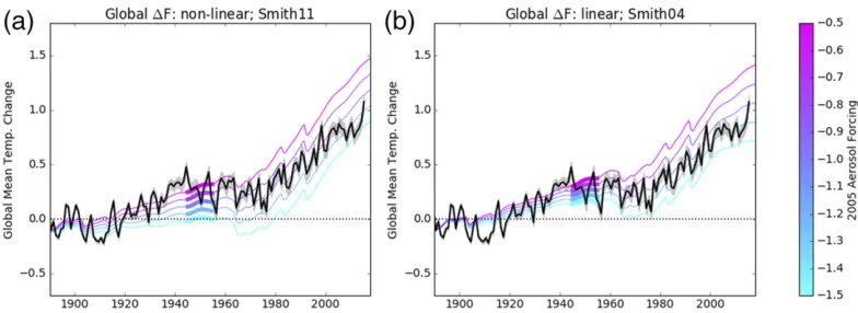
early that any nonlinear forcing response could be ac-counted for. However, if we were able to account for volcanic forcings (as we do here) and the global (if not regional) aerosol forcing responds linearly with past emissions changes (as in the discussion above of linear forcing) then there are no reasons to choose this over any other period. In the wider context of the twentieth century, the 1950s are unusual in that they tend to be consistent with lower estimates of aerosol forcing.Figure 2aprovides an illustration using a simple climate model [documented in Harris et al. (2013)] to translate forcing time series into global temperature changes, while keeping theSmith et al. (2011)emissions and nonlinear indirect aerosol represen-tation used in S15. This shows how varying the aerosol forcing (while fixing other parameters at their standard values) leads to a span of historical temperature changes. When theS15assumptions are retained, the simple model illustrates why 1950 suggests larger aerosol forcings are less consistent. Lower estimates of aerosol forcing are more consistent in early periods (present-day estimates on the order of 20.5 W m22 are more consistent in the 1950s); however, these tend to overestimate the warming in the later periods (when present-day aerosol forcings in the21.3 W m22ballpark are most consistent with 1990s temperatures). The reason why the simple model struggles to reproduce both early and late twentieth-century values is not clear. This could point to outlining combinations of climate sensitivity and heat uptake parameters required for a given aerosol forcing to match the whole record, or (as we go on to show) may instead relate to uncertain as-sumptions about historical aerosol emissions and how we

assume global aerosol forcing to be related to these. This wider twentieth-century context, however, suggests that caution is required before putting too much weight on a particular aerosol forcing period (such as the 1950s) as these forcing may not be reflective of the magnitude of aerosol changes required to reconcile later twentieth-century temperatures changes.

6. Outlook on the potential for requiring net positive 1950 energy balance to constrain the range of real-world aerosol forcing

TheS15constraint is attractive in that it provides a way to reduce present-day aerosol forcing uncertainty using simple and easily understood arguments. The central argument of our comment, however, is that this approach fails to cor-rectly predict a lack of forced trends in any CMIP5 models where aerosol forcing exceeds S15’s thresholds. Un-derstanding the cause of this inconsistency is not straight-forward, but we have identified several factors that may contribute. Stevens himself acknowledges that sensitivity to emissions and assumptions of linearity are likely to exist:

‘‘One advantage of the simple approach adopted here is that, even if one does not accept my arguments, they help identify what would be required for an aerosol forcing to be considerably more negative than about21.0 W m22. If, for instance, SO2emissions in 1950 relative to 1975 are

too large in the estimates bySmith et al. (2011), or if the forcing from aerosol–cloud interactions is for some rea-son linear in global SO2, a more negative aerosol forcing

becomes plausible’’ (p. 4811,S15).

FIG. 2. (a) The time series illustrating the dependence of global mean temperatures when varying on the mag-nitude of global 2005 aerosol forcing (denoted by the color bar) from an energy balance model/simple climate model [described inHarris et al. (2013)]. The temperatures in the 11 years centered around 1950 are highlighted by the thicker lines. The SO2emissions are taken fromSmith et al. (2011)and the indirect component of the global forcing is treated as logarithmic to these emissions (as perS15). The other simple model parameters are set at ‘‘central’’ values (climate sensitivity53 K; 23CO2radiative forcing53.71 W m22; land–sea contrast51.4; fraction of aerosol forcing treated as linear50.22; background natural emissions531.3). The mean (black) and uncertainty range (gray) for an observational estimate of historical temperature change fromMorice et al. (2012)

However, fromS15it was not evident what impact these choices would have on the constraint, which is what we have been able to estimate here. By changing either of these two factors [by assuming that the aerosol forcing responds linearly (globally if not locally) or by changing the SO2emissions toSmith et al. (2004)] we show that

the implied constraint changes from one that rules out aerosol forcing ranges simulated by the larger fraction of aerosol indirect effect capable CMIP5 simulations to a constraint that rules out none.

Concerns over the particular choice of time period aside, globally we see merits in exploring requirements for net forcing to be positive as a potential constraint. However, big questions need to be asked about such an approach that fails to predict the sign of forced tem-perature changes in CMIP5 models.Kretzschmar et al. (2017) have already used other inferences of CMIP5 historical aerosol forcing to highlight that the loga-rithmic global relationship of forcing with sulfur emis-sions used byS15 (and elsewhere) may be one factor behind this failure. In response Stevens and Fiedler (2017)identified behavior in the CMIP5 models, used in Kretzschmar et al. (2017), that questions the plausibility of these models’ historic forcing responses. However, it is difficult to assess to what extent the individual mod-eling errors identified imply that the logarithmic re-lationship employed inS15 would be a better model. BothStevens and Fiedler 2017andS15put forward data supporting this relationship but these forcing estimates cover only a handful of dates [only two inStevens and Fiedler (2017)and four inS15], none of which cover the 1900–75 period. This makes it difficult to have confi-dence in a logarithmic relationship, given that forcing estimates fromKretzschmar et al. (2017) and the new data presented in this comment highlight the potential for more linear global responses. Perhaps the best that can be said is thatS15and these subsequent comments highlight the need for more extensive time-evolving aerosol forcing estimates to better understand the line-arity of global forcing (or otherwise).

Moving beyond CMIP5, we have shown that the ap-plication of theS15constraint to the real world will be dependent on the historical sulfur emissions used. If the Smith et al. (2004)emissions are used instead and we assume forcing linearity, then the globalS15approach would not rule out any present-day aerosol forcings up to22.1 W m22(Fig. 1b).Figure 2bhelps illustrate why 1950’s temperature rise is less effective a constraint in this case. In contrast toFig. 2a,Fig. 2buses theSmith et al. (2004) emissions and assumes a globally linear aerosol forcing response to emissions. Consequently, global temperature changes estimated from a simple climate model are more similar up to the 1950s (Fig. 2b;

cf.Fig. 2a) and none of the simple climate model esti-mates fail to capture a warming trend. It is perhaps also worth noting that these assumptions make it easier to identify aerosol forcings that are consistent over the whole historical period. Mechanistically both factors [assuming linearity and using the Smith et al. (2004) emissions] lead to a smaller fraction of the present-day aerosol forcing being realized by 1950. The consequence is that net forcing or temperature change to 1950 is much less effective at discriminating amongst the present-day aerosol forcing estimates.

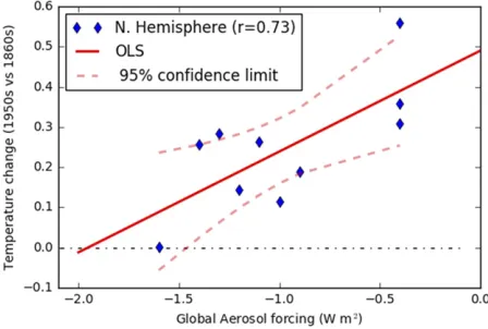
We findS15’s NH-only approach to be a more ques-tionable constraint. This is the constraint that enabled S15to rule out present-day aerosol forcings more neg-ative than 21.0 W m22. By linking the sign of hemi-spheric forcing to the sign of hemihemi-spheric temperature changeS15neglects the role of cross-equatorial energy flux, which we know to be important (see the discussion above of hemispheric constraints). However, CMIP5 models do suggest a fairly strong relationship between the magnitude of global forcing and the forced tem-perature trend to 1950 (r50.73), suggesting that it may be worth pursuing. The aerosol forcing explains roughly 50% of the CMIP5 spread in NH forced temperature trends (with presumably differences in other forcings, efficacy of climate sensitivity, and climate model errors also influencing this spread). If we regress the CMIP5 relationship between global present-day forcing and NH forced preindustrial to 1950 temperature change, we get a best estimate constraint of 22.0 W m22 (Fig. 3). Incidentally, if, as Stevens and Fiedler (2017) argue, there are good reasons to exclude GFDL-CM3, then the

FIG. 3. The relationship between present-day global aerosol forcing and the magnitude of forced (ensemble mean) temperature rise between the 1860s and 1950s from the CMIP5 models used in

implied constraint on aerosol forcings is weaker still. There is substantial uncertainty around this regressed re-lationship butS15’s21.0 W m22constraint is clearly not consistent with this (Fig. 3). This analysis suggests that there may be merit in pursuing hemispheric-only con-straints on aerosol forcing but that we do not have the right conceptual framework to do this at present (to account for factors like cross-equatorial energy transfer, for example). In summary, we conclude that global mean energy balance arguments put forward byS15imply an overly strong constraint that is inconsistent with what we see in current process-based climate models. Reevaluating the S15methodology constraint using different, but plausi-ble, assumptions, leads to weaker constraints on the magnitude of present-day aerosol forcing. Any real-world constraint would need to account for historical emission uncertainty and it is difficult to see how this could rule out aerosol forcings less negative than22.0 W m22, given the sensitivity to the underlying assumptions shown in this comment.

Acknowledgments. Ben Booth, Glen Harris, and Andy Jones were supported by the Met Office Hadley Centre Climate Programme funded by BEIS and Defra. Matt Hawcroft is supported by the Natural Environ-ment Research Council/DepartEnviron-ment for International Development via the Future Climates for Africa (FCFA) funded project ‘‘Improving Model Processes for African Climate’’ (IMPALA, NE/ M017265/1). Ken Carslaw was funded by the U.K. Natural Environment Research Council project ACID-PRUF (NE/I020148/1) with support from the Leeds–Met Office Academic Partnership (ASCI project).

REFERENCES

Carslaw, K. S., and Coauthors, 2013: Large contribution of natural aerosols to uncertainty in indirect forcing.Nature,503, 67–71,

https://doi.org/10.1038/nature12674.

Harris, G. R., D. M. Sexton, B. B. B. Booth, M. Collins, and J. M. Murphy, 2013: Probabilistic projections of transient climate change.Climate Dyn.,40, 2937–2972,https://doi.org/10.1007/ s00382-012-1647-y.

Hawcroft, M., J. M. Haywood, M. Collins, A. Jones, A. C. Jones, and G. Stephens, 2017: Southern Ocean albedo, inter-hemispheric energy transports and the double ITCZ: Global impacts of biases in a coupled model.Climate Dyn.,48, 2279–2295,https:// doi.org/10.1007/s00382-016-3205-5.

Haywood, J. M., and Coauthors, 2016: The impact of equilibrating hemispheric albedos on tropical performance in the HadGEM2-ES coupled climate model.Geophys. Res. Lett.,43, 395–403,

https://doi.org/10.1002/2015GL066903.

Kay, J. E., C. Wall, V. Yettella, B. Medeiros, C. Hannay, P. Caldwell, and C. Bitz, 2016: Global climate impacts of fixing the Southern Ocean shortwave radiation bias in the Community Earth Sys-tem Model (CESM).J. Climate,29, 4617–4636,https://doi.org/ 10.1175/JCLI-D-15-0358.1.

Kretzschmar, J., M. Salzmann, J. Mülmenstädt, O. Boucher, and J. Quaas, 2017: Comment on ‘‘Rethinking the lower bound on aerosol radiative forcing.’’J. Climate,30, 6579–6584,https:// doi.org/10.1175/JCLI-D-16-0668.1.

Loeb, N. G., H. Wang, A. Cheng, S. Kato, J. T. Fasullo, K. M. Xu, and R. P. Allan, 2016: Observational constraints on atmo-spheric and oceanic cross-equatorial heat transports: Re-visiting the precipitation asymmetry problem in climate models.Climate Dyn.,46, 3239–3257,https://doi.org/10.1007/ s00382-015-2766-z.

Mechoso, C. R., and Coauthors, 2016: Can reducing the incoming energy flux over the Southern Ocean in a CGCM improve its simulation of tropical climate?Geophys. Res. Lett.,43, 11 057– 11 063,https://doi.org/10.1002/2016GL071150.

Morice, C. P., J. J. Kennedy, N. A. Rayner, and P. D. Jones, 2012: Quantifying uncertainties in global and regional temperature change using an ensemble of observational estimates: The HadCRUT4 data set.J. Geophys. Res.,117, D08101,https:// doi.org/10.1029/2011JD017187.

Smith, S. J., R. Andres, E. Conception, and J. Lurz, 2004: Sulfur dioxide emissions: 1850–2000. Rep. PNNL-14537, 14 pp.,www. globalchange.umd.edu/data/publications/PNNL-14537.pdf. ——, J. van Aardenne, Z. Klimont, R. J. Andres, A. Volke, and

S. Delgado Arias, 2011: Anthropogenic sulfur dioxide emis-sions: 1850–2005.Atmos. Chem. Phys.,11, 1101–1116,https:// doi.org/10.5194/acp-11-1101-2011.

Stevens, B., 2015: Rethinking the lower bound on aerosol radiative forcing. J. Climate, 28, 4794–4819, https://doi.org/10.1175/ JCLI-D-14-00656.1.

——, and S. Fiedler, 2017: Reply to ‘‘Comment on ‘Rethinking the lower bound on aerosol radiative forcing.’’’J. Climate,30, 6585–6589,https://doi.org/10.1175/JCLI-D-17-0034.1. Twomey, S., and P. Squires, 1959: The influence of cloud