Quantifying quantum nonlocality

QUANTIFYING QUANTUM NONLOCALITY

Thesis by

Benjamin Francis Toner

In Partial Fulfillment of the Requirements for the Degree of

Doctor of Philosophy

California Institute of Technology Pasadena, California

2007

Copyright notice:

Chapter 2 is taken from [1], Chapter 4 is taken from [2], and Chapter 5 is taken from [3]. These works are copyrighted by the American Physical Society (APS), used with permission.

The remaining material is

to my parents,

Acknowledgements

First and foremost, I thank my advisor, John Preskill, for his guidance and support. The breadth of his knowledge has resulted in many insights, often in innocuous questions at the end of talks. I also owe thanks to Dave Bacon, who acted as a secondary advisor during my first years here at Caltech. I have been a teaching assistant for Alexei Kitaev and Jeff Kimble, and I have learned from them both.

John Preskill and Alexei Kitaev served on both my candidacy and thesis committees. I thank Jeff Kimble and Mark Wise, the other members of my candidacy committee, and Chris Umans and Alan Weinstein, the other members of my thesis committee.

Many people have been part of the Institute for Quantum Information during my time here. I thank Anura Abeyesinghe, Michael Adams, Charlene Ahn, Panos Aliferis, Robin Blume-Kohout, Sougato Bose, Sergey Bravyi, Andrew Childs, John Cortese, Sumit Daftuar, Andrew Doherty, Kovid Goyal, Sean Hallgren, Jim Harrington, Patrick Hayden, Hui Khoon Ng, Andrew Landahl, Debbie Leung, Hideo Mabuchi, Carlos Mochon, Ashwin Nayak, Michael Nielsen, Stefano Pironio, Ben Rahn, Robert Raussendorf, Leonard Schulman, Yaoyun Shi, Federico Spedalieri, Graeme Smith, Steven van Enk, Greg Ver Steeg, Frank Verstraete, Guifre Vidal, Pawel Wocjan, Jon Yard, and Michael Zwolak.

For administrative support I thank Donna Driscoll, Ann Harvey, and Carol Silberstein.

My parents, Mark and Chris, my siblings, Tim and Emily, and my good friend, Quynh-Nhu Nguyen, have been fantastic in encouraging me while overseas and I thank them for all they have done.

More specifically, I thank Antonio Ac´ın and Nicolas Gisin for encouraging Chapter 3 and for many helpful suggestions; John Preskill, Andrew Doherty, Patrick Hayden, Andre Methot, Carlos Mochon, and Michael Steiner for useful suggestions about Chapter 5; Richard Cleve, Michael Nielsen John Preskill, Graeme Smith, Frank Verstraete, and John Watrous for useful suggestions concerning Chapter 7; Richard Cleve and Wim van Dam for useful discussions about Chapter 8; and Steven Finch for providing me with Refs. [4, 5].

Joint work

Abstract

Quantum mechanics is nonlocal, meaning it cannot be described by any classical local hidden variable model. In this thesis we study two aspects of quantum nonlocality.

Part I addresses the question of what classical resources are required to simulate nonlocal quan-tum correlations. We start by constructing new local models for noisy entangled quanquan-tum states. These constructions exploit the connection between nonlocality and Grothendieck’s inequality, first noticed by Tsirelson. Next, we consider local models augmented by a limited amount of classical communication. After generalizing Bell inequalities to this setting, we show that (i) one bit of communication is sufficient to simulate the correlations of projective measurements on a maximally entangled state of two qubits, and (ii) five bits of communication are sufficient to simulate the joint correlation of two-outcome measurements on any bipartite quantum state. The latter result can be interpreted as a stronger (constrained) version of Grothendieck’s inequality.

Contents

Acknowledgements iv

Abstract vi

1 Introduction 1

1.1 Motivation . . . 1

1.2 Nonlocal correlations . . . 1

1.2.1 An example . . . 1

1.2.2 Notation and definitions . . . 3

1.2.3 Bell polytopes . . . 5

1.2.4 The CHSH inequality . . . 6

1.2.5 Measures of nonlocality . . . 8

1.3 Overview of the thesis . . . 10

1.3.1 Classical models for the quantum joint correlation . . . 10

1.3.2 Monogamy of nonlocal correlations . . . 11

I

Classical Models for the Quantum Joint Correlation

12

2.2 Werner states . . . 16

2.3 Generalization to higher dimensions . . . 18

2.4 Bell inequalities for Werner states . . . 20

2.5 Conclusions . . . 20

3 Local models for noisy entangled quantum states: constructions 21 3.1 Introduction . . . 21

3.2 A primitive for LHV models . . . 23

3.4 LHV model based on Krivine’s upper bound onK_G . . . 25

3.5 LHV model based on Krivine’s upper bound onKG(3) . . . 27

3.6 LHV model based on Krivine’s upper bound onK_G(n) . . . 31

3.7 LHV model based on Krivine’s upper bound onKG(2) . . . 34

3.8 Discussion . . . 38

4 Bell inequalities with auxiliary communication 40 4.1 Introduction . . . 40

4.2 The model . . . 41

4.3 Bell polytopes . . . 42

4.4 Bell inequalities with auxiliary communication . . . 43

4.4.1 Complete set of Bell inequalities with auxiliary communication . . . 44

4.4.2 Complete set of Bell inequalities for the joint observable . . . 45

4.5 Conclusion . . . 47

5 Communication cost of simulating Bell correlations 48 5.1 Introduction . . . 48

5.2 Simulation protocol . . . 49

5.3 Application to teleportation experiments . . . 53

5.4 Conclusion . . . 54

6 Communication cost of simulating the quantum joint correlation 55 6.1 Introduction . . . 55

6.2 A communication primitive . . . 55

6.3 Simulation of the joint correlation using five bits of communication . . . 56

6.4 Discussion . . . 58

II

Monogamy of Nonlocal Correlations

59

7.2 Framework . . . 61

7.2.1 The CHSH game . . . 61

7.3 Main technique . . . 62

7.4 Applications . . . 62

7.4.1 An analogue of the CKW theorem for nonlocal quantum correlations . . . 62

7.4.3 The odd cycle game . . . 64

8 Monogamy of nonlocal quantum correlations 69

8.1 Introduction . . . 69 8.2 Dimensional reduction . . . 70 8.3 Monogamy trade-off relation . . . 71

A Calculation of the constant c3 75

B Signs of the derivatives ofh(x) 77

Chapter 1

Introduction

1.1

Motivation

In 1935, Einstein, Podolsky, and Rosen suggested that quantum theory might emerge from a de-terministic local theory, by averaging over the values of somehidden variables, or properties of the system inaccessible to experiment [6]. Some thirty years later, Bell proved that this is impossible: Any hidden variable model for quantum theory must be nonlocal, in a manner I shall make precise be-low [7]. Bell’s conclusion has since been validated by a large number of experiments [8, 9, 10, 11, 12]. More recently, theoretical research into quantum algorithms [13], quantum communication com-plexity [14], and quantum cryptography [15] has shown that quantum devices are more powerful than their classical counterparts. Indeed, the goal of the burgeoning field of quantum information theory [16] is to obtain an information-theoretic understanding of the power of quantum resources. Here I apply this perspective to one quantum resource: nonlocal correlations. The aim is to go beyond the conclusion that quantum theory is nonlocal, instead answering the question of justhow nonlocal it is.

1.2

Nonlocal correlations

1.2.1

An example

We start with an example. Alice and Bob, who will star in this thesis, each have a machine. Each machine has a switch, which can be in one of two positions (labeled 0 and 1), together with two lights, a red one and a green one. Every second, exactly one of the lights flashes.

After running some experiments, Alice deduces the following:

1. No matter which position her switch is in, the red light will flash with probability 1/2, otherwise the green light will flash.

2. No matter which position his switch is in, the red light will flash with probability 1/2, otherwise the green light will flash.

But when they look at each other’s machines, they observe that

3. If Alice’s switch and Bob’s switch are both in position 1, then the color of Alice’s light is always different from the color of Bob’s light; otherwise their lights are always the same color. Furthermore, this is true no matter how far apart the machines are. So, although the colors of the lights on Alice and Bob’s machines are locally random, they are correlated in a way that depends on how their switches are set. After providing the relevant definitions, we’ll prove below that these correlations are nonlocal, meaning they are incompatible with any classical local theory. In fact, the machines just described are together known as a nonlocal box [17, 18]. We make three observations: 1. The switches are essential. Suppose the switches on Alice and Bob’s machines are stuck in position 1. Then Alice and Bob’s machines are just a correlated random source, a classical resource.

2. The machines can be realized with instantaneous communication and a correlated random source. Suppose that, by some means, the position of Alice’s switch is (instantaneously) com-municated to Bob’s machine. Then this is sufficient to reproduce their behavior. Of course, instantaneous communication is unphysical.

3. The machines cannot be used to communicate. Suppose Alice is in Amsterdam and Bob in Melbourne. Then there is no way for Alice to send a message to Bob using the machines. No matter how she sets her switch, the data Bob obtains from his machine is just a sequence of random bits. It is only when Alice and Bob meet up and compare their data that they notice something nonclassical is going on. We term such correlations no-signaling. No-signaling correlations are a weaker information-processing resource than communication, but a stronger resource than a classical correlated random source.

The operation of the machines can be summarized by specifying theconditional joint probability distribution of Alice and Bob’s results. Assume Alice sets her switch in positioni∈ {0,1} and Bob sets his in positionj∈ {0,1}. Label the output of Alice’s machine (the color of the light)a∈ {0,1},

and the output of Bob’s b ∈ {0,1}. Then the probability that Alice observes outcomea and Bob observes outcomebis

Pr(a, b|i, j) = 1

2[a⊕b=i∧j], (1.1)

where [t] = 1 if the clausetis true and 0 otherwise.

by the end of this chapter that the machine described above is unphysical: The distribution Eq. (1.1) is not realizable, even with quantum resources.

1.2.2

Notation and definitions

We restrict attention to scenarios with two parties, Alice and Bob. In ameasurement scenario, each party selects one ofM measurements (labeled 0,1, . . . , M−1) and then outputs one ofK different outcomes (labeled 0,1, . . . , K−1). Mostly we shall be interested in the caseK = 2. As above, we label Alice’s measurementi, and Bob’sj. Alice’s output is labeleda; Bob’s b.

A local hidden variable (LHV) model for a measurement scenario is defined as follows:

Definition 1.2.1 (LHV model). An LHV model for a (bipartite) measurement scenario is defined by (i) a set Λ and a probability distributionqover Λ, (ii) a functionA: Λ×Z_M →Z_K, and (iii) a functionB: Λ×Z_M →Z_K. We write the LHV model as a protocol:

Protocol 1.2.2. (Random Variables)Alice and Bob share a variableλ∈Λ, chosen according to the distributionq.

(Alice) Alice outputsa=A(λ, i).

(Bob)Bob outputsb=B(λ, j).

We note that this definition is completely general: Any unshared randomness can be replaced by shared randomness on which the one party does not act. To calculate the resulting conditional probability distribution, we average overλ:

Pr(a, b|i, j) =

dλ q(λ)[a=A(λ, i)][b=B(λ, j)]. (1.2)

If there exists an LHV model reproducing some correlationsp(a, b|i, j), we say that the correla-tions arelocal. Otherwise they arenonlocal.

Definition 1.2.3(No-signaling conditional probability distribution). A conditional probability dis-tribution is no-signaling if each party’s marginal disdis-tribution is independent of the other’s choice of input. More formally,p(a, b|i, j) is no-signaling if

Pr(a|i, j) =

b

p(a, b|i, j) (1.3)

is independent ofj for allaandiand

Pr(b|i, j) =

a

p(a, b|i, j) (1.4)

Nonlocal correlations in quantum theory arise from making local measurements on entangled quantum states. We assume that Alice and Bob share a mixed quantum state ρwith support on HA⊗ HB, whereHA (HB) is the local Hilbert space of Alice’s (Bob’s) system. The dimensions of the local spaces are denoteddA= dimHA,dB = dimHB. By extending the smaller of HAand HB we can assume that the local spaces have the same dimensiond= max(dA, dB). The operator11d is

the identity operator operating on a space of dimensiond. Where it is clear from the context, we omit the subscript indicating the dimension. The most general measurement possible in quantum theory is termed a postive operator-valued measure (POVM). A K-outcome POVMM on HA is

defined byK positive Hermitian operatorsA₀,A₁, . . . ,A_K−1 such that_kA_k =11. The elements

A_k are termedeffects.

Definition 1.2.4 (quantum model). A quantum model for a (bipartite) measurement scenario is defined by (i) a stateρonHA⊗ HB; (ii) a set ofM POVMsMionHA with effectsAai; and (iii) a

set ofM POVMs Nj onHB with effectsBbj. We write the quantum model as a protocol:

Protocol 1.2.5. (Preparation) Alice and Bob share the stateρ.

(Alice)Alice measures the POVMMi onρ, outputting her resulta.

(Bob)Bob measures the POVMNj onρ, outputting his resultb.

This results in the conditional probability distribution

Pr(a, b|i, j) = trA_ia⊗Bb_jρ. (1.5) We say that a conditional probability distributionp(a, b|i, j) isrealizable with quantum resourcesif there is a quantum model forp(a, b|i, j).

Specializing to two-outcome measurements, we define thejoint correlation

αiβj =

1

a,b=0

(−1)a+b_{Pr(a, b|i, j). (1.6)}

We define theobservablecorresponding to a two-outcome measurementMasA=A0−A1. When Alice measures an observableAonρ, we label the outcomeα∈ {−1,+1}. We similarly label Bob’s

outcomeβ. Denote the set of possible observables byO_Afor Alice andO_B for Bob. Then the joint correlation of Alice and Bob’s measurement results is given by

αβ QM= tr (A⊗Bρ). (1.7)

marginal probabilitiesare given by

αQM = tr (A⊗11Bρ), (1.8)

β _QM = tr (11A⊗Bρ). (1.9)

Together, these three equations define the full probability distribution for two-outcome measure-ments onρ.

Often the conditional probability distributions we wish to study arise from making measure-ments on quantum states, in which case the existence of a quantum model is trivial. A quantum measurement scenariofor two-outcome measurements is a measurement scenario where we label the measurements by the corresponding quantum observables. For completeness, we state the following:

Definition 1.2.6 (LHV model for two-outcome observables). An LHV model for a (bipartite) quantum measurement scenario is defined by (i) a set Λ and a probability distributionqover Λ, (ii) a functionA: Λ× OA→ {−1,+1}, and (iii) a functionB: Λ× OB→ {−1,+1}. We write the LHV

model as a protocol:

Protocol 1.2.7. (Random Variables)Alice and Bob share a variableλ∈Λ, chosen according to the distributionq.

(Alice)Alice outputsa=A(λ,A).

(Bob)Bob outputsb=B(λ,B).

We average over λto calculate the resulting correlations:

α_LHV =

dλ q(λ)A(λ,A), (1.10)

β _LHV =

dλ q(λ)B(λ,B), (1.11)

αβ LHV =

dλ q(λ)A(λ,A)B(λ,B). (1.12)

We say that the LHV model reproduces the joint correlation on a stateρwhenαβ _LHV=αβ _QM

for all observablesAandB. We say that the LHV model reproduces the full probability distribution when, in addition,α LHV=α QM andβ LHV=β QM.

1.2.3

Bell polytopes

Consider a deterministic protocol, i.e., one in which no randomness, shared or otherwise, is used. Each party’s output can only depend on their local measurement. Such a protocol is characterized by the two functionsA and B in Def. 1.2.1, which describe the outcomes of the two parties’ mea-surements: IfAselects measurementi, she outputsA(i) and ifBselects measurementj, he outputs

B(j). The probabilities for the scenario are thenp(a, b|i, j) = [a=A(i)][b=B(j)].

By listing the components, we may view the probabilities p(a, b|i, j) as vectors p in RD _with

D=M2(K2−1) (there is a normalization constraint_a,bp(a, b|i, j) = 1). To each pair of functions {A, B}, there corresponds a deterministic protocol, so the set of all deterministic protocols is a finite

collection of such vectors{dζ|ζ= 1, ..., K2M}.

Now consider the effect of allowing randomness. For any fixed choice of the random variables

λ∈ Λ, the functions A(λ,·) and B(λ,·) are deterministic, so that the set of all possible protocols

that use randomness is described by a convex sum of the deterministic protocols

p=

ζ

λζdζ,

ζ

λζ = 1, λζ ≥0. (1.13)

The set of all protocols therefore corresponds to a region ΩMK in RD, which is a polytope because

there is a finite number of extreme vectorsdζ [20]. This permits an alternative description: Instead

of describing the polytope ΩMK as the convex combination of a finite set of extreme points, we can

describe it by specifying a complete (finite) set of facet inequalities. A facet inequality is a pair {_{f , c }that defines a half-space ofR}D _{via the inequalityf·p≤c. Complete sets of facet inequalities}

f_η, c_η are satisfied if and only ifpis in Ω_MK:

p∈ΩMK iff fη·p≤cη, ∀η. (1.14)

Each facet is therefore a Bell inequality and complete sets of facet inequalities are complete sets of Bell inequalities. Complete sets are known in the two-party case when M = 2, K = 2 [21];

M = 3, K= 2;M = 2, K= 3 [22, 23]; and also when extra symmetry constraints are imposed [24].

1.2.4

The CHSH inequality

In the simplest nontrivial case M = 2, K = 2, there is (up to symmetries) one nontrivial Bell inequality, the Clauser-Horne-Shimony-Holt (CHSH) inequality [25]. Given a conditional probability distributionp(a, b|i, j), define

BCHSH(p) =α0β0 +α0β1 +α1β0 − α1β1 , (1.15)

Theorem 1.2.8([21, 25]). Suppose there is an LHV model for a distributionp(a, b|i, j). Then

BCHSH(p) ≤2. (1.16)

Furthermore, if a distribution p(a, b|i, j) satisfies Eq. (1.16), as well as equivalent inequalities ob-tained by permuting parties, measurements, and outputs, then it is obob-tained from some LHV model.

Proof. The proof of completeness is via facet enumeration, as described in the previous section, and we omit it. It is, however, simple to see that if there is an LHV model forp(a, b|i, j), then it satisfies the inequality. Suppose the LHV model is defined by a set Λ, a probability distributionqon Λ, and functionsA, B: Λ× {0,1} → {−1,+1}, where

αiβj =

dλq(λ)A(λ, i)B(λ, j). (1.17)

Then

BCHSH(p) =

dλq(λ) [A(λ,0) (B(λ,0) +B(λ,1)) +A(λ,1) (B(λ,0)−B(λ,1))] (1.18) ≤

dλq(λ) [|B(λ,0) +B(λ,1)|+|B(λ,0)−B(λ,1)|]. (1.19)

Now,|B(λ,0) +B(λ,1)|is either 0 or 2. If it is 0, we’re done; if it is 2, then|B(λ,0)−B(λ,1)|= 0. In either caseBCHSH(p) ≤2.

At this point we can return to the nonlocal box, the example of nonlocal correlations given at the start of this introduction. By construction, the correlations defined in Eq. (1.1),

Pr(a, b|i, j) = 1

2[a⊕b=i∧j], (1.20)

yieldα₀β₀ =α₀β₁ =α₁β₀ =−α₁β₁ = 1, which givesB_CHSH = 4. Since 4 is larger than 2, these correlations violate the CHSH inequality and are nonlocal. Furthermore, they are maximally nonlocal, within this measurement scenario.

The nonlocal box is a powerful resource. Consider some Boolean functionf :{0,1}n× {0,1}n→

{0,1}with twon-bit strings as inputs, labeledaandb. Alice knows stringa, while Bob knows string

The nonlocal box is not realizable with quantum resources. This follows from the following, due to Tsirelson:

Theorem 1.2.9(Tsirelson [28]). Suppose Alice and Bob make local measurements on an entangled quantum state, yielding a distributionp(a, b|i, j). Then

BCHSH(p) ≤2√2. (1.21)

Proof. Assume there is a quantum model forp(a, b|i, j). By taking a purification of the shared state

ρand conditioning on the randomness, it is sufficient to consider the case where Alice and Bob share a pure state|ψ . Suppose Alice measuresA_i on inputi, and BobB_j on inputj. Then

αiβj =ψ|Ai⊗Bj|ψ . (1.22)

Define|a_i =A_i⊗11_B|ψ and|b_j =11_A⊗B_j|ψ . Thena_i|a_i =b_j|b_j ≤1, since the eigenvalues ofA_i andB_j are in [−1,+1]. This implies

BCHSH(p) = a0|(|b0 +|b1 ) +a1|(|b0 − |b1 ) (1.23) ≤ |b₀ +|b₁ +|b₀ − |b₁ (1.24)

= 2 (cosθ/2 + sinθ/2) (1.25)

≤ 2√2, (1.26)

where cosθ=|b₀|b₁ |.

1.2.5

Measures of nonlocality

One benefit of narrowing in on one aspect of quantum theory—nonlocality—is that it allows us to compare quantum theory to stronger theories, and not just to classical mechanics. But first we need some way of measuring the nonlocality of some distributionp(a, b|i, j). We have seen one way already: the extent of violation of a Bell inequality. This measure is the right one in a number of contexts, such as the extent to which sharing entanglement allows the provers in a multi-prover interactive proof system to “cheat,” an application I have explored in Ref. [29]. But other measures are more relevant in physical applications, such as experimental tests of Bell inequality violation. We explore some of these here.

Resistance to noise—Given a distributionp(a, b|i, j), define the noisy distribution

where 0 ≤μ ≤1 and q(a, b|i, j) is a local distribution. What is the largest value of μ such that

p_μ(a, b|i, j) is local? Here the local distribution q(a, b|i, j) can be some fixed distribution, such as the uniform distribution, or can be chosen adversarily. We shall explore this measure in Chapters 2 and 3.

Communication cost of simulation—What is the communication complexity of generating a dis-tributionp(a, b|i, j)? In other words, suppose we augment an LHV model with a limited amount of communication, after the parties decide on which setting to measure and before they output results. How many bits of communication are required to reproduce the correlations exactly or approxi-mately? We formalize this notion for one-way communication (which is what will be relevant for our results) as follows:

Definition 1.2.10 (LHV model with cbits of one-way classical communication). An LHV model augmented by c bits of one-way classical communication for a (bipartite) measurement scenario is defined by (i) a set Λ and a probability distributionqover Λ, (ii) a functionA: Λ×Z_M →Z_K, (iii) a functionm: Λ×Z_M →Z_c, and (iv) a functionB: Λ×Z_M ×Z_c →Z_K. We write the model as a protocol:

Protocol 1.2.11. (Random Variables)Alice and Bob share a variableλ∈Λ, chosen according to the distributionq.

(Alice)Alice outputsa=A(λ, i). Alice sends a messagem=m(λ, i) to Bob.

(Bob)Bob outputsb=B(λ, j, m(λ, i)).

We explore this measure in Chapters 4, 5, and 6.

Dectector efficiency required for loophole-free Bell inequality violation—There are a number of “loopholes” in experimental tests of Bell inequality violation that a local theory might exploit in order to simulate quantum correlations. For example, if there is time for a signal to travel from Alice’s apparatus to Bob’s apparatus after she chooses her measurement but before he outputs his results, then it is possible to simulate what appear to be quantum correlations with classical resources. Known as the locality loophole, this can be closed by ensuring Alice and Bob’s measurement events are spacelike separated. This has been done experimentally in Refs. [9, 10, 11].

Statistical distance to local theories—How many trials of a Bell inequality experiment should we perform to observe a contradiction with LHV models at some level of statistical significance? In this case, the relevant parameter is the relative entropy between the nonlocal distribution and the best local model. See Ref. [30].

1.3

Overview of the thesis

1.3.1

Classical models for the quantum joint correlation

In the first part of the thesis, we study classical models for the joint correlationαβ _QM= tr (A⊗Bρ), resulting from performing two-outcome measurements on a quantum stateρ.

For a quantum stateρ, define

ρμ=μ ρ+ (1−μ)

11

dAdB

. (1.28)

In Chapter 2 we give bounds on the amount of noise required to make the correlations onρ_μ local. These build on work of Tsirelson [31, 32], who connected Bell inequality violation with Grothendieck’s inequality. For two-qubit Werner states ρW

μ =μ|ψ− ψ−|+ (1−μ)11/4, we show that there is an

LHV model for projective measurements if and only if μ≤1/KG(3). If we restrict the projective

measurements to a plane, then there is a local model for projective meausurements onρμif and only

ifμ≤1/√2.

In Chapter 3, we exploit this connection to construct explicit LHV models, based on (the proofs of) Krivine’s upper bounds on K_G(n) [33]. Among the constructions are local hidden variables models for (i) projective measurements on the qubit-qubit Werner state ρW

μ = μ|ψ− ψ−|+ (1−

μ)11/4, forμ≤0.6595, (ii) the joint correlation of projective measurements onρμ=μ ρ+ (1−μ)11/4,

where ρis an arbitrary qubit-qubit quantum state, forμ≤0.6009; and (iii) traceless two-outcome observables on ρmax_μ =μ|ψ_d+ ψ_d+|+ (1−μ)11/d2, where |ψ+_d is a maximally entangled state in d

dimensions, forμ≤0.5611.

Next we turn to simulation with LHV models augmented by classical communication. In Chap-ter 4, we show how to generalize Bell inequalities to this setting. Suppose Alice and Bob each choose one of M two-outcome measurements and exchange one bit of information. We present the complete set of inequalities forM = 2, and the complete set of inequalities for the joint correlation observable forM = 3. The correlations produced by quantum theory satisfy both of these sets of inequalities. One bit of communication is therefore sufficient to simulate quantum correlations in both of these scenarios.

show that certain quantum teleportation experiments, which teleport a single qubit, admit an LHV model.

Part I culminates in Chapter 6. Here we put the ideas of Chapters 2 and 3 together with those of Chapter 5 to show that five bits of communication are sufficient to simulate the joint correlation of two-outcome measurements on any bipartite quantum state. This result can be interpreted as a stronger (constrained) version of Grothendieck’s inequality.

1.3.2

Monogamy of nonlocal correlations

In Part II, we describe new techniques for obtaining Tsirelson bounds, or upper bounds on the quantum value of a Bell inequality. Since quantum correlations do not allow signaling, we obtain a Tsirelson bound by maximizing over all no-signaling probability distributions. In Chapter 7 we show this maximization can be cast as a linear program.

Part I

Classical Models for the Quantum

Chapter 2

Local models for noisy entangled

quantum states: existence

2.1

Introduction

In this chapter, we relate the nonlocal properties of noisy entangled states to Grothendieck’s constant, a mathematical constant appearing in Banach space theory. For two-qubit Werner states ρW

p =

p|ψ− ψ−|+ (1−p)11/4, we show that there is a local model for projective measurements if and only ifp≤1/KG(3), whereKG(3) is Grothendieck’s constant of order 3. Known bounds onKG(3) prove

the existence of this model at least forp0.66, quite close to the current region of Bell violation,

p∼0.71. We generalize this result to two-outcome measurements on arbitrary quantum states. This chapter is joint work with Antonio Ac´ın and Nicolas Gisin.

From an operational point of view it is not difficult to define when a quantum state exhibits nonclassical correlations. Suppose that two parties, Alice (A) and Bob (B), share a mixed quantum stateρwith support on H_A⊗ H_B, where H_A (H_B) is the local Hilbert space of A’s (B’s) system. Thenρ contains quantum correlations when its preparation requires a nonlocal quantum resource. Conversely, a quantum state is classically correlated, or separable, when it can be prepared using only local quantum operations and classical communication (LOCC). From this definition, due to Werner [34], it follows that a quantum state ρ is separable if it can be expressed as a mixture of product states, ρ = N_i=1pi|ψAi ψiA| ⊗ |ψBi ψBi |. A state that cannot be written in this form

has quantum correlations and is termed entangled. But the above definition, in spite of its clear physical meaning, is somewhat impractical. Tests to distinguish separable from entangled states are complicated [35], except whend_A = 2 andd_B ≤3 [36, 37], d_A andd_B denoting the dimensions of the local subsystems.

p

3

1

2

1

2

1

66

.

0

12

5

Separability Barrett's model[9] Werner's model[5]

This work CHSH violation

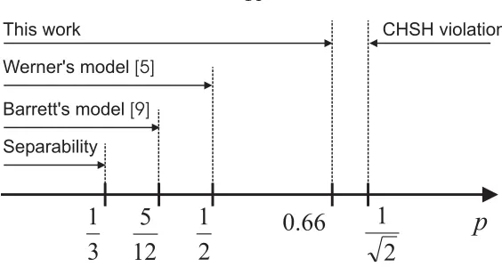
Figure 2.1: Nonlocal properties of two-qubit Werner states,ρW

p . Werner’s local model works up to

p= 1/2, while the CHSH inequality is violated whenp >2−1/2_{∼0.71. Here, we prove the existence}

of a local model for projective measurements whenp0.66.

yes [39]: All entangled pure states violate the CHSH inequality. In 1989, Werner showed that the previous result cannot be generalized to mixed states. He introduced what are now called Werner states, and gave a local hidden variable (LHV) model for measurement outcomes for some entangled states in this family [34]. Although the construction only worked for projective measurements, his result has since been extended to general measurements [40].

In spite of these partial results, it is generally extremely difficult to determine whether an entan-gled state has a local model or not, since (i) finding all Bell inequalities is a computationally hard problem [22, 41] and (ii) the number of possible measurement is unbounded (see however [42] for recent progress). This question remains unanswered even in the simplest case of Werner states of two qubits. These are mixtures of the singlet|ψ− = (|01 − |10 )/√2 with white noise of the form

ρW_p =p|ψ− ψ−|+ (1−p)11

4. (2.1)

It is known that Werner states are separable iffp≤1/3, admit an LHV model for all measurements for p≤5/12 [40], admit an LHV model for projective measurements for p≤1/2 [34] and violate the CHSH inequality for p > 1/√2 (see Fig. 2.1). However, the critical value of p, denoted pW

c ,

at which two-qubit Werner states cease to be nonlocal under projective measurements is unknown. This question is particularly relevant from an experimental point of view, since pW_c specifies the amount of noise the singlet tolerates before losing its nonlocal properties.

In this chapter, we exploit the connection between correlation Bell inequalities and Grothendieck’s constant [43], first noticed by Tsirelson [31], to prove the existence of a local model for several noisy entangled states. We first demonstrate thatpW

c is related to a generalization of this constant, namely,

pW

c = 1/KG(3), whereKG(3) is Grothendieck’s constant of order 3 [33]. The exact value ofKG(3)

is unknown, but known bounds establish that 0.6595 ≤ pW c ≤ 1/

√

(see Fig. 2.1). Next, we show that if Alice (or Bob) is restricted to make measurements in a plane of the Poincar´e sphere, then there is an explicit LHV model for all p ≤ 1/K_G(2) = 1/√2. This improves on the bound of Larsson, who constructed an LHV model for planar measurements for

p≤2/π[44]. Thus, in the case of planar projective measurements, violation of the CHSH inequality completely characterizes the nonlocality of two-qubit Werner states.

In the case oftraceless two-outcome observables, we can extend our results to mixtures of an arbitrary stateρonCd_⊗Cd_{with the identity, of the form}

ρ_p=p ρ+ (1−p)11

d2. (2.2)

Denote bypc(ρ) the maximum value ofpfor which there exists an LHV model for the joint correlation

of traceless two-outcome observables onρp, and define

pd_c = min

ρ pc(ρ) pc= limd→∞p d

c. (2.3)

Thenpc= 1/KG where KG is Grothendieck’s constant. Again, the exact value ofKG is unknown,

but known bounds imply 0.5611≤pc≤0.5963.

Finally, we discuss the opposite question of finding Bell inequalities better than the CHSH inequality at detecting the nonlocality ofρW

p , or, more generally, of Bell diagonal states.

Before proving our results, we require some notation. We write a two-outcome measurement by Alice as{A+, A−}, where the projectorsA± correspond to measurement outcomes±1. Similarly, a two-outcome measurement made by Bob is denoted{B+, B−}. We define theobservable correspond-ing to Alice’s (Bob’s) measurement asA=A+−A− (B=B+−B−). An observableAistraceless if trA = 0, or equivalently trA− = trA+. The joint correlationof Alice and Bob’s measurement results, denotedαandβ, respectively, is

αβ = tr (A⊗B ρ). (2.4)

Alice’slocal marginal is specified byα = tr (A⊗11ρ), and Bob’s byβ = tr (11⊗B ρ). Together, αβ , α andβ define the full probability distribution for two-outcome measurements onρ. An LHV model for the full probability distribution is one that gives the same valuesαβ ,α andβ as quantum theory. An LHV model for the joint correlation is one that gives the same joint correlation αβ , but not necessarily the correct marginals. In the qubit case, the projective measurements

2.2

Werner states

Let us first consider the case of Werner states (2.1). For projective measurements on ρW p , LHV

simulation of the joint correlation is sufficient to reproduce the full probability distribution. This follows from:

Lemma 2.2.1. Suppose that there is an LHV model L that gives joint correlation αβ L. Then

there is an LHV modelL with the same joint correlation and uniform marginals: αβ _L =αβ _L, α_L =β _L = 0.

Proof. Let α and β be the outputs generated by the LHV L (dependent on the hidden variables and measurement choices). Define a new LHVL by augmenting the hidden variables ofLwith an additional random bitc∈ {−1,1}. InL, Alice outputscαand Bob cβ.

Therefore, the analysis of the nonlocal properties of Werner states under projective measurements can be restricted to Bell inequalities involving only the joint correlation. Actually, this holds for any Bell diagonal state, under projective measurements, since trAρ= trBρ=11/2 for all these states,

so all projective measurements give uniform marginals. In the Bell scenarios we consider, Alice and Bob each choose frommobservables, specified by{A1, . . . , Am}and{B1, . . . , Bm}. We can write a

generic correlation Bell inequality as

|

m

i,j=1

M_ijα_iβ_j | ≤1, (2.5)

where M = (M_ij) is anm×m matrix of real coefficients defining the Bell inequality. The matrix

M is normalized such that the local bound is achieved by a deterministic local model, i.e.,

max

ai=±1, bj=±1|

m

i,j=1

Mijaibj|= 1. (2.6)

For the singlet stateα_iβ_{j Ψ}−=−a_i·b_j. We obtain the maximum ratio of Bell inequality violation for the singlet state, denoted Q, by maximizing over normalized Bell inequalities, and taking the limit as the number of settings goes to infinity:

Q= lim

m→∞sup_Mij max_ai,bj| m

i,j=1

Mijai·bj|. (2.7)

Since all joint correlations vanish for the maximally mixed state, it follows that the critical point at which two-qubit Werner states do not violate any Bell inequality ispW

c = 1/Q.

details). Grothendieck’s inequality first arose in Banach space theory, particularly in the theory of p-summing operators [45]. We shall need a refinement of his constant, which can be defined as follows [43]:

Definition 2.2.2 (Grothendieck’s constant of order n). For any integer n ≥ 2, Grothendieck’s constant of ordern, denotedKG(n), is the smallest number with the following property: LetM be

anym×mmatrix for which

|

m

i,j=1

Mijaibj| ≤1, (2.8)

for all real numbersa₁, . . . , am, b1, . . . , bm∈[−1,+1]. Then

|

m

i,j=1

M_ija_i·b_j| ≤K_G(n), (2.9) for all unit vectorsa₁, . . . , am,b1, . . . ,bminRn.

Definition 2.2.3(Grothendieck’s constant). Grothendieck’s constant is defined as

K_G= lim

n→∞KG(n). (2.10)

The best bounds currently known for KG are 1.6770≤KG ≤π/(2 log(1 +

√

2)) = 1.7822 [46]. The lower bound is due to Reeds and, independently, Davies [4, 5], while the upper bound is due to Krivine [33].

It follows immediately from the first definition that the maximal Bell violation for the singlet state (2.7) isKG(3). We have therefore proved

Theorem 2.2.4. There is an LHV model for projective measurements on the Werner state ρW p if

and only ifp≤pW_c = 1/KG(3).

It is known that√2≤KG(3)≤1.5163. The lower bound follows from the CHSH inequality; the

upper bound is again due to Krivine [33]. He shows thatK_G(3)≤π/(2c₃) where c₃ is the unique

solution of _√

c₃

2

_c3

0 t

−3/2_{sint dt= 1 (2.11)}

in the interval [0, π/2]. Numerically we find that c3 ≈1.0360. This implies KG(3) ≤1.5163 and

pW_c ≥0.6595. Furthermore, it turns out that an explicit LHV model emerges from Krivine’s upper bound onK_G(3), as we shall see in the following chapter.

Another result follows from Krivine’s work:

Theorem 2.2.5. If Alice’s projective measurements are restricted to a plane in the Poincar´e sphere, then there is an LHV model for ρW

p if and only if p≤1/

Proof. In this case, the vectors a_i in (2.7) are two-dimensional. Since the quantum correlation depends only on the projection ofb_j ontoa_i, we can assume that the vectorsb_j lie in the same plane. It follows thatpW

c = 1/KG(2) for planar measurements, and Krivine has shown thatKG(2)

is equal to√2 [33].

Again Krivine’s proof can be adapted to give an explicit LHV model for planar measurements, valid forp≤1/√2 and we shall do this in the next chapter.

2.3

Generalization to higher dimensions

It is possible to extend these results to general states of the form (2.2), if we restrict our analysis to correlation Bell inequalities oftracelesstwo-outcome observables. Admittedly, this analysis is far from sufficient. Indeed, it does not allow us to determine whether the full probability distribution admits an LHV model even in the case of two-outcome measurements, since the most general Bell inequalities have terms that depend on marginal probabilities [23]. Mindful of this caveat, we now prove the existence of LHV models for the joint correlation of the states (2.2). To make the connection with Grothendieck’s constant, we start with a representation of quantum correlations as dot products, first noted by Tsirelson [31]. It is sufficient to restrict to the case of pure states, since we can obtain an LHV model for a mixed stateρby decomposing it into a convex sum of pure states, and taking a convex combination of the LHVs for those pure states.

Lemma 2.3.1. Suppose Alice and Bob measure observables A and B on a pure quantum state |ψ ∈ Cd_⊗Cd_{. Then we can associate a real unit vectora∈R}2d2 _{with A (independent of B), and}

a real unit vectorb∈R2d2 _{with B (independent ofA) such that αβ}

ψ =a·b. Moreover, if |ψ is

maximally entangled, then we can assume the vectorsaandblie inRd2−1_.

Proof. Let|a =A⊗11B|ψ and|b =11A⊗B|ψ . Thenαβ =a|b ,a|a =b|b = 1. Denote the

components of|a asaiwherei= 1,2, . . . , d2, and similarly for|b . We now define a 2d2–dimensional

real vectora= (Rea1, Ima1, Rea2, Ima2, . . . , Read2, Ima_d2), and similarlyb= (Reb₁, Imb₁, Reb₂,

Imb₂, . . . , Reb_d2, Imb_d2). Thena·a=b·b= 1 andαβ =a·b(because a|b is real).

If |ψ is maximally entangled, we can assume |ψ = |ψ+ = 1/√dd_i=1|ii . We calculate αβ _ψ+ = tr_A(ABt)/d where Btis the transpose ofB. Introduce a (d2−1)–dimensional basis g_i

for traceless operators onH_A, normalized such that tr (g_ig_j) =dδ_ij. LetA=_ia_ig_i,Bt₌ ibigi,

which define the vectorsa andb. Squaring these definitions and taking the trace gives _ia2_i =

ib2i = 1. Finally, tr (ABt) =d

iaibj, which implies thatαβ =

iaibi=a·b.

The converse of Lemma 2.3.1 is also true: All dot products of normalized vectors,a,b∈Rn_{, are}

Ref. [31]. For the sake of completeness, we state it here without proof (see [31] for the details).

Theorem 2.3.2 (Tsirelson [31]). Let {ˆai}mi=1 and {ˆbj}mj=1 be sets of unit vectors in Rn. Let d=

2n/2 and |Φ be a maximally entangled state onCd⊗Cd. Then there are observables A1. . . , Am

andB₁. . . , B_m onCd _{such that}

αi = Φ|Ai⊗11|Φ = 0, (2.12)

β_j = Φ|11⊗B_j|Φ = 0, (2.13)

αiβj = Φ|Ai⊗Bj|Φ = ˆai·ˆbj, (2.14)

for all1≤i, j≤m.

Note that in our case, the stipulation that the observables be traceless ensures that their out-comes are random on the maximally mixed state. Theorem 2.3.3 follows from Lemma 2.3.1 and Theorem 2.3.2:

Theorem 2.3.3. Letρbe a state on Cd_⊗Cd _{and define ρ}

p andpdc as in Eqs. (2.2,2.3). Then

1

KG(2d2) ≤

pd_c ≤ 1

KG(2log2d+ 1). (2.15)

In other words, there is always an LHV model for the joint correlation of traceless two-outcome observables onρpforp≤1/KG(2d2) and there is a state (in fact, the maximally entangled state on

log₂dqubits) such that the joint correlation is nonlocal forp >1/KG(2log2d+ 1).

Corollary 2.3.4. The threshold noise for the joint correlation of two-outcome traceless observables isp_c= 1/K_G.

This follows from the previous theorem, taking the limit d → ∞. The known bounds imply

0.5611≤pc ≤0.5963. Compare this tops, the threshold noise at which the stateρp is guaranteed

separable: Whilep_s decreases with dimension at least as 1/(1 +d) [47],p_c approaches a constant. In the case of two-qubit systems, we can be more specific, because projective measurements are traceless and have two outcomes:

Corollary 2.3.5. Supposeρis an arbitrary state onC2⊗C2. Then there is an LHV model for the joint correlation on ρ_p =p ρ+ (1−p)11/4 for p≤1/K_G(8). In particular, K_G(8) ≤1.6641 [33], which implies there is an LHV model forp≤0.6009.

For maximally entangled states, marginals of traceless observables are uniform, so Lemmas 2.2.1 and 2.3.1 imply:

Cd_⊗Cd_{. Then there is an LHV for the full probability distribution arising from traceless observables}

for p≤1/K_G(d2−1).

2.4

Bell inequalities for Werner states

Just as upper bounds onKG(n) yield LHV models, lower bounds yield Bell inequalities. The case of

Werner states appears of particular interest: At present, there is no Bell inequality better than CHSH at detecting the nonlocality ofρW_p . This and other approaches to construct new Bell inequalities will be presented in [48]. Unfortunately, none of these inequalities could be proven to be better than CHSH. It is remarkable how difficult it is to enlarge this region of Bell violation or, equivalently, to show thatK_G(3)> K_G(2) =√2. Actually, in the case of random marginal probabilities, as for Bell diagonal states under projective measurements, no improvement over the CHSH inequality can be obtained using 3×nmeasurements [49].

This result, however, would imply that KG(3) =KG(2) =

√

2, which seems unlikely. Actually, one can find in [46] an explicit construction with 20 settings showing that KG(5) ≥ 10/7 >

√ 2. More recently, one of us has shown thatKG(4)>

√

2 as well [48].

2.5

Conclusions

Chapter 3

Local models for noisy entangled

quantum states: constructions

3.1

Introduction

In the preceding chapter, I, with Ac´ın and Gisin, related the nonlocal properties of noisy entangled states to K_G(n), Grothendieck’s constant of order n. In this chapter, I exploit this connection to construct explicit local hidden variables models, based on Krivine’s proofs of upper bounds on

KG(n).

As before, we consider the one-parameter family of states obtained by mixing an arbitrary quan-tum stateρwith white noise

ρp=p ρ+ (1−p)11d/d2, (3.1)

where 0≤p≤1. We list our results:

1. Qubit-qubit Werner states are mixtures of the singlet|ψ− = (|01 −|10 )/√2 with white noise of the form

ρW_p =p|ψ− ψ−|+ (1−p)11

4. (3.2)

It is known that Werner states are separable iffp≤1/3, admit an LHV model for all measure-ments forp≤5/12 [40], admit an LHV model for projective measurements forp≤1/2 [34] and violate the CHSH inequality forp >1/√2 (see Fig. 2.1). In the previous chapter, we showed that there is an LHV model for projective measurements iffp≤1/KG(3). AlthoughKG(3) is

not known exactly, it is known that√2≤KG(3)≤1.5163. The lower bound comes from the

CHSH inequality; the upper bound is due to Krivine [33]. He shows that KG(3) ≤π/(2c3)

where c3 is the unique solution of √

c₃

2

c3

0 t

in the interval c₃ ∈ [0, π/2]. Numerically we find that c₃ ≈ 1.0360. This implies K_G(3) ≤ 1.5163. It turns out that we can extract an explicit LHV model from Krivine’s proof, valid for

p≤0.6595. We present it in Section 3.5. 2. For projective measurements onρW

p , but where Alice’s measurements are restricted to a plane

of the Poincar´e sphere, there is an LHV model iff p ≤ 1/KG(2) = 1/

√

2. We construct this model in Section 3.7. Previously, it was known that there is an LHV model for planar measurements forp≤2/π= 0.6366 [44].

3. For the joint correlation of projective meausurements onpρ+(1−p)11/4, whereρis an arbitrary state on C2⊗C2, there is an LHV model for p≤1/KG(8). Known bounds give an explicit

model for p≤0.6009. We give this construction in Section 3.6.

4. For traceless observables onp|ψ_d+ ψ_d+|+(1−p)11/d2, where|ψ+_d is a maximally entangled state in Cd⊗Cd, there is an LHV model for the full probability distribution if p≤1/KG(d2−1).

This generalizes result 1 (for qubit-qubit Werner states) to higher dimensional systems. In Section 3.4, we give an explicit construction that works for alld, providedp≤0.5611. For any particular value ofd, we can do better: We describe this construction in Section 3.6.

5. For the joint correlation arising from traceless observables onpρ+ (1−p)11/d2, whereρis an arbitrary state onCd_⊗Cd_{, there is an LHV model forp≤1/K}

G(2d2). In Section 3.4, we give

an explicit construction that works for alld, providedp≤0.5611. For any particular value of

d, we can do better: We describe this construction in Section 3.6.

In each case we state the LHV model first, before proving its correctness. This means we shall have to pull some constants and functions from thin air, without much motivation. We have chosen this format so that a reader who is only interested in the protocols need not wade through the proofs. At first glance, the LHV models may appear rather mysterious, and so we attempt to give some intuition where they come from. For further intuition, we refer the reader to Krivine’s original paper. As these results owe much to Krivine’s work, we have attempted, where possible, to keep the notation consistent with his paper.

of this result is the LHV for observables on noisy qubit-qubit states described above. The LHV model for Werner states of Section 3.5 is actually just a special case of the model in Section 3.6: We present it separately, however, because it is the case of most interest and requires only mathematical machinery that is likely to be familiar to quantum theorists. Finally, in Section 3.7 we present an LHV model for planar measurements on a Werner state.

Section 3.2 is required to understand what follows, but Section 3.3 through Section 3.7 can then be read independently of one another. We have, however, ordered the sections so that the LHV models increase in sophistication, and we do recommend they be read in order.

We writeS_n for the unit sphere in Rn_{. We write the complex conjugate of a vectorv ∈C}n _as

c∗. The function “sgn” is the sign function: sgnx=x/|x|.

3.2

A primitive for LHV models

In this section, we present a simple protocol that doesn’t itself give correct correlations for the quantum states of interest, but is used as a primitive in the models that do. Originally due to Grothendieck [45], it was presented independently by Bell [7] and others. The LHV model is as follows:

Protocol 3.2.1. (Random Variables)Alice and Bob share a unit vector ˆλ∈Rn_{chosen uniformly}

at random from the unit sphere.

(Alice)Alice outputsα= sgn(ˆa·λˆ).

(Bob)Bob outputsβ = sgn(ˆb·λˆ). We claim:

Lemma 3.2.2. Protocol 3.2.1 results in correlations

αβ = 2

πsin

−1_ˆa·ˆ_{b. (3.4)}

Proof. Let us calculate Pr(α=β). Introduce an azimuthal coordinateφfor ˆλin the plane spanned by ˆaand ˆb, such that ˆahas coordinateφ= 0 and ˆb has coordinater= cos−1xs·yt∈[0, π]. Then

sgn(ˆa·λˆ) = 1 forφ∈[−π/2, π/2] and−1 otherwise, while sgn(ˆb·λˆ) = 1 forφ∈[r−π/2, r+π/2] and −1 otherwise. Because ˆλis distributed uniformly in RN, φis distributed uniformly in [0,2π). Thus Pr(α=β) = (π−r)/π, the fraction of the interval [0,2π) on whichα=β. It follows that

αβ = Pr(α=β)−Pr(α=β) = 2

π

_π

2 −r

= 2

πsin

−1_ˆa·ˆ_{b, (3.5)}

Protocol 3.2.1 works in any dimensionn. Notice that we didn’t really need the shared vectorλ

to be a unit vector: For any r∈ (0,∞), replacing ˆλ byλ =rˆλ does not change the sign ofv·λ, so we can draw our shared random vectors from any set with the property that the projection ofλ

onto the unit sphere is uniform. A particularly convenient choice is to sample each coordinate ofλ

at random from a Gaussian distribution with mean 0 and standard deviation 1. This results in the following model, which is equivalent to Protocol 3.2.1:

Protocol 3.2.3. (Random Variables)Alice and Bob share a sequenceλ₁, λ₂, . . . , λn of numbers

where eachλi is drawn from a normal distribution with mean 0 and standard deviation 1. We write

_{λ= (λ1, λ2, . . . , λn)∈R}n_.

(Alice)Alice outputsα= sgn(ˆa·λˆ).

(Bob)Bob outputsβ = sgn(ˆb·λˆ).

Lemma 3.2.4. Protocol 3.2.3 results in correlations

αβ = 2

πsin

−1_ˆa·ˆ_{b. (3.6)}

We omit the proof.

3.3

LHV model based on Grothendieck’s upper bound on

K

In this section we present an LHV model for traceless observables on mixtures of an arbitrary quantum state with the identity. It is based on Grothendieck’s original upper bound on what came to be known as his constantKG and is valid for p <0.4345. To proceed, let ˆa∈Rn be the vector

associated with Alice’s observableAby Lemma 2.3.1, and let ˆb∈Rn _{be the vector associated with}

Bob’s observableB by the same lemma.

Protocol 3.3.1. (Random Variables) Alice and Bob share an integer k drawn from the prob-ability distribution Pr(k) = _{(2k+1)! sinh(}(π/2)2k+1_π/2). They also share 2k+ 1 unit vectors ˆλ1,λˆ2, . . . ,ˆλ2k+1

drawn uniformly at random from the unit sphere inRn.

(Alice)Alice outputsα= (−1)k_{sgn (ˆa·λ}ˆ_1)(ˆa·λˆ_{2)· · ·(ˆa·λ}ˆ_2k+1)

(Bob)Bob outputsβ = sgn (ˆb·ˆλ1)(ˆb·λˆ2)· · ·(ˆb·ˆλ2k+1)

.

Theorem 3.3.2. Protocol 3.3.1 results in correlations

αβ = 1 sinh(π/2)ˆa·

ˆ

b. (3.7)

kPr(k) = 1. This is straightforward:

k

Pr(k) = 1 sinh(π/2)

k

1

(2k+ 1)!(π/2)

2k+1_{= 1, (3.8)}

since the Taylor series for sinhxis_k(2k1_+1)!x2k+1. Thus the protocol is well defined. We calculate

αβ =

k

(−1)k (π/2)2k+1

(2k+ 1)! sinh(π/2)

dλˆ₁· · ·

dλˆ₂k+1 (3.9)

sgn (ˆa·ˆλ1)· · ·(ˆa·ˆλ2k+1)

sgn (ˆb·λˆ1)· · ·(ˆb·λˆ2k+1)

. (3.10)

by averaging over the shared randomness. Since the vectors ˆλ₁, . . . ,λˆnare chosen independently, we

may break up the integral in thek’th term of the sum into the product of 2k+ 1 terms:

αβ =

k

(−1)k (π/2)2k+1

(2k+ 1)! sinh(π/2)

dλˆ₁sgn(ˆa·λˆ₁) sgn(ˆb·ˆλ₁)

₂k+1

. (3.11)

Fortunately, we have already evaluated this integral in the preceding section. Indeed, it the just the expression for the correlations arising from Protocol 3.2.1. Therefore, by Lemma 3.2.2 we have

dλˆ₁sgn(ˆa·ˆλ₁) sgn(ˆb·ˆλ₁) = 2

πsin

−1_ˆa·ˆ_{b. (3.12)}

Substituting this into Eq. (3.11), we obtain

αβ = 1

sinh(π/2)

k

(−1)k 1

(2k+ 1)! sin

−1_ˆa·ˆ_b2k+1 _(3.13)

= 1

sinh(π/2)sin(sin

−1_ˆa·ˆ_{b) =} 1

sinh(π/2)ˆa·ˆb. (3.14) This completes the proof.

3.4

LHV model based on Krivine’s upper bound on

K

In this section we give a better LHV model for correlations of traceless observables on mixtures an arbitrary quantum state with the identity. The model in the previous section was valid for

p≤0.4345; the model in this section works forp≤0.5611. It is adapted from a proof of Krivine, later simplified by Alon and Naor [41]. Let ˆa∈Rn_{be the vector associated with Alice’s measurement}

Letc= sinh−11 = ln(1 +√2). We present a protocol that gives correlations

αβ = 2c

πaˆ·ˆb. (3.15)

To simulate these correlations, we map ˆa and ˆb to new vectors, A(ˆa) and B(ˆb), respectively, which live in a much larger space. We then run Protocol 3.2.1 onA(ˆa) and B(ˆb). The trick is in choosing appropriate functionsAandB.

To this end, letA, B:Rn_→∞

k=0(Rn)⊗(2k+1). The range ofAandB is a direct sum of tensor

products ofRn. Of course∞_k=0(Rn)⊗(2k+1) is justR∞ (usually denotedl_∞), the space of infinite sequences, but this particular parameterization is convenient. We writeA(v) =∞_k=0A2k+1(v), and term the functionsA2k+1(v) “coordinates” ofA(v). SimilarlyB(v) =∞_k=0B2k+1(v)

Define

A2k+1(v) = (−1)k

c2k+1

(2k+ 1)!v

⊗(2k+1)_{; B}2k+1_{(v) =}

c2k+1

(2k+ 1)!v

⊗(2k+1)_{, (3.16)}

wherev⊗(2k+1) denotes the vectorv⊗v⊗ · · · ⊗v with 2k+ 1 tensor factors. The LHV model is as follows:

Protocol 3.4.1. (Random Variables)Alice and Bob share an infinite sequenceλ₁, λ₂, . . .of real numbers, where eachλiis drawn from a normal distribution with mean 0 and standard deviation 1.

We writeλ= (λ₁, λ₂, . . .)∈l_∞.

(Alice)Alice outputsα= sgn(A(ˆa)·λ).

(Bob)Bob outputsβ = sgn(B(ˆb)·λ).

Theorem 3.4.2. Protocol 3.4.1 results in correlations

αβ = 2c

πˆa·ˆb=

2 sinh−11

π ˆa·ˆb. (3.17)

Proof. In order to apply Lemma 3.2.2, we have to check that that A(ˆa) is a unit vector whenever ˆ

a is, and do the same for B(ˆb). We’ll defer verification of this fact until after we calculate the correlations.

Provided A(ˆa) and B(ˆb) are unit vectors, Lemma 3.2.2 implies that Protocol 3.4.1 results in correlations

αβ = 2

πarcsinA(ˆa)·B(ˆb). (3.18)

Now,

A(ˆa)·B(ˆb) = ∞

k=0

A2k+1(ˆa)·B2k+1(ˆb) = ∞

k=0

(−1)k c2k+1

(2k+ 1)!ˆa

But ˆa⊗i_·ˆ_b⊗i_=ˆa·ˆ_bi_{, since we can just evaluate the dot product separately on each tensor factor.} Therefore

A(ˆa)·B(ˆb) = ∞

k=0

(−1)k c2k+1

(2k+ 1)!(ˆa·ˆb)

2k+1 _{= sincˆa·}ˆ_{b, (3.20)} since the Taylor series for sinx = _k(−1)kx2k+1/(2k+ 1)!. It should now be apparent why the functionsA andB were chosen as they were. Lemma 3.2.2 then implies that

αβ = 2

πarcsinA(ˆa)·B(ˆb) =

2c

π aˆ·ˆb. (3.21)

It remains to check thatA(ˆa) andB(ˆb) are unit vectors. We check this forA(ˆa):

A(ˆa)·A(ˆa) = ∞

k=0

c2k+1

(2k+ 1)!ˆa

⊗(2k