Probing the Trojan-Hilda-KBO Connection: An Empirical Test of Dynamical Instability Models of Solar System Evolution

(1)

An Empirical Test of Dynamical Instability Models of

Solar System Evolution

Thesis by

Ian Yu Wong

In Partial Fulfillment of the Requirements for the degree of

Doctor of Philosophy in Planetary Science

CALIFORNIA INSTITUTE OF TECHNOLOGY Pasadena, California

2018

(2)

Ian Yu Wong

ORCID: 0000-0001-9665-8429

(3)

ACKNOWLEDGEMENTS

On a sunny morning in June 2013, when I stepped onto the Caltech campus and strolled into South Mudd to start off my graduate student life, I had little background in planetary science and was largely unaware of the myriad paths that lay before me – a true science novice. While my interest in astronomy in general and planets in particular had been cultivated for many years, I had not yet gotten a taste of what planetary science research entailed. I would have been hard-pressed to explain with any confidence why Pluto had been demoted to dwarf planet status, or what the generally-accepted theory of planet formation was. And I certainly wasn’t cognizant of such a thing as Jupiter Trojans.

Over the past four-and-a-half years, countless individuals have helped me in im-measurable ways to mature as a scientist, to develop a deep and broad knowledge of astronomy, and to cultivate a skill set that will prove invaluable in my future endeavors as an independent researcher. I would like to begin by acknowledging first and foremost my thesis adviser Professor Mike Brown, without whom none of this would have been possible. From teaching me the ropes of telescope observing and proposal writing, to the long discussions about the minutiae of data analysis and interpretation, his devotion to nurturing me as a budding researcher and his philoso-phy of encouraging self-reliance and independent thinking from an early stage have been indispensable throughout my graduate work. Working with Mike has been instrumental in helping me define myself as a scientist and blaze my path forward as I move on from graduate life to a postdoctoral fellowship position at MIT. I would also like to acknowledge the others in Mike’s research group, both old and new – Elizabeth Bailey, Samantha Trumbo, Harriet Brettle, Katherine de Kleer, James Tuttle Keane, Patrick Fischer, and Henry Ngo – who have always lent a receptive ear during group meetings, contributed insightful comments and suggestions, and witnessed the latest developments in my research as they happened.

(4)

scientific endeavors with a different perspective on the same fundamental questions of planet formation and solar system evolution. My exoplanet studies have also greatly honed my programming and data analysis acumen, with substantial benefits to my primary thesis research, as well as my future work. Heather has always taken great interest in my latest progress in minor bodies research and offered encouraging advice on how to be an effective researcher and responsible collaborator.

To the others in the Planetary Science entering class of 2013 – Dana Anderson, Peter, Buhler, Pushkar Kopparla, and Christopher Spalding – I would like to extend my most heartfelt gratitude. From our first classes together, periodic discussions about research, life, current events, etc. both in the office and out, to the social gatherings, we have all helped each other grow immensely during our time here at Caltech. And to the Planetary Science administrative staff, who have made the department run exceptionally smoothly with their professionalism and experience, I sincerely thank you for the support you have provided me and everyone else in the department, whether it be processing reimbursements for conference travel or even just the cookies and apple cider during the holidays.

(5)

ABSTRACT

(6)

PUBLISHED CONTENT AND CONTRIBUTIONS

Wong, I. & Brown, M. E. (2015). “The color-magnitude distribution of small Jupiter Trojans”.Astronomical Journal, 150, 174. doi:10.1088/0004-6256/150/6/ 174.

[I.W. assisted in the telescope observations, carried out the reduction of the telescope data and analysis, and prepared the manuscript for publication. M.E.B. designed and led the observations and advised the analysis and interpretation.]

Wong, I. & Brown, M. E. (2016). “A hypothesis for the color bimodality of Jupiter Trojans”.Astronomical Journal, 152, 90. doi:10.3847/0004-6256/152/4/90. [I.W. carried out the modeling and data analysis and prepared the manuscript for publication. M.E.B. advised the analysis and interpretation.]

Wong, I. & Brown, M. E. (2017a). “The bimodal color distribution of small Kuiper Belt objects”. Astronomical Journal, 153, 145. doi: 10 . 3847 / 1538 - 3881 / aa60c3.

[I.W. assisted in the telescope observations, carried out the reduction of the telescope data and analysis, and prepared the manuscript for publication. M.E.B. designed and led the observations and advised the analysis and interpretation.]

Wong, I. & Brown, M. E. (2017b). “The color-magnitude distribution of Hilda asteroids: Comparison with Jupiter Trojans”.Astronomical Journal, 153, 69. doi: 10.3847/1538-3881/153/2/69.

[I.W. carried out the data analysis and collision simulations and prepared the manuscript for publication. M.E.B. advised the analysis and interpretation.]

Wong, I., Brown, M. E., & Emery, J. P. (2014). “The differing magnitude distri-butions of the two Jupiter Trojan color populations”.Astronomical Journal, 148, 112. doi:10.1088/0004-6256/148/6/112.

[I.W. carried out the data analysis and collision simulations and prepared the manuscript for publication. M.E.B. advised the analysis and interpretation. J.P.E. contributed suggestions in the manuscript revision process.]

(7)

LIST OF ILLUSTRATIONS

Number Page

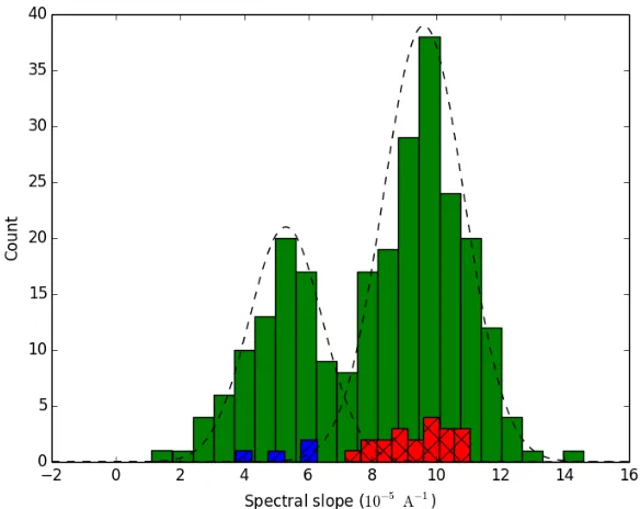
2.1 Distribution of spectral slopes of all 254 Trojans in the Sloan sample with H < 12.3 (solid green), and the distributions of spectral slopes of 24 Trojans classified into the LR and R populations per Emery et al. (2011) and Grav et al. (2012) (blue with diagonal hatching and red with cross hatching, respectively). The best-fit Gaussian distribution functions for the two color populations are shown as black dashed lines. 14 2.2 Plot of the unscaled cumulative magnitude distributions for the main

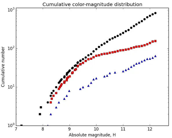
Trojan sample (black circles) and the categorized R and LR color populations (red squares and blue triangles, respectively). These data have not yet been corrected for incompleteness. . . 16 2.3 Plot of the ratio between the cumulative number of objects in the Sloan

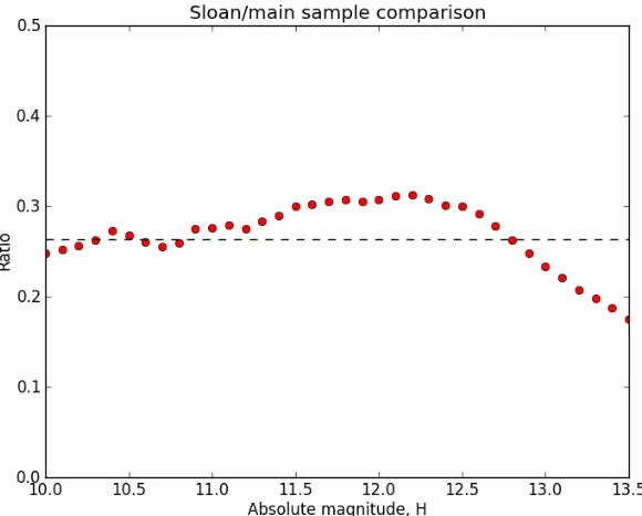
sample and the cumulative number of objects in the main sample for various absolute magnitude bins (red circles). The black dashed line indicates the average valueR∗for bins withH =10.0→ 11.2. . . 18 2.4 Plot depicting the scaled (white squares) and unscaled (black circles)

cumulative magnitude distributions for the total Trojan population, along with the best-fit curve describing the true Trojan cumulative distribution. . . 21 2.5 Plot depicting the scaled (magenta squares) and unscaled (red circles)

cumulative magnitude distributions for R population, along with the best-fit curve describing the true cumulative distribution. . . 22 2.6 Plot depicting the scaled (cyan triangles) and unscaled (blue circles)

cumulative magnitude distributions for LR population, along with the best-fit curve describing the true cumulative distribution. . . 23 2.7 Comparison between the results from the best test run (α1 = 1.11,

α2 = 0.47, H0 = 7.09, Hb = 8.16,c = 6, k = 4.5) and the observed

(10)

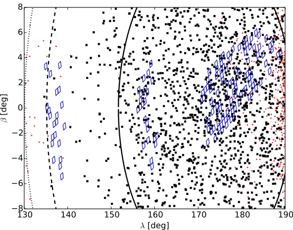
3.1 Locations of the 147 observed Subaru Suprime-Cam fields, projected in geocentric ecliptic longitude-latitude space (blue diamonds). The size of the diamonds corresponds to the total field of view of each image. The positions of numbered Trojans and non-Trojans during the time of our observations with apparent sky motions in the range 14 ≤ |v| < 2200/hr are indicated by black squares and red dots, respectively. The solid, dashed, and dotted curves denote respectively the approximate 50%, 10%, and 5% relative density contours in the sky-projected L4 Trojan distribution (Szabó et al. 2007). . . 40 3.2 Distribution of apparent RA and Dec velocities for numbered Trojans

(black squares) and non-Trojans (red dots) with positions in the range 130◦ ≤ λ < 190◦and −8◦ ≤ β < 8◦. The dotted curves denote the

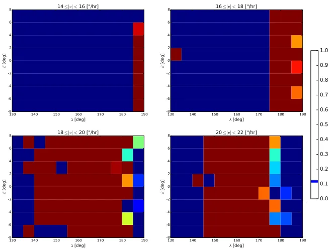
|v| = 1400/hr and |v| = 2200/hr contours, which separate the Trojans from the majority of non-Trojan minor bodies. . . 42 3.3 Map of Trojan fraction γ among numbered minor bodies at various

locations in the space of ecliptic longitude, ecliptic latitude, and apparent sky motion during the time of our observations. Regions in dark red have 0% predicted contamination by non-Trojans, and our operational Trojan data set includes only objects detected in observed fields located within these regions. . . 43 3.4 Seeing of the worst image (highest seeing) in every chip for each set

of four exposures in the 147 observed fields, plotted as a function of the first exposure time. The dotted line indicates the cutoff at 1.200 seeing – objects in fields with higher seeing (red triangles) are not included in the filtered Trojan set. . . 46 3.5 Comparison of the measured standard deviation error in the

differ-ence ofgmagnitudes,σ∆g, binned in 0.5 mag intervals (blue squares)

with the corresponding values from our empirical model combining the measured photometric magnitude errors with a constant contri-bution from asteroid rotation (green squares). The binned medians of the photometric errors only are denoted by black crosses. The agree-ment between the measured and modeled σ∆gvalues shows that the

(11)

3.6 Cumulative absolute magnitude distribution of the filtered Trojan set from our Subaru observations, binned by 0.1 mag (green dots). The best-fit broken power law curve describing the distribution is overplotted (solid black line), with the power law slopes indicated. The dashed line is an extension of theα1= 0.45 slope and is included to make the slope rollover more discernible. . . 50 3.7 Cumulative magnitude distribution of all L4 Trojans contained in the

Minor Planet Center (MPC) catalog brighter than H = 12.3 (white squares; corrected for incompleteness in the range H = 11.3−12.3 following the methodology of Wong et al. 2014) and the cumulative magnitude distribution of the filtered Trojan set from our Subaru observations, approximately scaled to reflect the true overall number and binned by 0.1 mag (green dots). The error bars on the scaled Subaru Trojan magnitude distribution (in green) denote the 95% confidence bounds derived from scaling the Poisson errors on the Subaru survey data. The uncertainties on the corrected MPC catalog Trojan magnitude distribution in the range H = 11.3− 12.3 are much smaller than the points. The best-fit broken power law curves describing the MPC and Subaru data are overplotted (solid black and dashed red lines, respectively), with the power law slopes (in the text: α0

0,α

0

1,α1, andα2) indicated for their corresponding magnitude regions. 51 3.8 Cumulative magnitude distribution of the less-red and red L4 Trojan

populations, as constructed using the methods of Wong et al. (2014) for objects in the Minor Planet Center catalog throughH =12.3 (cyan triangles and red squares, respectively). These distributions have been scaled to correct for catalog and categorization incompleteness; the error bars denote the 95% confidence bounds and are derived from the binomial distribution errors associated with correcting for uncategorized less-red and red Trojans, as well as the uncertainties from the catalog incompleteness correction in the range H = 11.3−

(12)

3.9 Histogram of theg−icolor distribution for Trojans contained in the SDSS-MOC4 catalog brighter thanH =12.3 (green) and fainter Tro-jans detected in our Subaru survey (blue). There is clear bimodality in the distribution of brighter objects in the SDSS-MOC4 catalog, while the distribution of faint Trojan colors does not display a clear bimodality. This is likely due to the large relative uncertainties as-sociated with the measurement of faint Trojan colors due to asteroid rotation. . . 55 3.10 Meang−i colors and corresponding uncertainties for the combined

set of Trojans detected in our Subaru survey and L4 Trojans listed in SDSS-MOC4 (blue squares with error bars). Red dots denote the predicted mean g−i color values computed from extrapolation of the best-fit less-red and red population magnitude distributions, assuming mean less-red and red colors of 0.73 and 0.86, respectively. The mean less-red and redg−icolors are indicated by dashed green lines. The monotonic decrease in mean g −i color indicates an increasing fraction of less-red Trojans with decreasing size. The agreement between the extrapolated values and the measured ones suggests that the best-fit color-magnitude distributions derived from bright catalogued Trojans likely extend throughout the magnitude range studied by our Subaru survey. . . 56 3.11 Comparison between the results from the best test run of our

colli-sional simulation (dotted lines) and the observed L4 Trojan magnitude distributions (solid lines). The initial total magnitude distribution for the best test run is a broken power law with α1 = 0.91, α∗₂ = 0.44,

H0 = 7.22, Hb = 8.46, an initial R-to-LR number ratio k = 5.5 and

(13)

3.12 Comparison of the best-fit cumulative magnitude distribution curve from the survey data (solid line) with the final predicted distribution from two collisional simulation runs: (1) test run assuming bodies with collisional strength given by Equation (3.7) (dashed line) and (2) test run assuming strengthless bodies with collisional strength scaling given by Equation (3.8) (dot-dash line). The better agreement of the latter suggests that Trojans have very low material strength, similar to comets. . . 62 4.1 Histograms of the measured spectral slope values of small KBOs

(top panel), Centaurs (middle panel), and Trojans (bottom panel). The small KBO and Centaur color distributions include only objects fainter than H = 7 and spectral slope uncertainties smaller than the bin size. Cold classical KBOs have been filtered out by omitting all KBOs with inclinations less than 5◦. Color bimodalities are evident in all three minor body populations; they are labeled with their corresponding relative colors: less-red (LR), red (R), and very red (VR). . . 71 4.2 Sublimation lines in the early Solar System, as a function of formation

(14)

4.3 Pictoral representation of the hypothesis presented in this paper and the major predictions thereof. Panel a depicts the initial state of bodies within a primordial planetesimal disk extending from 15 AU to roughly 30 AU at the moment when the nebular gas dispersed and the objects were first exposed to sunlight. Each body was composed of a pristine mix of rocky material and ices; volatile ice sublimation began. Panel b illustrates the development of the primordial R and VR colors: Objects that formed inside of the H2S sublimation line were depleted in H2S after∼100 Myr and formed a dark, reddish irradiation crust (due primarily to retained methanol). Meanwhile, objects that formed farther out beyond the H2S sublimation line retained H2S on their surfaces and thus developed a much redder coloration. The emplacement of Trojans and KBOs during the Nice model dynamical instability is denoted in panel c. We expect that the primordial R and VR objects became R and VR KBOs and Centaurs, respectively, while the Trojans experienced surface color evolution, maintaining the initial color bimodality but resulting in relatively less red colors. Panel d describes the result of collisions in the current Trojan and KBO populations: The surfaces of Trojan collisional fragments of Trojans become depleted in all volatile ice species, thereby becoming LR objects. Although no observational evidence exists at present, we propose that the collisional fragments of small KBOs likely retain H2S on their surfaces, eventually developing into VR objects. . . 79 5.1 Distribution of the 3801 objects in our Hilda dataset, plotted in the

space of semi-major axis (a), eccentricity (e), and inclination (i). Objects belonging to the Hilda and Schubart collisional families are denoted by magenta and yellow dots, respectively; background Hildas are denoted by blue dots. . . 90 5.2 Cumulative absolute magnitude distributions of the total Hilda

(15)

5.3 Top panel: the overall spectral slope distribution of Hildas, as de-rived from SDSS-MOC4 photometry, demonstrating a robust color bimodality that divides the population into less-red and red objects. Bottom panel: the spectral slope distributions for Hilda and Schubart family members, as well as background non-family members. Note that the background color distribution is bimodal, while the individual collisional family color distributions are both unimodal. . . 93 5.4 The cumulative magnitude distributions of the LR and R sub-populations,

where objects (including family members) have been categorized into the sub-populations by spectral slope. The distributions are statis-tically distinct from each other at the 98% confidence level. Both distributions have a characteristically wavy shape that is not consis-tent with a single or double power law curve. . . 95 5.5 Comparison of the Hilda and Trojan color distributions, with family

members removed. For Hildas, all objects brighter than H = 14 are shown, while for Trojans, all objects brighter than H = 12.3 are shown; these are the established completeness limits of the cor-responding analyses (see Wong et al. 2014 for the discussion of Trojans). Both distributions show a clear bifurcation in color, cor-responding to the LR and R sub-populations present in both popula-tions, with comparable mean colors. The R-to-LR number ratio in both Hilda and Trojan background populations are also similar. . . . 96 5.6 Comparison of the total cumulative magnitude distributions of Hildas

(black dots) and Trojans (blue squares). The Trojan distribution has been corrected for incompleteness, following the methods of Wong et al. (2014). The Hilda magnitude distribution is notably shallower throughout the entire magnitude range of the data. . . 99 6.1 Locations of the 52 Subaru Hyper Suprime-Cam fields observed as

(16)

6.2 Distribution of heliocentric distance for the 372 asteroids detected in our survey. Objects with heliocentric distances greater than 30 AU are classified as KBOs, while the closer-in objects are Centaurs. The typical uncertainty of our heliocentric distance estimates is 3.5 AU. . 110 6.3 Histogram of g − i colors for hot KBOs detected in our survey:

the unfilled graph shows the distribution of all 136 objects in the dataset, while the filled graph shows the distribution of only the 118 objects with color uncertainties σg−i ≤ 0.15. A robust bimodality

is evident in both distributions, dividing the objects into two sub-populations — red (R) and very red (VR). The vertical dashed lines indicate the computed mean colors of the R and VR sub-populations —(g−i)_R =0.91 and(g−i)_{V R}= 1.42. . . 113 6.4 Absolute H magnitude distributions of the total survey hot KBO

dataset (black points), as well as the categorized R and VR sub-populations (magenta squares and red triangles, respectively). The error bar in the lower right represents the typical magnitude uncer-tainty: 0.2 mag. The two color-magnitude distributions have very similar shapes throughout the entire magnitude range. The dashed green line indicates the best-fit power law distribution to the total magnitude distribution through Hmax = 7.5, which has a power law slope ofα= 1.45. . . 115 6.5 Top panel: spectral slope distribution of 200 hot KBOs,

(17)

6.6 Color-magnitude plot for hot KBOs and Centaurs combining data tab-ulated in Peixinho et al. (2015) (dots) and the results of our Subaru survey (squares). Only spectral slope measurements with uncertain-ties less than 10×10−5 Å−1 are included; error bars on data points are omitted for the sake of clarity, with the size of the maximum uncertainty indicated by the example error bar in the upper right. Bi-modality in color is discernible among all objects fainter thanH∼ 7. The horizontal dashed line indicates the approximate boundary be-tween R and VR colors. Meanwhile, the larger hot KBOs display a uniform color distribution, with the exception of a small clustering of neutral colored objects in the range H = 2−6 that is dominated by Haumea collisional family members. . . 120 7.1 Average of spectra in the LR and R Hilda sub-populations, normalized

to unity at 2.2 µm. The two spectra are averages of 12 and 14 individual object spectra, respectively. Gray bars mark regions of strong telluric water vapor absorption. The two sub-populations are distinguished primarily by the difference in spectral slope at shorter near-infrared wavelengths (λ < 1.5). The error bars shown here and in subsequent figures are the uncertainties on the individual reflectance values derived from the weighted average of individual object spectra. . . 135 7.2 Comparison of combined visible and near-infrared average spectra of

(18)

7.3 Two-color plot derived from the near-infrared spectra of Hildas (col-ored points) and Trojans (black points). Hildas that are classified as less-red (LR) and red (R) via visible color and/or infrared reflectivity are denoted by blue and red, respectively; unclassifed objects are marked in yellow. The Hilda near-infrared color distribution lacks the robust bimodality evident in the Trojan data. Nevertheless, LR and R Hildas occupy distinct regions in color space, implying sys-tematically different surface properties and allowing us to classify an additional 4 objects into the LR and R sub-populations. . . 139 8.1 Continuum subtracted average laboratory spectra of the experimental

ice samples with or without the inclusion of H2S ice in the near-ultraviolet and blue optical wavelength region. Notably, the no sulfur spectrum shows a relatively narrow absorption feature centered at around 230 nm, which is absent in the spectrum with sulfur. . . 151 8.2 Average normalized reflectance spectra of LR and R Trojans (from

(19)

LIST OF TABLES

Number Page

(20)

C h a p t e r 1

INTRODUCTION

Understanding the formation and evolution of the Solar System is one of the central objectives of modern astronomy. Over the past century, researchers have utilized the burgeoning body of observations to inform increasingly complex theories of planet accretion and migration. The overarching goal of these endeavors is to synthesize a self-consistent narrative describing the initial conditions of the protoplanetary disk, as well as the various physical and chemical processes that govern planet formation and the subsequent evolution of the Solar System to its current state.

The so-called classical paradigm of solar system formation – the solar nebular disk model – was developed throughout the second half of the 20th century, although the hypothesis of a nebular origin for the protoplanetary disk can be traced back to the 18th century. In short, the solar nebular disk model outlines the initial formation of the protoplanetary disk from the gravitational collapse of a portion of a much larger molecular cloud, perhaps triggered by nearby supernovae in a dense star-forming region (see, for example, Montmerle et al. 2006 and references therein). Subsequent coagulation of dust grains into sub-kilometer sized clumps, followed by pairwise collision-driven hierarchical growth into larger gravitationally-bound planetesimals of tens of kilometers in size, resulted in the formation of planetary-mass embryos throughout the protoplanetary disk. In the inner disk, temperatures were too high to allow for volatile molecules like water and methane to condense, limiting the possible growth of these embryos. Meanwhile, beyond the frost line, the abundance of solid-phase volatile material enabled the rapid formation of much larger embryos, which eventually attained sufficient mass to capture the hydrogen and helium from the surrounding disk into a gaseous envelope and become the giant planets.

(21)

new observations have called into question the idea of a quiescent evolution of the Solar System following the era of planet formation.

Uranus and Neptune currently inhabit a region where the reduced density of the protoplanetary disk and the longer orbital times would have made their formation via hierarchical accretion highly implausible, suggesting that they may have formed closer in to the Sun, nearer to the present-day orbits of Jupiter and Saturn, before migrating outward. The higher-than-expected eccentricities and inclinations of the outer planets likewise point toward a period of planetary migration that transpired sometime after the dispersal of the protoplanetary disk, which would have otherwise damped the eccentricities and inclinations to near zero. The discovery and char-acterization of the irregular satellites of the gas giants, whose orbital and surface properties preclude an in situ formation, as well as the dynamically-excited, yet relatively low-mass Kuiper Belt, further add to the growing list of observations that indicate that significant alterations in solar system architecture likely occurred after the end of planet formation.

In the past few decades, the rapid maturation of the field of exoplanet studies has uncovered a rich diversity of exoplanetary system architectures, many of which bear little resemblance to our Solar System. It has become evident that planetary migration might not only be the key to resolving many of the mysteries of the Solar System, but may also be an important and ubiquitous process that figures prominently in the general evolution of planetary systems throughout the galaxy.

(22)

between the planetesimal and the larger planet, with the result being a gradual outward migration of all the gas giants, with the exception of Jupiter, which moved slightly inward.

It is hypothesized that an eventual mean motion resonance crossing between Jupiter and Saturn set off a period of major dynamical restructuring throughout the middle and outer Solar System. The resonance crossing shifted Saturn outward, which subsequently led to mutual gravitational encounters between Saturn and the ice gi-ants. Afterwards, the arrangement of the giant planets altered dramatically as the ice giants were excited onto eccentric orbits that plowed into the primordial planetesi-mal disk. The disruption of the planetesiplanetesi-mals removed more than 99% of the total mass within the primordial outer solar system disk, thereby explaining the current absence of a dense trans-Neptunian minor body population. Eventually, dynamical friction between the outer planets and the remaining planetesimals damped down the eccentricities of the ice giants to their present-day values, bringing an end to the period of dynamical instability.

Dynamical instability models of solar system evolution have undergone several modifications and refinements since their inception. Some of the more recent models propose a sudden stepwise resonance crossing of Jupiter and Saturn via interactions with an ice giant, which prevents the excessive excitation of the Main Asteroid Belt due to sweeping secular resonances that would occur in the case of a smooth migration toward the mean motion resonance (e.g., Brasser et al. 2009; Nesvorný et al. 2013). Other iterations of these models strive to more precisely reproduce the dynamical structure of the present-day Kuiper Belt by including additional ice giants that are eventually ejected from the Solar System (e.g., Nesvorný & Morbidelli 2012). Nevertheless, numerical simulations of dynamical instability scenarios invariably show that the majority of the initial planetesimal disk was ejected from the Solar System (e.g., Roig & Nesvorný 2015). Of the remaining bodies, some were scattered outward to become the current Kuiper Belt, while others were scattered inward to be captured as irregular satellites or into resonant orbits by Jupiter. The latter group of objects became the present-day Jupiter Trojans and Hilda asteroids, which occupy the 1:1 and 3:2 mean motion resonances with Jupiter, respectively.

(23)

These three asteroid populations provide windows into the earliest epochs of the So-lar System and contain a wealth of information regarding the chemical composition and dynamical processes within the protoplanetary disk, extending from the giant planet region out to the farthest reaches of the young Solar System. An in-depth comparison of their properties serves as perhaps the only available robust empirical test of dynamical instability models. However, due to their greater distance, these minor body populations have not garnered the same level of detailed observational analysis as the more accessible Main Belt. The recent advent of new models of solar system evolution has thrust these asteroids into the forefront of planetary science, and their importance in furthering our understanding of solar system history has become more widely recognized.

Over the last four-and-a-half years, I have embarked on a systematic study of the observable properties of Trojans, Hildas, and KBOs. The results of my analyses represent a significant leap in our knowledge of these hitherto poorly-understood minor bodies. These studies are fundamentally motivated as part of a concerted effort to verify the predictions of current dynamical instability models of solar system evolution, with the specific objective of evaluating the similarities and differ-ences between the characteristics of the various populations in the context of their hypothesized common origin in the outer Solar System.

(24)

yielded the first detailed compositional model of these primordial planetesimals within the framework of the dynamical instability scenario of solar system evolution, which outlines their formation location, the development of color bimodality, and the alterations that have occurred following emplacement into their current locations throughout the middle and outer Solar System.

This thesis represents the culmination of my graduate study probing the relationships between Trojans, Hildas, and KBOs and overviews all the major results of my research as presented in their peer-reviewed, published forms. The detailed analyses of the color and size distribution of Trojans and Hildas are described in Chapters 2 and 5, respectively. The results of my wide-field photometric surveys of small Trojans and KBOs are presented in Chapters 3 and 6, respectively. Chapter 4 explains the hypothesis for the color bimodality evident in all three minor body populations and outlines the major implications of the model for future experimental and observational study. Chapter 7 summarizes the analysis of near-infrared spectra of Hilda asteroids and compares them to corresponding spectra for Trojans. Finally, in Chapter 8, the full body of research is brought together and evaluated alongside the predictions from dynamical instability models of solar system evolution. I also discuss potential fruitful avenues for future follow-up study.

References

Brasser, R., Morbidelli, A., Gomes, R., Tsiganis, K., & Levison, H. F. (2009). “Con-structing the secular architecture of the solar system II: the terrestrial planets”. A&A, 507, 1053.

Gomes, R., Levison, H. F., Tsiganis, K., & Morbidelli, A. (2006). “Origin of the cataclysmic Late Heavy Bombardment period of the terrestrial planets”. A&A, 455, 725.

Levison, H. F., Bottke, W., Gounelle, M., et al. (2008a). “Chaotic capture of plan-etesimals into regular regions of the Solar System. II. Embedding comets in the asteroid belt”. In:AAS/Division of Dynamical Astronomy Meeting 39 #12.05.

Levison, H. F., Morbidelli, A., Van Laerhoven, C., & Gomes, R. (2008b). “Origin of the structure of the Kuiper belt during a dynamical instability in the orbits of Uranus and Neptune”.Icarus, 196, 258.

(25)

Morbidelli, A., Levison, H. F., Tsiganis, K., & Gomes, R. (2005). “Chaotic capture of Jupiter’s Trojan asteroids in the early Solar System”.Nature, 435, 462.

Nesvorný, D. & Morbidelli, A. (2012). “Statistical study of the early Solar System’s instability with four, five, and six giant planets”.AJ, 144, 117.

Nesvorný, D., Vokrouhlický, D., & Morbidelli, A. (2013). “Capture of Trojans by jumping Jupiter”.ApJ, 768, 45.

Roig, F. & Nesvorný, D. (2015). “The evolution of asteroids in the jumping-Jupiter migration model”.AJ, 150, 186.

(26)

C h a p t e r 2

THE DIFFERING MAGNITUDE DISTRIBUTIONS OF THE TWO

JUPITER TROJAN COLOR POPULATIONS

Wong, I., Brown, M. E., & Emery, J. P. (2014). “The differing magnitude distribu-tions of the two Jupiter Trojan color populadistribu-tions”.AJ, 148, 112.

ABSTRACT

The Jupiter Trojans are a significant population of minor bodies in the middle

Solar System that have garnered substantial interest in recent years. Several

spectroscopic studies of these objects have revealed notable bimodalities with

respect to near-infrared spectra, infrared albedo, and color, which suggest the

existence of two distinct groups among the Trojan population. In this paper, we

analyze the magnitude distributions of these two groups, which we refer to as

the red and less-red color populations. By compiling spectral and photometric

data from several previous works, we show that the observed bimodalities are

self-consistent and categorize 221 of the 842 Trojans with absolute magnitudes

in the range H < 12.3 into the two color populations. We demonstrate that

the magnitude distributions of the two color populations are distinct to a high

confidence level (>95%) and fit them individually to a broken power law, with

special attention given to evaluating and correcting for incompleteness in the

Trojan catalog as well as incompleteness in our categorization of objects. A

comparison of the best-fit curves shows that the faint-end power-law slopes are

markedly different for the two color populations, which indicates that the red

and less-red Trojans likely formed in different locations. We propose a few

hypotheses for the origin and evolution of the Trojan population based on the

analyzed data.

2.1 Introduction

(27)

than a century ago, thousands of Trojans have been confirmed, and the current catalog contains over 6000 objects ranging in size from 624 Hektor, with a diameter of roughly 200 km, to subkilometer-sized objects. Estimates of the total number of Trojans larger than 1 km in diameter range from ∼1.0 × 105 (Nakamura & Yoshida 2008) to ∼2.5× 105 (Szabó et al. 2007), corresponding to a bulk mass of approximately 10−4 Earth masses. These values are comparable with those calculated for main belt asteroids of similar size, making the Trojans a significant population of minor bodies located in the middle Solar System. The orbits of Trojans librate around the stable Lagrangian points with periods on the order of a hundred years and are stable over the age of the Solar System, although long-timescale dynamical interactions with the other outer planets decrease the regions of stability and lead to a gradual diffusion of objects from the Trojan swarms (Levison et al. 1997). Escaped Trojans may serve as an important source of short-period comets and Centaurs, a few of which may have Earth-crossing orbits (Marzari et al. 1997).

(28)

The current understanding of the composition of Trojan asteroids remains incom-plete. Visible spectroscopy has shown largely featureless spectra with spectral slopes ranging from neutral to moderately red (e.g., Dotto et al. 2006; Fornasier et al. 2007; Melita et al. 2008). Spectroscopic studies of Trojans have also been carried out in the near-infrared, a region which contains absorption bands of materials prevalent in other minor body populations throughout the Solar System, such as hydrous and anhydrous silicates, organics, and water ice (e.g., Emery & Brown 2003; Dotto et al. 2006; Yang & Jewitt 2007; Emery et al. 2011). These spectra were likewise found to be featureless and did not reveal any incontrovertible absorption signals to within noise levels. As such, models of the composition and surface properties of Trojans remain poorly constrained. However, several authors have noted bimodality in the distribution of various spectral properties: Bimodality in spectral slope has been detected in both the visible (Szabó et al. 2007; Roig et al. 2008; Melita et al. 2008) and the near-infrared (Emery et al. 2011). The infrared albedo of Trojans has also been shown to display bimodal behavior (Grav et al. 2012). These observations indicate that the Trojans may be composed of two separate sub-populations that categorically differ in their spectroscopic properties.

While future spectroscopic study promises to improve our knowledge of Trojan com-position and structure, a study of the size distribution, or as a proxy, the magnitude distribution, may offer significant insight into the nature of the Trojan population. The magnitude distribution preserves information about the primordial environment in which the Trojans were accreted as well as the processes that have shaped the population since its formation, and can be used to test models of the origin and evolution of the Trojans. In particular, an analysis of the distribution of the attested sub-populations may further our understanding of how these sub-populations arose and how they have changed over time. In this paper, we use published photometric and spectroscopic data to categorize Trojans into two sub-populations and compare their individual magnitude distributions. When constructing the data samples, we evaluate and correct for incompleteness to better model the true Trojan population. In addition to fitting the magnitude distributions and examining their behavior, we explore various interpretations of the data.

2.2 Trojan data

(29)

Selection of Trojan data samples

The primary data set contains Trojan asteroids listed by the Minor Planet Center (MPC),1 which maintains a compilation of all currently confirmed Trojans. The resulting data set, referred to in the following as the main sample, contains 6037 Trojans. Of these, 3985 are from the L4 swarm and 2052 are from the L5 swarm, corresponding to a leading-to-trailing number ratio of 1.95. This significant number asymmetry between the two swarms has been widely noted in the literature and appears to be a real effect that is not attributable to any major selection bias from Trojan surveys, at least in the bright end of the asteroid catalog (Szabó et al. 2007). The brightest object in the main sample has an absolute magnitude of 7.2, while the faintest object has an absolute magnitude of 18.4. The vast majority of Trojans in the main sample (4856 objects) haveH ≥ 12.5, with most of these faint asteroids having been discovered within the last 5 years. In the literature, estimates of the threshold magnitude below which the current total Trojan asteroid catalog is complete lie within the rangeH ∼10.5−12. Therefore, it is only possible to adequately analyze the magnitude distribution of faint Trojans if appropriate scaling techniques are invoked to correct for sample incompleteness. These techniques are discussed in Section 2.3.

Another data set used in this work consists of observations from the fourth release of the Moving Object Catalog of the Sloan Digital Sky Survey (SDSS-MOC4). The SDSS-MOC4 contains photometric measurements of more than 470,000 moving objects from 519 observing runs obtained prior to March 2007. Of these objects, 557 have been identified to be known Trojans listed in the ASTORB file (243 from L4and 314 from L5), and will be referred to in the following as the Sloan sample. This data sample includes measured flux densities in theu, g, r, i, zbands, centered at 3540, 4770, 6230, 7630, and 9130 Å, respectively, and with bandwidths of∼100 Å. As discussed in detail by Szabó et al. (2007), the distribution of the positions of SDSS observing fields through June 2005 in a coordinate system centered on Jupiter indicates that both L4 and L5 Trojan swarms were well-covered (i.e., the positions of the observing fields cover a wide range of orbital eccentricity and relative longitude values consistent with Trojan asteroids). Those authors identified 313 known Trojans in the SDSS-MOC3 (previous release) and determined that the survey detected all known Trojans within the coverage area brighter thanH = 12.3. Observing runs since then have expanded the coverage of the sky to include new

(30)

Trojan swarm regions, yielding 244 additional known Trojans. It is expected that the detection threshold of the Sloan survey (i.e., magnitude to which the SDSS has detected all Trojans within its observing fields) in these newly-covered regions is similar to that determined for the previously-covered regions, and therefore, we may consider our Sloan sample to be a reliable subset of the total Trojan population up to H ∼ 12.3. This means that the detection threshold of the Sloan sample lies at least 1 mag fainter than the completeness limit of the main sample mentioned above. As part of the analysis presented in the next section, we will confirm the detection threshold of the Sloan sample and use it to arrive at a better estimate of the completeness of the main sample.

Categorizing Trojans

Recent observational studies have identified bimodality in the Trojan population with respect to various photometric and spectroscopic quantities. In this work, we used three earlier analyses of Trojans to classify objects into two color populations.

(31)

(64 objects).

Grav et al. (2012) presented thermal model fits for 478 Trojans observed with the Wide-field Infrared Survey Explorer (WISE), which conducted a full-sky survey in four infrared wavelengths: 3.4, 4.6, 12, and 22µm (denoted W1, W2, W3, and W4, respectively). Using the survey data, the W1 albedo was computed for each object, and it was shown that the distribution of the W1 albedos as a function of diameter is discernibly bimodal for the 66 objects with diameters larger than∼60 km, which corresponds to objects brighter thanH ∼ 9.6; for the smaller (fainter) Trojans, the errors in the measured albedos are much larger, and a clear bimodality would not be able to be discerned. Among these 66 large Trojans, 51 have W1 albedo values between 0.11 and 0.18 (Group A), while 15 have W1 albedo values between 0.05 and 0.10 (Group B). Within each group, the albedo values show no dependence on diameter and are tightly clustered, with average separations between adjacent albedo values of 0.001 and 0.004 for Group A and Group B, respectively. Most importantly, when considering the Trojans that are in both the Grav et al. (2012) and the Emery et al. (2011) data sets, one finds that every object in Group A is a member of Group I, and every object in Group B is a member of Group II, with the sole exception of 1404 Ajax, which has high H-K and 0.85-J color indices characteristic of redder Group I objects, but a relatively low W1 albedo value of 0.085. This correspondence between groups categorized with respect to different spectroscopic quantities reinforces the proposal presented by Emery et al. (2011) that the Trojans are composed of two distinct populations with dissimilar spectral properties and likely different compositions. In particular, we conclude that Group I and Group A are both sampled from one of the two Trojan populations; these objects have redder color indices, and we will refer to this population as the red (R) population. Analogously, Group II and Group B are both sampled from the second Trojan population, which will be referred to as the less-red (LR) population, due to the relatively lower near-infrared color indices of its members.

(32)

photometric data from the Sloan survey.

Roig et al. (2008) studied 250 known Trojans from the SDSS-MOC3 and computed spectral slopes from the listed u, g, r, i, z band flux densities. The authors noted that the distribution of spectral slopes is bimodal. We expanded on this study, reproducing the spectral slope calculations and including new Trojans listed in the SDSS-MOC4. Following the procedure used in Roig et al. (2008), we corrected the flux densities using the solar colors provided in Ivezić et al. (2001): cu−r =

(u−r) −1.77,cg−r =(g−r) −0.45,cr−i =(r−i) −0.10, andcr−z = (r−z) −0.14.

The reflectance fluxes (or albedos),F, normalized to 1 in ther band, were defined as: Fu = 10−0.4cu−r, Fg = 10−0.4cg−r, Fi = 100.4cr−i, and Fz = 100.4cr−z. The

relative errors ∆F/F were estimated using the second-order approach in Roig & Gil-Hutton (2006):

∆F/F =0.9210∆c(1+0.4605∆c), (2.1)

where the color errors∆care computed as the root-squared sum of the corresponding magnitude errors, e.g., ∆cu−r =

p

(∆u)2+_(∆_r₎2_{. The error in} _F

r was estimated

using ∆cr−r =

√

2∆r. We discarded all asteroid observations that had a relative error greater than 10% in any of the fluxes besides Fu, which usually has larger

errors due to the effects of instrument noise in and around the u-band. We also considered only asteroids with magnitudes in the range H < 12.3, over which the Sloan survey is expected to have detected all Trojans within its survey area.

The resulting asteroid set contains 254 objects (114 in L4 and 140 in L5), 24 of which were included in the Emery et al. (2011) and/or Grav et al. (2012) analyses and previously categorized by spectrum. For each object, the spectral slope S

was computed from a linear least-squares fit to a straight line passing through the fluxes Fg, Fr, Fi, and Fz, taking into account the individual errors ∆F (Fu was

not used in this computation, as per Roig et al. 2008). If an object had multiple observations, the average of the spectral slopes computed for all observations was used. The histogram of spectral slopes is shown in Figure 2.1. From the plot, the bimodality in the spectral slope distribution is evident.2 By fitting the spectral slope distribution with two Gaussians, we found that one of the two modes is centered at S = 5.3×10−5 Å−1, while the other mode is located at higher spectral slopes (i.e., redder colors), with a peak at S = 9.6× 10−5 Å−1; the best-fit Gaussian distribution functions are plotted in Figure 2.1. This two-peaked distribution shape

2_{In Roig et al. (2008), it was reported that only objects in the L4 swarm showed this bimodality}

(33)

[image:33.612.155.447.91.323.2]

Figure 2.1: Distribution of spectral slopes of all 254 Trojans in the Sloan sample withH < 12.3 (solid green), and the distributions of spectral slopes of 24 Trojans classified into the LR and R populations per Emery et al. (2011) and Grav et al. (2012) (blue with diagonal hatching and red with cross hatching, respectively). The best-fit Gaussian distribution functions for the two color populations are shown as black dashed lines.

is similar to the one presented by Emery et al. (2011) for the H− K color index. In particular, the 24 Trojans in the Sloan sample that have already been categorized into LR and R populations (4 in LR and 20 in R) align with the two modes shown in Figure 2.1. Therefore, we can say that objects with spectral slope values consistent with the left mode belong to the LR population, while objects with spectral slope values consistent with the right mode belong to the R population. There is some overlap between the two modes, which makes it difficult to categorize all of the Trojans observed by the SDSS into populations. Nevertheless, we may expand our categorization by adopting conservative break-off spectral slope values: All Trojans withS ≤ 5.3×10−5Å−1were classified as less-red, while all Trojans with

(34)

The estimated 95% detection flux density thresholds for the u, g, r, i, z bands are 22.0, 22.2, 22.2, 21.3, and 20.5, respectively (Ivezić et al. 2001). The average relative band magnitudes for the 151 Trojans in the color populations that were imaged by the SDSS areu−r = 2.08,g−r = 0.62,i−r = −0.26, z−r = −0.42 for R objects and u−r = 2.01, g−r = 0.52, i−r = −0.18, z−r = −0.26 for LR objects. For an object to be listed on the Moving Object Catalog, it must have detections in at least three bands. The detection threshold in the z- and i-bands are the lowest. For objects with the same r-band magnitude, LR objects are less reflective at longer wavelengths, so for objects with magnitudes near the detection thresholds, there is a bias against LR objects. However, the differences between the relative band magnitudes among the two color populations are not large, and this bias is only expected to affect the objects with absolute magnitudes at the very faint end of our considered range and beyond. Therefore, for our data samples, this effect is minor and is not taken into consideration in our analysis.

We have compared three photometric and spectroscopic studies of Trojans and determined that the bimodal behaviors observed in all these studies are consistent and indicative of the existence of two separate color populations. Of the 842 objects in the main sample withH < 12.3, 478 are in the L4swarm, and 364 are in the L5 swarm, which entails a leading-to-trailing number ratio of 1.31. This ratio is notably smaller than the value of 1.93 obtained for the total Trojan catalog, which suggests that there may be major detection biases favoring L4 Trojans among the faintest objects. After categorizing the objects in the main sample, we found that 64 objects belong to the LR population, and 157 objects belong to the R population, while the remaining 621 objects were not categorized because they have either not been analyzed by any of the three studies discussed above or have spectral slope values between 5.3×10−5Å−1and 9.6×10−5Å−1. In Figure 2.2, the cumulative magnitude distribution N(H), i.e., the total number of asteroids with absolute magnitude less than or equal to H, is plotted for the main sample and the two color populations. The distributions plotted here have not been scaled to correct for incompleteness.

2.3 Analysis

(35)

[image:35.612.151.448.84.323.2]

Figure 2.2: Plot of the unscaled cumulative magnitude distributions for the main Trojan sample (black circles) and the categorized R and LR color populations (red squares and blue triangles, respectively). These data have not yet been corrected for incompleteness.

Population distinctness

Previously, we classified Trojans into LR and R populations based on various spec-troscopic quantities. While the observed bimodalies indicate that the two popu-lations differ categorically with respect to several spectral properties, the current lack of understanding of Trojan surface composition makes it difficult to use these spectral properties in studying the origin and evolution of Trojans. Moreover, the distinction in spectroscopic properties does not preclude the possibility that the Trojans are simply a mixed population of LR and R objects, with a constant number ratio between the two populations at each magnitude. To determine whether the two color populations are distinct, we must compare the shape of their distributions.

(36)

may test for population distinctness of the Trojan color samples by using the current LR and R populations as plotted in Figure 2.2, without the need to scale up both populations to correct for incompleteness.

Already from the unscaled cumulative magnitude distributions plotted in Figure 2.2, one can see that the distributions of the color populations are dissimilar. To analyti-cally examine the distinctness of the LR and R populations, we used the two-sample Kuiper variant of the Kolmogorov-Smirnov test (Kuiper-KS test; Press et al. 2007). This nonparametric statistic quantifies the likelihood that two data samples are drawn from the same underlying distribution. It evaluates the sum of the maximum dis-tances of one distribution above and below the other and returns a test decision value,

p, between 0 and 1, which represents the probability that the two data samples are not drawn from the same underlying distribution. The Kuiper-KS test is sensitive to differences in both the relative location and the shape of the two cumulative dis-tributions. It is particularly appropriate when dealing with distributions that differ primarily in their tails, as is the case with the Trojan color populations.

Running the Kuiper-KS test on the two color populations, we obtained ap-value of 0.973. This high test decision value demonstrates that the two color populations are not sampled from a single underlying distribution to a confidence level of 97.3%. In other words, the LR and R Trojan populations are distinct not only with respect to the spectral properties of their members, but also with respect to their overall size/magnitude distributions.

Sample completeness

When analyzing a population distribution, it is important to determine and properly correct for any incompleteness in the data sample. To ensure that our curve-fitting adequately models the true Trojan magnitude distribution, we used the Sloan sample to estimate the incompleteness of the main sample and color populations.

(37)

[image:37.612.158.448.86.319.2]

Figure 2.3: Plot of the ratio between the cumulative number of objects in the Sloan sample and the cumulative number of objects in the main sample for various absolute magnitude bins (red circles). The black dashed line indicates the average value R∗ for bins withH =10.0→ 11.2.

(38)

Figure 2.3 shows the values of R plotted with absolute magnitude. From the plot, the expected behavior described earlier is evident: for bins with H < 11.3, the value of R is roughly constant at R∗ = 0.264, which is the average of R for bins with H = 10.0 → 11.2. (Bright objects were omitted from the average, since the small bin numbers lead to significant scatter in R.) At fainter magnitudes, R

increases untilH = 12.3, after which it decreases rapidly. From this, we conclude that every Trojan brighter than H = 11.3 is contained in the main sample (that is, the total Trojan catalog), while the Sloan sample is complete up toH = 12.3 (that is, contains an unbiased subsample of Trojans), which confirms the completeness limit estimate given in Szabó et al. (2007). Using the calculated values of R, we can now evaluate the catalog efficiencyηmpcof the main sample, i.e., the ratio of the number of Trojansnmpc currently cataloged by the Minor Planet Center to the true number of Trojansn0, in each bin withH < 12.3. ForH < 11.3, the main sample is complete, so ηmpc = 1. For 11.3 ≤ H < 12.3, we first evaluate the ratio r(H) between the non-cumulative (i.e., differential or bin-only) number of Trojans in the Sloan and main samples for each 0.1-mag bin; the values ofr(H) in this interval are greater than the benchmark value ofr∗ = r¯ = 0.29, where ¯r is the average of

r(H) over the interval H = 10.0 → 11.2. The catalog efficiency value for each bin is given by r(∗)/rH. We subsequently fit a fifth-order polynomial through the

binned catalog efficiency values over the domain 11.3 ≤ H < 12.3 to arrive at a smooth functional formη1(H). The catalog efficiency can be expressed as a single piecewise-defined function:

ηmpc(H)=

      

1, forH < 11.3

η1(H), for 11.3≤ H < 12.3

. (2.2)

(39)

inclination, with objects at larger inclinations tending to be redder; Fornasier et al. (2007) reported a similar correlation in their study of visible spectral slope and interpreted it as a lack of faint objects with low spectral slope. This color-inclination correlation was found to be the same in both swarms. Szabó et al. (2007) identified a bias in their data: the L5subsample of Trojans had a significantly larger fraction of objects with high inclinations than the L4 subsample. In our analysis, such asymmetric coverage would cause the number ratio of R-to-LR L5 Trojans to be unrealistically inflated and skew the overall color distributions.

To determine whether a similar bias is present among the 254 objects in the current Sloan sample, we computed the fraction of objects in the SDSS-MOC4 with large inclinations (i > 20◦) for the leading and trailing swarms independently. It was found that the fraction is similar for the two swarms (0.24 for L4and 0.22 for L5). This means that observing runs since the release of SDSS-MOC3 have captured more high-inclination regions of the L4 swarm, and as a result, the leading and trailing swarms are equally well-sampled in the SDSS-MOC4 data. Therefore, no selection bias with respect to inclination is discernible in the Sloan sample, and we may consider the LR and R color populations defined in Section 2.2 to be a representative subset of the true color composition of the overall Trojan population. In particular, the number ratio of red to less-red Trojans in each bin should be approximately the same as the true ratio at that magnitude. We define a categorization efficiency value for each bin, which is the ratio between the number of already-categorized Trojans in the LR and R populations, nL R(H)+ nR(H), and the total number of detected

Trojans,ndet(H). Over the domain 9.6≤ H < 12.3, where the color classification is incomplete, we followed a similar procedure to that used in deriving the detection efficiency and fitted a polynomial through the categorization efficiency values to obtain a smooth functionη2(H). We can write the overall categorization efficiency function as

ηcat(H)=

      

1, forH < 9.6

η2(H), for 9.6≤ H <12.3

. (2.3)

This categorization efficiency function is the same for both LR and R populations and must be coupled with the detection efficiency functionηdet(H)forH ≥ 11.3.

The total efficiency functions for the main sample and color populations, which take into account catalog and/or categorization incompleteness, are given by

η(H)=

      

ηmpc(H), for the main sample

ηcat(H) ×ηmpc(H), for the LR and R populations

(40)

[image:40.612.152.449.87.322.2]

Figure 2.4: Plot depicting the scaled (white squares) and unscaled (black circles) cumulative magnitude distributions for the total Trojan population, along with the best-fit curve describing the true Trojan cumulative distribution.

We used catalog and categorization efficiency to scale up the data samples so that they approximate the true Trojan population. Similar scaling methods have been employed in the study of the size distribution and taxonomy of main belt asteroids (DeMeo & Carry 2013). We demonstrate our method with the following example: At H = 11.5, there are 43 objects in the main sample, 17 of which are also contained in the Sloan sample. The ratio between the number of objects in the Sloan and main samples isr =17/43≈0.395, which yields a catalog efficiency value of η = r∗/r ≈ 0.73. Thus, the approximate true number of Trojans withH = 11.5 is

n0 = 43/η ∼ 59. The scaled and unscaled cumulative magnitude distributions for the main sample and color populations are shown in Figures 2.4-2.6.

Distribution fits

Previous analyses of the magnitude distributions of Trojans (see, for example, Je-witt et al. 2000) have shown that the differential magnitude distribution, Σ(H) =

dN(M)/dH, is well-described by a broken power law with four parameters:

Σ(α₁, α₂,H0,Hb|H)=

      

10α1(H−H0), _for_H < _H

b

10α2H+(α1−α2)Hb−α1H0, _for_H _≥ _H

b

(41)

[image:41.612.151.448.86.322.2]

Figure 2.5: Plot depicting the scaled (magenta squares) and unscaled (red circles) cumulative magnitude distributions for R population, along with the best-fit curve describing the true cumulative distribution.

where there is a sudden change from a bright-end slopeα1to a shallower faint-end slope α2 at some break magnitude Hb. H0 is the threshold magnitude for which Σ(H0) = 1 and serves to properly normalize the distribution to fit the data. Jewitt

et al. (2000) obtained the slope valuesα1= 1.1 andα2= 0.4 from their study of 257 Trojans, which did not correct for incompleteness in the faint-end distribution. More recent studies of faint Trojans by Szabó et al. (2007) and Yoshida & Nakamura (2005) obtained faint-end slope values of 0.44 and 0.38, respectively.

(42)

[image:42.612.151.448.84.323.2]

Figure 2.6: Plot depicting the scaled (cyan triangles) and unscaled (blue circles) cumulative magnitude distributions for LR population, along with the best-fit curve describing the true cumulative distribution.

efficiency can be easily integrated into the formulation.

The likelihood function used in our fitting takes the form

L(α₁, α₂,H0,Hb|Hi) ∝e−N

Ö

i

Pi, (2.6)

whereHiis the absolute magnitude of each detected Trojan,Nis the total number of

detected objects expected in the magnitude range under consideration, andPiis the

probability of having objecti with magnitudeHi given the underlying distribution

functionΣ. Taking into account detection and categorization incompleteness,N is given by

N =

∫ Hmax

−∞

η(H)Σ(α₁, α₂,H0,Hb|H)dH, (2.7)

whereη(H)is the efficiency function defined in Equation (2.4), and Hmax = 12.3.

(43)

The best-fit distribution functions were obtained by maximizing the likelihood func-tion over the four-dimensional parameter space using an affine-invariant Markov Chain Monte Carlo (MCMC) Ensemble sampler with 100,000 steps (Foreman-Mackey et al. 2013). The optimal parameters and corresponding 1σ errors were computed for each distribution. The magnitude distribution of the main sample (all Trojans with H < 12.3) is best-fit by α1 = 1.11± 0.20, α2 = 0.46± 0.01,

H0 = 7.09+₋0₀._.03₀₂, and Hb = 8.16+₋0₀._.03₀₄. The bright-end slope is consistent with

the value calculated in Jewitt et al. (2000), while the faint-slope is steeper than previously-obtained values, due to our correction for incompleteness in the Trojan catalog past H = 11.3. The L4 and L5 Trojans were independently analyzed for detection completeness and fitted in a similar fashion. The optimal values of the slopes α1 and α2 for the two swarm distributions were found to be indistinguish-able within calculated uncertainties. This agrees with the results of earlier studies (see, for example, Yoshida & Nakamura 2008) and demonstrates that the leading and trailing Trojan swarms have magnitude distributions that are identical in shape, differing only in overall asteroid number.

The magnitude distributions of the color populations were both individually fitted to a broken power law. The optimal parameters for the R population magnitude dis-tribution areα1 =0.97+₋0₀_..₀₄05,α2 =0.38±0.02, H0 =7.24+₋0₀._.05₀₇, andHb =8.70+₋0₀._.08₁₁,

while for the LR population magnitude distribution, they are α1 = 1.25+₋0₀._.09₀₄,

α2 = 0.52₋+0₀_..03₀₁, H0 = 7.77₋+₀0._.04₀₉, and Hb = 8.15+₋0₀._.06₁₀. Figures 2.4-2.6 show the

cumulative magnitude distributions for the main sample and the color populations, along with the best-fit curves that describe the true distributions. In each plot, the lower distribution is the cumulative count for the unscaled data set, and the upper distribution is the approximate true distribution, scaled to correct for catalog and/or categorization incompleteness (as described earlier).

2.4 Discussion

(44)

The most notable feature of the magnitude distributions is the transition from a steep power-law slope to a shallower slope atH ∼8−9. Previous studies of the total Trojan magnitude distribution (e.g., Morbidelli et al. 2005) have suggested that the broken power-law shape separates the population into two groups: Objects with magnitudes brighter than the break magnitude are described by a power-law slope that reflects the primordial accretion processes that created the original Trojan population. On the other hand, objects with magnitudes fainter than the break magnitude form a sub-population that has reached collisional equilibrium and is mostly composed of collisional fragments of larger objects. It was demonstrated in pioneering work by Dohnanyi (1969) that the magnitude distribution of a small body population that evolves solely through self-collisions attains an equilibrium power-law slope of α∗ ∼ 0.5 when collisional equilibrium is achieved, regardless of the initial shape of the distribution. The faint-end slope of the total Trojan magnitude distribution that we obtained by fitting the data is α2 = 0.46±0.01, which is consistent with the canonical collisional equilibrium slope. In relation to the history of the Trojan population, there arises the question of whether the sharp roll-over to a shallower faint-end slope in the currently-observed population is a consequence of collisional evolution after the Trojans were emplaced in their current orbits around Jupiter, or a result of collisional interactions in the primordial trans-Neptunian region prior to emplacement. Several authors have modeled the collisional evolution of Trojans and determined that the observed broken power-law distribution is best reproduced when assuming that a break was present at the time of emplacement (c.f., Marzari et al. 1997; de Elía & Brunini 2007). Furthermore, these studies have shown that the intrinsic collision probabilities characteristic of the Trojan swarms are insufficiently high to have brought about any significant collisional evolution among objects with magnitudes brighter than the break. Thus, the currently-observed bright-end distribution reflects the shape of the primordial size distribution of large Trojans at the time of emplacement.

(45)

color distributions yielded intermediatep-values, which are inconclusive as a metric for population distinctness.) A hypothesis that posits a scenario in which the two color populations arose from different regions in the primordial trans-Neptunian disk would be able to explain the different bright-end slopes, which are determined primarily by the accretion environment. However, in light of the interpretation that the faint-end portion of the broken power-law distributions is a result of col-lisional evolution, the significant difference between the faint-end slopes poses a challenge. One possible explanation would be that just as different accretion envi-ronments can lead to different bright-end slopes, non-uniform collisional dynamics in the primordial trans-Neptunian disk could have resulted in the color populations experiencing different early collisional histories owing to their different formation regions. Various areas of the primordial disk may have been characterized by a wide range of impact velocities and intrinsic collision probabilities. In such a model, the currently-observed discrepancy between the faint-end slopes would be a relic of the pre-emplacement collisional evolution of the two color populations. Indeed, very little is known about the nature of the early Solar System, so one could not exclude this possibility.

That said, the fact that the overall Trojan population is characterized by a faint-end slope so close to the canonical collisional equilibrium slope suggests that perhaps there is another explanation in which the two color populations experienced a similar collisional evolution within the primordial trans-Neptunian disk and were emplaced with similar faint-end slopes. In this case, the different faint-slopes would be explained by positing a mechanism that converts R objects to LR objects, hence flattening the faint-end slope of the R population, while simultaneously steepening the faint-end slope of the LR population.

(46)

R objects to LR ones, one would not expect any R objects to remain. In Melita et al. (2009), an additional mechanism is proposed whereby minor cratering events disrupt the spectrally flattened irradiation crust and excavate underlying material, which the authors of that work posit as being red in color, consistent with that of typical surfaces rich in complex organic materials. The added contribution of cratering leads to irradiated LR objects becoming R objects once again through resurfacing, thereby preventing all the R objects from turning into LR objects. However, the characteristic collisional timescale and, correspondingly, the timescale of resurfacing decrease with decreasing asteroid size, while the rate of irradiation is the same for all objects, as mentioned earlier. Therefore, the resurfacing of Trojans through cratering becomes more effective at returning irradiated LR objects to R objects when one goes to smaller sizes. This would lead to a relative excess of R objects at faint magnitudes, which is the opposite of what is evident in the observed color distributions.

In this work, we suggest an alternative explanation for the discrepancy in faint-end slopes and examine the possibility that the fragments resulting from a catastrophic shattering impact on a red object are less-red. In other words, we hypothesize that R and LR Trojans have more or less identical interiors, differing only in the spectroscopic properties of their outer surfaces, and that the destruction of red objects is the primary mechanism by which red objects become less-red, thereby resulting in a relative depletion of red Trojans in the range of sizes for which shattering collisions have been significant. To assess the viability of this conversion hypothesis, we ran a series of simple numerical simulations that model the collisional evolution of the Trojan population since emplacement. The mechanics of our algorithm are similar to those used in previous studies of Trojan collisions (c.f., Marzari et al. 1997). Earlier works have shown that the overall Trojan-Trojan collisional frequency among large objects withH > 9 is very low ( 1 per Gyr). This means that most of the collisional activity is concentrated in the faint-end of the magnitude range, and that the magnitude distribution of bright objects is expected to remain almost unchanged over the age of the Solar System. Therefore, we only considered initial magnitude distributions that are broken power-laws of the form described in Equation (2.5) with a bright-end distribution identical to that of the currently-observed population (α1 = 1.11, H0 = 7.09, and Hb = 8.16). For the initial

faint-end slope, we considered values ranging from 0.45 to 0.55, in increments of 0.01. Objects in the initial population with absolute magnitudes in the range

(47)

formula D = 1329× 10−H/5/√pv, where we have assumed a uniform geometric