An improved dissipative particle dynamics scheme

An improved dissipative particle dynamics scheme

N. Mai-Duy

_{, N. Phan-Thien}

_{and T. Tran-Cong}

_{Computational Engineering and Science Research Centre,}

School of Mechanical and Electrical Engineering,

University of Southern Queensland, Toowoomba, QLD 4350, Australia

_{Department of Mechanical Engineering, Faculty of Engineering,}

National University of Singapore, 9 Engineering Drive 1, 117575, Singapore

Submitted to Applied Mathematical Modelling, Oct/2016;

revised Jan/2017

ABSTRACT: Dissipative particle dynamics (DPD) and smoothed dissipative particle dy-namics (sDPD) have become most popular numerical techniques for simulating mesoscopic flow phenomena in fluid systems. Several DPD/sDPD simulations in the literature indi-cate thatthe model fluids should be designed with their dynamic response, measured by the Schmidt number, in a relevant range in order to reach a good agreement with the experimen-tal results. In this paper, we propose a new dissipative weighting function (or a new kernel) for the DPD (or the sDPD) formulation, which allows both the viscosity and the Schmidt number to be independently specified as input parameters. We also show that some existing dissipative functions/kernels are special cases of the proposed one, and the imposed viscosity of the present DPD/sDPD system has a lower and upper limit. Numerical verification of the proposed function/kernel is conducted in viscometric flows.

Keywords: Dissipative particle dynamics, kinetic theory, weighting functions, kernel func-tions, Schmidt number, mesoscale fluid systems.

1

Introduction

Dissipative particle dynamics (DPD) was introduced in 1992 by Hoogerbrugge and Koelman [1] as a coarse graining of molecular dynamics, intended for modelling complex fluids on a mesoscopic length scale. In DPD, the fluid, and everything in it, is represented by a set of particles (called DPD particles) that are free to move in space, each is supposed to represent a group of (molecular) particles. The motions of these DPD particles are governed by Newton’s second law, where the forces acting on each particle consist of a conservative, a dissipative and a random forces. These forces drop off to zero outside a cut-off radius (which may be different for different types of forces). The conservative force is employed to provide a means to control the compressibility of themodel fluid independently of the number densityn, the cut-off radius rc and the equilibrium temperature kBT (mean specific kinetic energy) [2].

∗_{Corresponding author E-mail: nam.mai-duy@usq.edu.au, Telephone 46312748, Fax}

The dissipative force models viscous actions or hydrodynamic behaviour, which slows down the particles and thus to extract the system energy. The random force injects the kinetic energy to the DPD system to compensate for the lost energy due to dissipation. Later on, the DPD system is enforced to satisfy a thermal equilibrium according to a fluctuation-dissipation theorem (sometimes called detailed balance), resulting in some constraints on the dissipative and random forces [3]. All the DPD forces are pairwise, and are centre to centre. It should be pointed out that the DPD system conserves mass and momentum, both linear and angular, whilst maintains a constant temperature (specific kinetic energy) [4]. The DPD equations are stochastic equations that can be re-cast into a differential form by treating the random forces as a Wiener process. The numerical results over a large number of time steps are then averaged in small fixed collection bins to produce local density and local momentum. One can compute the stress tensor by means of Irving-Kirkwood formulation [5], which arises also from the conservation of linear momentum. Furthermore, the method possesses a free-scale property: a DPD system can be scaled so that one deals with a smaller number of particles; different levels of coarse graining with an appropriate scaling lead to the same calculated results [6]. It is noted that the link between the DPD and physical units is still not clear and further studies are needed. DPD can be understood as a bottom-up approach for handling complex fluids on mesoscopic length scale; the complex nature of the fluid is prescribed by the interaction between a subset of DPD particles (for example, chains as representative of polymers in a solution), e.g., [7,8,9].

On the other hand, the smoothed DPD method (sDPD) is a top-down approach for dealing with mesoscopic problems, derived directly from the Navier-Stokes equation with the inclu-sion of thermal fluctuation, where the random force is introduced in a way that satisfies a fluctuation-dissipation theorem [10]. Any non-Newtonian character of the fluid is explicitly specified in the constitutive equation, which is included in the Navier-Stokes equation. It can be seen that the formulations of DPD and sDPD have similar structures as they all involve conservative, dissipative and random forces. However, sDPD allows the viscosity (in fact, the whole rheology of the fluid via its constitutive equation) to be specified and the equation of state (pressure-density) as inputs of the simulation.

DPD and sDPD have been applied to various fluid dynamics problems; however, a complex structure fluid is not always modelled in the same way by the two versions. For example, in simulating particulate suspensions with DPD, a rigid particle can be represented effectively with only one DPD particle (the single particle model) [11], or by a few DPD particles (the spring model) [12,13], improving efficiency of the DPD simulation. To date, with sDPD, suspended particles have been modelled by the frozen particles [14] and thus a very much larger number of particles are required for a given volume fraction.

The dynamic response of a fluid can be measured by its Schmidt number, defined as the ratio of the the speed of momentum transfer (viscosity) to that of particles’ diffusion (diffusivity)

Sc =

η

ρD, (1)

where ρ is the fluid density, η is its viscosity, and D, its diffusivity. For sDPD, in principle, Sc can be arbitrarily large. However, simulations at large values of Sc using the standard

predictor-corrector and velocity-Verlet schemes face a serious time-step limitation. Increasing the time-step size to a realistic value requires a splitting scheme [15]. For DPD, with the “standard” values of the input parameters, it has been shown thatSc isO(1), which is much

lower than that of a typical water-like liquid (e.g., for water,Sc ∼400) [9]. As a result, special

that the Schmidt number of the solvent strongly affects nonequilibrium polymeric quantities [17]. Several studies [17,15] indicated that the model fluidshould be designed with Sc in the

relevant range in order to reach a good agreement with the experimental results. One can improveSc by increasing the strength of the dissipative force, which requires a smaller time

step to maintain temperature control, or simply modifying the standard weighting function for the dissipative force [18]. Analytic expressions for the self-diffusion coefficient have been derived from the kinetic theory for DPD [9,19,2] and from the equation of motion of a single particle for sDPD [20], where the conservative force is neglected in both cases. In both DPD and sDPD, the Schmidt number is a result of the choice of the parameters adopted, it has never been considered before as an input parameter.

In this study, we present some kinetic theory analysis for sDPD, introduce a new dissipative weighting function (or a new kernel) into the DPD (or the sDPD) equations which allows both the viscosity and the Schmidt number ofthe model fluidsto be controlled, and compare the numerical performance in simulating viscometric flows between the proposed DPD (i.e., new dissipative weighting function, repulsion force derived from a soft potential form) and the proposed sDPD (new kernel, repulsion force derived from the discretisation of the pressure gradient term in the Navier-Stokes equation).

2

sDPD and DPD formulations

We briefly recall the isothermal Navier-Stokes equation for a compressible Newtonian fluid of density ρ, dynamic viscosity η0 and volumetric viscosity ζ

dρ

dt =−ρ∇.v, (2)

ρdv

dt =−∇P +η0∇

2

v+ζ+ η0 3

∇∇.v, (3)

wheret is the time, vthe flow velocity and P the pressure.

Smoothed particle hydrodynamics (SPH) interpolations of some of the gradient terms that arise in the Navier-Stokes equation result in [10]

(_∇P)_i di

=₋X

j

Pi

d2

i

+Pj d2

j

Fijrij, (4)

1 di ∇

2 v

i =−2

X

j

Fij

didj

vij, (5)

1 di

(_∇∇.v)_i =₋X

j

Fij

didj

[(_D+ 2)eijeij.vij −vij], (6)

where _D is the number of dimensions, di(= 1/Vi) is the number density of particle i (Vi

is the volume of particle i), eij = rij/rij a unit vector from particle j to particle i (r the

position vector, rij = ri −rj, rij = |rij|), vij = vi −vj the relative velocity vector, and

Fij = −W′(rij, h)/rij with h being the smoothing length of the kernel W which has two

properties: (i) [W]R= 1 and (ii) in the limit h→0,W(r) tends to the Dirac function δ(r).

Here we have employed the notation

[W]R=

Z

Popular kernels in SPH include Lucy and quintic spline functions which are considered in this work.

If incompressibility of the fluid is invoked in the SPH discretisation, i.e., (_∇∇.v)_i = 0, equation (6) leads to [21]

vij = (D+ 2)eijeij.vij. (8)

This gives rise to a SPH approximation of the incompressible isothermal Newtonian N-S equations as

mdvi dt = X j Pi d2 i

+Pj d2

j

rijFijeij −2η0

X

j

Fij

didj

vij, (9)

Pi =P0

" ρi ρ0 7 −1 #

, ρi =mdi, (10)

whereP0 is chosen in a way which results in a large speed of sound that can keep a relative

density fluctuation small [22]. In this study, the relative density fluctuation is chosen less than 1% level, and consequently we choose P0 =c2_sρ0/7 (cs is the speed of sound and ρ0 the

equilibrium (reference) density).

Substitution of (8), from the incompressibility constraint, into (9) yields

mdvi dt = X j Pi d2 i

+ Pj d2

j

rijFijeij −2(D+ 2)η0

X

j

Fij

didj

eijeij.vij. (11)

On a mesoscopic length scale, a fluctuation term is introduced into equation (11) (i.e., a smoothed DPD version) resulting in [10]

mdvi dt = X j Pi d2 i

+Pj d2

j

rijFijeij −2(D+ 2)η0

X

j

Fij

didj

eijeij.vij+

s

2kBT2(D+ 2)η0

X

j

Fij

didj

θijeij, (12)

wherekBT is the equilibrium temperature and θij is a Gaussian white noise.

Returning to the DPD method, the fluid is replaced by a system of DPD particles undergoing their Newton’s second law motion:

mdvi dt =

X

j

(Fij,C +Fij,D+Fij,R), (13)

where m and vi represent the mass and velocity vector of a particlei, and the three forces

on the right hand side represent the conservative force (subscript C), the dissipative force (subscript D) and the random force (subscript R):

Fij,C =aijwCeij, (14)

Fij,D =−γwD(eij·vij)eij, (15)

Fij,R =σwRθijeij, σ=

p

2γkBT , (16)

where aij, γ and σ are constants reflecting the strengths of these forces, wC, wD and wR

that wD(r) and wR(r) are dimensionless functions, γ has the unit of [F T /L] and σ has the

unit of [F√T] ([F], [T] and [L] are the unit of force, time and length, respectively). For

wC, there are several formes proposed, including purely repulsive, attractive-repulsive and

multibody. In the present work, only the original (purely repulsive) form, which has been widely regarded as standard form, is considered. Hereafter, a DPD fluid is referred to as the model fluid corresponding to the purely repulsive form of the conservative force.

Drawing a comparison between (12) and (13), one may identify the different sDPD to DPD forces

aijwC(rij) =

Pi

d2

i

+Pj d2

j

rijFij, (17)

γwD(rij) = 2(D+ 2)η0

Fij

didj

, (18)

σwR(rij) =

s

2kBT2(D+ 2)η0

Fij

didj

, (19)

or

aijwC(rij) =

Pi

d2

i

+Pj d2

j

rijFij, (20)

γ = 2(_D+ 2)rcη0, wD(rij) =

Fij

rcdidj

, (21)

σ =p2kBT2(D+ 2)rcη0, wR(rij) =

s

Fij

rcdidj

. (22)

In both cases, DPD and sDPD, the random force is introduced in a way that satisfies a fluctuation-dissipation theorem.

3

Kinetic theory analysis

The sDDP equation (12) is rewritten in the form of standard DPD ((20)-(22)) and one can thus apply the kinetic theory results in DPD in its analysis [19,2].

In the absence of the conservative force (FC(r) = 0), using the kinetic theory, the expressions

for the viscosity and diffusivity have been derived as [19,2]

η = 3mkBT 2γ[wD]R

+γn

2

[R2

wD]R

30 , (23)

D= 3kBT nγ[wD]R

, (24)

where n is the number density, [wD]R = R dRwD(R) and [R2wD]R = R dRR2wD(R). In

(23), there are two contributions to the viscosity η, a kinetic part (η_K) due to the mo-tion of the individual particles (first term on RHS, called the “gas” contribumo-tion) and a dissipative part (η_D) by the energy dissipation between particles (second term, called the “liquid” contribution). It is noted that, unlike the standard DPD, there are some con-straints onwD(rij) =Fij/(rcdidj) =−(1/(rcdidjrij))(dW/drij) in sDPD (e.g., [W]R= 1 and

In the case of Lucy function, function F(r) takes the form

F(r) =₋1 r dW dr = 315 4πr5 c

1₋ r rc

2

, (25)

where the cut-off radius of the dissipative force (rc) is taken as the smoothing length of

the kernel h. Here, we assume that DPD particles have constant number density (i.e., di =dj =n). For 3D space, we have γ = 2(D+ 2)rcη0 = 10rcη0 and

wD(r) =

F(r) n2_r

c

= 315 4πn2_r6

c

1₋ r rc

2

. (26)

Some simple integrations can be carried out to yield

[wD]R=

Z

dRwD(R) =

315 4πn2_r6

c 4πr3 c 1 30 = 21 2 1 n2_r3

c

, (27)

[R2

wD(R)] =

Z

dRR2

wD(R) =

315 4πn2_r6

c

4πr5

c

1 105 = 3

1 n2_r

c

. (28)

The viscosity (23) reduces to

η=η_K +η_D = 1 70

mkBT n2rc2

η0

+η0. (29)

The possibility of using (29) as a mean to specify an arbitrary viscosity is noted. Expression (29) can be rearranged in the quadratic equation form for the specified input viscosity η0

η02−ηη0+B = 0, B =

1

70mkBT n

2

rc2. (30)

For this to have a physical solution, we require

η2

≥4B = 4

70mkBT n

2

r2

c. (31)

For example, if m = 1, kBT = 1 and n = 4, then η ≥ 0.9562 for rc = 1 and η ≥2.3905 for

rc = 2.5. Suppose that this requirement is met, then the input viscosity can either be

η0 =

1 2η+

1 2

p

η2

−4B or η0 =

1 2η−

1 2

p

η2

−4B. (32)

Since the first solution in (32) is the dissipative part ofηand the second one the kinetic part of η, only the first solution needs be considered if the viscosity for liquid is desired.

The self-diffusion coefficient (24) reduces to

D= 2ηK mn =

1 35

kBT nr2c

η0

. (33)

Consequently, the Schmidt number is

Sc =

η ρD =

35η0η

mkBT n2r2c

. (34)

Substitution of (33) into (34) yields Sc = η/2ηK. At low Schmidt numbers, the kinetic

part of the viscosity thus becomes noticeable. For such Sc values (some gas regime flow),

Consider a generic tagged particle in a sea of other particles undergoing a diffusion process. According to the Stokes-Einstein relation, the size of a tagged particle (exclusion zone) can be estimated as

aef f =

kBT

6πDη. (35)

Substitution of (33) into (35) yields

aef f =

35η0

6πnr2

cη

. (36)

In the case of quintic spline function, using the same derivation procedure, expressions for the viscosity, self-diffusion coefficient, Schmidt number, and the size of a tagged particle are respectively given by

η = 1 120

mkBT n2r2c

η0

+η0, (37)

D = 1 60

kBT nrc2

η0

, (38)

Sc =

60η0η

mkBT n2r2c

, (39)

aef f =

10η0

6πnr2

cη

. (40)

4

Proposed dissipative weighting function/kernel

We propose a kernel that allows one to control both the viscosity and the Schmidt number of the sDPD fluid. The former is achieved by designing the proposed kernel to satisfy the properties of function W in SPH. The latter is achieved by introducing a free parameter, namely s, into the kernel. In other words, from a DPD perspective, there will be 2 free parameters (γ and s) in the dissipative force form and they are used to match the two dynamic thermo-properties, namely η and Sc, of a given fluid. Details are as follows.

4.1

Three dimensional space

To achieve the goals just mentioned, a kernel should be designed (i) to satisfy the properties of function W in SPH; and (ii) to result in function F(r) in the form of (1₋r/rc)s. The

kernel can be verified to be

W(r, rc) =

(s+ 3)(s+ 4)(s+ 5) 32πr3

c

1₋ r rc

s+1

1 + (1 +s)r rc

, s >0, (41)

where s is a free parameter. It has the same properties as SPH kernels (i.e., [W]R = 1 and

limrc→0W(r, rc) =δ(r)). It is noted that when s = 2, the proposed kernel reduces to Lucy

function. The corresponding function F(r) is

F(r) =₋1 r

∂W ∂r =

(s+ 1)(s+ 2)(s+ 3)(s+ 4)(s+ 5) 32πr5

c

1₋ r rc

s

From (42), the weighting function for the dissipative force is derived

wD(r) =

F(r) n2_r

c

= (s+ 1)(s+ 2)(s+ 3)(s+ 4)(s+ 5) 32πn2_r6

c

1₋ r rc

s

. (43)

When s= 1/2, the proposed weighting function reduces to the one reported in [18] which is widely employed in DPD. It can be shown that

[wD]R =

(s+ 4)(s+ 5) 4n2_r3

c

, [R2

wD]R =

3 n2_r

c

. (44)

Using the kinetic theory, the dynamic thermo-properties of the sDPD fluid are estimated as

η=η_K+η_D = 3mkBT 2γ[wD]R

+γn

2

[R2

wD]R

30 =

3 5

mkBT n2r2c

η0(s+ 4)(s+ 5)

+η0, (45)

D= 2ηK mn =

6 5

kBT nrc2

η0(s+ 4)(s+ 5)

, (46)

Sc =

η mnD =

5 6

ηη0(s+ 4)(s+ 5)

mkBT n2r2c

, (47)

aef f =

kBT

6πDη = 5 36

η0(s+ 4)(s+ 5)

πnr2

cη

. (48)

Some conditions on (45)-(47) are required to ensure that the equations have a physical solution. For given values ofm, kBT, n and rc, the minimum value of the viscosity η can be

estimated by considering (45) as an equation for η0. Multiplying both sides of (45) with η0

yields

η2

0 −ηη0+B = 0, B =

3 5

mkBT n2r2c

(s+ 4)(s+ 5), (49) leading to

η_≥√4B =

s

12 5

mkBT n2rc2

(s+ 4)(s+ 5). (50)

For liquid regime (η_{K ≪}η_D),

η_≃η0 ≥

s

12 5

mkBT n2rc2

(s+ 4)(s+ 5). (51)

As mentioned earlier, the free parametersis introduced to makeSc become an input

param-eter to the DPD equation. To achieve this, we consider (47) as an equation for the variable s

s2

+ 9s+ 20₋C = 0, C= 6 5

ScmkBT n2r2c

ηη0 ≃

6 5

ScmkBT n2rc2

η2 0

. (52)

This equation always has two solutions. Since s >0, we choose the following solution

s= −9 +

√

1 + 4C

2 . (53)

If the Schmidt number is given, then the value of s can be estimated from (53) (note that (53) is obtained by considering (47) as an equation in the variable s). If so, Sc is included

into the DPD equation and theSc of the DPD system as predicted by the kinetic theory will

The conditions >0 requiresC >20. It implies that, for a given Schmidt number, the input viscosity should be chosen in a way that satisfies

η0 <

r

3

50ScmkBT n

2_r2

c, (54)

and for a given η0, it requires

Sc >

50 3

η2 0

mkBT n2r2c

. (55)

4.2

Two dimensional space

In 2D, the proposed kernel takes the form

W(r, rc) =

(s+ 3)(s+ 4) 6πr2

c

1₋ r rc

s+1

1 + (1 +s)r rc

, s >0, (56)

Relevant functions and dynamic thermo-properties of the sDPD fluid derived from this kernel are

F(r) = ₋1 r

∂W ∂r =

(s+ 1)(s+ 2)(s+ 3)(s+ 4) 6πr4

c

1₋ r rc

s

, (57)

wD(r) =

F(r) n2_r

c

= (s+ 1)(s+ 2)(s+ 3)(s+ 4) 6πn2_r5

c

1₋ r rc

s

, (58)

[wD]R=

(s+ 3)(s+ 4) 3n2_r3

c

, [R2

wD]R=

2 n2_r

c

, (59)

η=ηK+ηD =

mkBT

γ[wD]R

+ γn

2

[R2

wD]R

16 =

3 8

mkBT n2rc2

η0(s+ 3)(s+ 4)

+η0, (60)

D= 2ηK mn =

3 4

kBT nrc2

η0(s+ 3)(s+ 4)

, (61)

Sc =

η mnD =

4 3

ηη0(s+ 3)(s+ 4)

mkBT n2r2c

. (62)

As in the 3D case, there are the following limits. The input viscosity can be imposed up to the value

η0 <

r

1

16ScmkBT n

2_r2

c. (63)

The viscosity of the system and the input Schmidt number cannot be lower than

η _≃η0 ≥

s

3 2

mkBT n2r2c

(s+ 3)(s+ 4) and Sc >

16η2 0

mkBT n2rc2

. (64)

The Schmidt number can be incorporated into the DPD equation through

s= −7 +

√

1 + 4C

2 , C =

3 4

ScmkBT n2rc2

ηη0 ≃

3 4

ScmkBT n2rc2

η2 0

. (65)

Figure 2 display several kernels used in this study (i.e., Lucy function, quintic spline function and proposed function) and their associated dissipative weighting functions. Kinetic theory expressions for the viscosity, diffusivity and Schmidt number are shown in Table 1. If one is interested in modelling a liquid with the specified input viscosity, the DPD system should be designed in a way that makes η_K/η_D small. This can be achieved by reducing kBT, m, n, rc

and/or increasing η0. By choosing large values of η0, and standard values of kBT, m, rc and

4.3

Proposed DPD and sDPD

In this study, the DPD and sDPD formulations are implemented with the proposed dissipa-tive weighting function (43) (or (58)) and the proposed kernel (41) (or (56)), respecdissipa-tively. The viscosity and the Schmidt number become input parameters. For the sDPD scheme, the repulsion force is the SPH discretisation of the pressure gradient term in the Navier-Stokes equation. Since the SPH quadrature (discretising) error is estimated as O(∆x/rc) (∆x is

a typical distance between particles), one normally needs to employ relatively large values of rc and n. For the DPD scheme, the repulsion force is derived from a soft potential and

the repulsion strength is chosen according to the water compressibility. It is regarded as a coarse-grained model that possesses a scale-free property (i.e., independent of number den-sity), and one can employ relatively small values of n (i.e., high coarse-graining levels) and rc (i.e., rc = 1 is the standard value). Kinetic theory expressions (34), (47) and (62) show

that the Sc number is inversely proportional to n and r3c. In this sense, the proposed DPD

has the ability to model a fluid that has a faster dynamic response than the proposed sDPD for a given input viscosity. In addition, the computational effort of the former is significantly less than that of the latter as the DPD does not involve the task of computing the number density.

4.4

Proposed DPD and Standard DPD

It can be seen that by choosing appropriate values of ηand Sc for the proposed DPD and of

γ and s for the standard DPD, the equations for the two methods are identical. However, the ways the simulations are conducted by the proposed and standard DPD are different. In the standard DPD, the noise level σ is considered as an input parameter. Its value is usually chosen as a compromise between fast simulation and satisfaction of the specified thermal temperature. Groot and Warren [16] recommended σ = 3 and this value has been widely used in practice. The viscosity and self-diffusivity are subsequently estimated by the kinetic theory or through numerical simulation. Any change in rc, n, kBT and m results in

a DPD fluid of different viscosity. In the proposed DPD, the repulsion force is also derived from a soft potential, but the viscosity and the Schmidt number are input parameters. It is noted that the present weighting function for the dissipative force can also be implemented in conjunction with other forms of the conservative force. Like the standard DPD, one also needs to specify values of n, rc, m and kBT, but these values can be designed so that their

effects on the viscosity of the system can be negligible.

We now examine the ways to control other hydrodynamic properties (e.g., the self-diffusion coefficient and Schmidt number) of the DPD fluid by the two methods. The diffusivity in the standard DPD with s= 1/2 is estimated as [9]

D= 315 32π

kBT2

σ2_nr3

c

, (66)

which shows that the self-diffusivity is inversely proportional to n and r3

c. In contrast, from

(46) and (61), the self-diffusivity is proportional to n and rc for the proposed DPD. As the

level of coarse-graining increases, the number density used is reduced, leading to a decrease inDand an increase inSc for the proposed DPD, but an increase in Dand a decrease inSc

We recall the size of a particle in the standard DPD (with s = 1/2) produced by the dissipative force [13]

aef f =

56320πnσ4

r6

c

315_×51975m(kBT)3+ 64×256π2σ4n2rc8

. (67)

Together with (48), the effective size of a particle can be seen to be a decreasing function of rc for both the standard DPD and the proposed DPD.

5

Numerical results

Verification of the proposed weighting function/kernel is conducted in no-flow condition and in viscometric flows. For the latter, we consider Couette flow with Lees-Edwards boundary conditions [23]. Simulations are carried out using 30,000 time steps and ∆t = 0.001 for computing the diffusivity, and using 200,000 time steps and ∆t = 0.005 to compute the viscosity. To assess the performance of different DPD formulations, a range of shear rate is employed, over which we measure the mean value and standard deviation of the computed viscosities. The standard deviation is expected to be small as the viscosity is constant for a Newtonian fluid.

5.1

Proposed function with

s

= 1

/

2

The proposed function/kernel is first implemented withs= 1/2 and the obtained results are compared with those by the sDPD using Lucy and quintic spline kernels. Note thats= 1/2 is widely employed in the standard DPD (e.g. [18]). The imposed viscosities are chosen to beη0 = 10 and η0 = 50. Since the value of s here is fixed, the Schmidt number is a result of

the choice of the input parameters. According to the kinetic theory, the three kernels, Lucy, quintic and proposed, haveSc ∼O(102) and ∼O(103) forη0 = 10 andη0 = 50, respectively.

Table 2 shows the numerical results obtained by the proposed DPD and sDPD methods using (rc = 2.5, m= 1, kBT = 1, n = 4) for two input viscosities, namely 10 and 50. Results

by the sDPD using Lucy and quintic kernels, where the conservation of angular momentum is guaranteed, are also included. The calculated viscosity is seen to be more stable with the proposed function (s = 1/2) than with Lucy (s = 2) and Quintic functions over the range of the imposed shear rate. Results concerning the standard deviation of the computed viscosities by the proposed sDPD are higher than those by the proposed DPD.

When rc is reduced to 1, numerical experiments (Table 3) indicates that the sDPD fails

to represent a fluid properly - its viscosity is erratic in the shear rate. In contrast, the proposed DPD produces a stable viscosity over a range of the imposed shear rate (0.05, 0.1, 0.2, 0.5, 1). For the sDPD, with rc = 1 and n = 4, the discretisation appears too coarse

5.2

Proposed function with

s

as a function of

S

Taking n = 4, kBT = 1, rc = 2.5 and m = 1, through (63), the upper limit of the imposed

viscosity is estimated as 50 for Sc = 400 and 79.1 for Sc = 103. Appropriate values of η0

are then chosen, from which the corresponding values of the free parameter s are obtained. Results concerning the viscosity are presented in Table 4 for the proposed sDPD and in Table 5 for the proposed DPD. It can be seen that the exponents is covered from a nearly-zero value to the value of about 2 (Lucy kernel has s = 2). Similar remarks to the case of s = 1/2, where Sc is a result of the choice of the parameters adopted (Section 5.1), can be

made here. Note that the results tabulated in the tables here correspond to the specified Sc. The standard deviation of the computed viscosities is relatively small and the calculated

viscosities are in good agreement with the imposed viscosity or the viscosity by the kinetic theory over a range of the shear rate. Furthermore, it can be seen that low values of s

generally lead to more stable calculated results than large values of s for a given Sc. The reason for this is still not clear to the present authors. The differences between the mean computed viscosity and the viscosity by the kinetic theory are in the range of 0.4% to 3.6% forSc0 = 400, and of 0.7% to 4.2% forSc0 = 1000 for the proposed sDPD, and 0.8% to 4.1%

for Sc0 = 400, and 1.0% to 4.6% for Sc0 = 1000 for the proposed DPD. These values are

small in comparison to the error of the order 10₋30% by the standard DPD reported in [16].

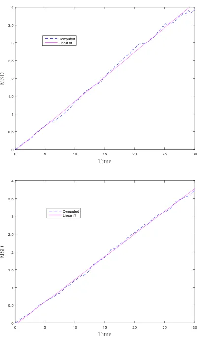
No-flow simulations are also conducted to compute the diffusivity of the DPD/sDPD fluid for a wide range of the Schmidt number, namely (10,20,_{· · ·} ,90,100,200,_{· · ·},1000). The imposed viscosities are chosen near their upper limits. Variations of the mean squared displacement of the particles against time can be well approximated by polynomials of first order. Some typical results of the diffusivity are displayed in Figure 4. For Sc0 = 400 and

η0 = 49, the self-diffusion coefficient is estimated as 0.0346 by the proposed sDPD and 0.0319

by the proposed DPD, which are comparable to the value of 0.0306 predicted by the kinetic theory.

Figure 5 displays the computed Sc against the imposed value Sc0 in the log-scale coordinate

system by the three methods. It can be seen that values of the Schmidt number predicted by the kinetic theory very much agree with the computed (and specified) values as expected; the formulation is doing its job well. The computed Sc values by the proposed sDPD and

DPD are in good agreement with the kinetic theory predictions, particularly for the proposed DPD. It is noted that the error bars associated with the data points are not displayed here since their values are quite small in comparison with the coordinate scale used.

6

Concluding remarks

discretisation) in terms of computational effort and ability to yield a stable viscosity from different imposed shear rates.

References

1. P.J. Hoogerbrugge, J.M.V.A. Koelman, Simulating microscopic hydrodynamic phe-nomena with dissipative particle dynamics, Europhysics Letters. 19(3) (1992) 155-160.

2. C. Marsh, Theoretical aspect of dissipative particle dynamics (PhD Thesis), University of Oxford, 1998.

3. P. Espa˜nol, P. Warren, Statistical mechanics of dissipative particle dynamics, Euro-physics Letters. 30(4) (1995) 191-196.

4. P. Espa˜nol, Hydrodynamics from dissipative particle dynamics, Phys. Rev. E. 52 (1995) 1734-1742.

5. J.H. Irving, J.G. Kirkwood, The statistical mechanical theory of transport processes. IV. The equations of hydrodynamics, J. Chem. Phys. 18 (1950) 817-829.

6. R.M. F¨uchslin, H. Fellermann, A. Eriksson, H.-J. Ziock, Coarse graining and scaling in dissipative particle dynamics, J. Chem. Phys. 130 (2009) 214102.

7. Y. Kong, C.W. Manke, W.G. Madden, A.G. Schlijper, Effect of solvent quality on the conformation and relaxation of polymers via dissipative particle dynamics, J. Chem. Phys. 107 (1997) 592.

8. E.S. Boek, P.V. Coveney, H.N.N. Lekkerkerker, P. van der Schoot, Simulating the rheology of dense colloidal suspensions using dissipative particle dynamics, Phys. Rev. E. 55(3) (1997) 3124-3133.

9. N. Phan-Thien, Understanding Viscoelasticity: An Introduction to Rheology, second Edition, Springer-Verlag, Berlin, 2013.

10. P. Espa˜nol, M. Revenga, Smoothed dissipative particle dynamics, Phys. Rev. E. 67(2) (2003) 026705.

11. W. Pan, B. Caswell, G.E. Karniadakis, Rheology, microstructure and migration in Brownian colloidal suspensions, Langmuir. 26(1) (2010) 133-142.

12. N. Phan-Thien, N. Mai-Duy, B.C. Khoo, A spring model for suspended particles in dissipative particle dynamics, J. Rheol. 58 (2014) 839-867.

13. N. Mai-Duy, N. Phan-Thien, B.C. Khoo, Investigation of particles size effects in Dis-sipative Particle Dynamics (DPD) modelling of colloidal suspensions, Comput. Phys. Comm. 189 (2015) 37-46.

14. X. Bian, S. Litvinov, R. Qian, M. Ellero, N.A. Adams, Multiscale modeling of particle in suspension with smoothed dissipative particle dynamics, Phys. Fluids. 24 (2012) 012002.

16. R.D. Groot, P.B. Warren, Dissipative particle dynamics: Bridging the gap between atomistic and mesoscopic simulation, J. Chem. Phys. 107 (1997) 4423.

17. V. Symeonidis, G.E. Karniadakis, B. Caswell, Schmidt number effects in dissipative particle dynamics simulation of polymers, J. Chem. Phys. 125 (2006) 184902.

18. X.J. Fan, N. Phan-Thien, S. Chen, X. Wu, T.Y. Ng, Simulating flow of DNA suspension using dissipative particle dynamics, Phys. Fluids. 18(6) (2006) 063102.

19. C.A. Marsh, G. Backx, M.H. Ernst, Static and dynamic properties of dissipative par-ticle dynamics, Phys. Rev. E. 56(2) (1997) 1676-1691.

20. S. Litvinov, M. Ellero, X. Hu, N.A. Adams, Self-diffusion coefficient in smoothed dis-sipative particle dynamics, J. Chem. Phys. 130 (2009) 021101.

21. X.Y. Hu, N.A. Adams, Angular-momentum conservative smoothed particle dynamics for incompressible viscous flows, Phys. Fluids. 18 (2006) 101702.

22. J.J. Monaghan, Smoothed particle hydrodynamics, Reports on Progress in Physics. 68(8) (2005) 1703.

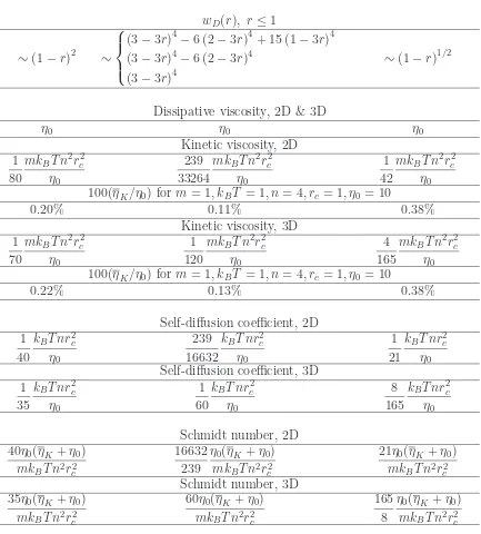
Table 1: Diffusivity, viscosity and Schmidt number predicted by kinetic theory for sDPD

Lucy Quintic Proposed (s= 1/2)

wD(r), r≤1

∼(1₋r)2 _∼



 

 

(3₋3r)4₋6 (2₋3r)4+ 15 (1₋3r)4 (3₋3r)4₋6 (2₋3r)4

(3₋3r)4

∼(1₋r)1/2

Dissipative viscosity, 2D & 3D

η0 η0 η0

Kinetic viscosity, 2D 1

80

mkBT n2r2c

η0

239 33264

mkBT n2r2c

η0

1 42

mkBT n2r2c

η0

100(η_K/η0) for m= 1, kBT = 1, n = 4, rc = 1, η0 = 10

0.20% 0.11% 0.38%

Kinetic viscosity, 3D 1

70

mkBT n2r2c

η0

1 120

mkBT n2r2c

η0

4 165

mkBT n2rc2

η0

100(η_K/η0) for m= 1, kBT = 1, n = 4, rc = 1, η0 = 10

0.22% 0.13% 0.38%

Self-diffusion coefficient, 2D 1

40

kBT nr2c

η0

239 16632

kBT nrc2

η0

1 21

kBT nr2c

η0

Self-diffusion coefficient, 3D 1

35

kBT nr2c

η0

1 60

kBT nrc2

η0

8 165

kBT nrc2

η0

Schmidt number, 2D 40η0(η_K+η0)

mkBT n2rc2

16632 239

η0(η_K +η0)

mkBT n2r2c

21η0(η_K+η0)

mkBT n2rc2

Schmidt number, 3D 35η0(η_K+η0)

mkBT n2rc2

60η0(η_K +η0)

mkBT n2r2c

165 8

η0(η_K+η0)

Table 2: Couette flow, rc = 2.5, m = 1, kBT = 1, n = 4: Variation in the computed viscosity η∗

over a range of shear rate (0.05, 0.1, 0.2, 0.5, 1). Note that η0 is the input viscosity, η the viscosity by the kinetic theory and η∗

the viscosity obtained from numerical simulation, where the shear stress is calculated using the Irving-Kirkwood formula. The proposed function/kernel consistently outperforms the Lucy and quintic kernels. However, solutions by the proposed sDPD are still less stable than those by the proposed DPD.

η0 = 10

Method η η∗

mean(η∗

) std(η∗

)

sDPD (Lucy) 10.1250 8.9345 9.7711 9.9974 10.3299 10.5475 9.9161 0.6247

sDPD (quintic) 10.0718 8.7544 9.2305 9.6393 10.2517 10.6194 9.6991 0.7530

Proposed sDPD (s= 1/2) 10.2381 10.0224 9.9574 10.3460 10.6081 10.7689 10.3406 0.3547 Proposed DPD (s= 1/2) 10.2381 10.0457 10.0344 10.2302 10.1977 10.1982 10.1412 0.0934

η0 = 50

Method η η∗

mean(η∗

) std(η∗

)

sDPD (Lucy) 50.0250 45.3252 46.9274 48.1738 49.4448 50.1124 47.9967 1.9290

sDPD (quintic) 50.0144 41.7764 44.3180 46.5540 48.7942 49.9483 46.2782 3.3160 Proposed DPD (s= 1/2) 50.0476 48.0100 48.9023 49.6504 50.1365 50.5073 49.4413 1.0003 Proposed sDPD (s= 1/2) 50.0476 49.2684 49.3672 49.3490 49.2771 49.1392 49.2802 0.0899

Table 3: Couette flow, rc = 1, η0 = 10, m = 1, kBT = 1, n = 4, 200000 time steps: Variation in the computed viscosity η∗

over a range of shear rate (0.05, 0.1, 0.2, 0.5, 1). Note that η0 is the input viscosity, η the viscosity by the kinetic theory and η∗

the viscosity obtained from simulation, where the shear stress is calculated using the Irving-Kirkwood formula. With rc = 1, the proposed DPD is able to produce reasonable (constant) values of viscosity, probably owing to the fact that DPD is a coarse-grained model. In contrast, the sDPD fails to represent a fluid properly as the SPH discretisation (rc = 1, n= 4) used for the pressure gradient term appears too coarse.

Methood η0 η η∗

mean(η∗

) std(η∗

)

sDPD (Lucy) 10 10.0200 5.3589 6.7573 8.2504 10.4305 11.6631 8.4920 2.5835

Proposed DPD (s= 1/2) 10 10.0381 9.3215 9.3359 9.3162 9.3038 9.2621 9.3079 0.0281

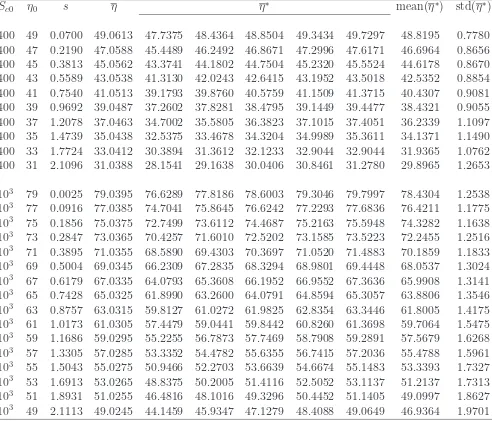
Table 4: Couette flow, the proposed sDPD method with η and Sc as specified inputs, rc =

2.5, m= 1, kBT = 1, n= 4: Variation in the computed viscosity η∗ over a range of shear rate

(0.05, 0.1, 0.2, 0.5, 1). Note thatη0is the input viscosity, ηthe viscosity by the kinetic theory

andη∗

the viscosity obtained from numerical simulation, where the shear stress is calculated using the Irving-Kirkwood formula. The differences between the mean computed viscosity and the viscosity by the kinetic theory are in the range of 0.4% to 3.6% for Sc0 = 400, and

of 0.7% to 4.2% for Sc0 = 1000. These values are small in comparison to the error within

10₋30% by the standard DPD reported in [16].

Sc0 η0 s η η

∗

mean(η∗

) std(η∗

)

400 49 0.0700 49.0613 47.7375 48.4364 48.8504 49.3434 49.7297 48.8195 0.7780 400 47 0.2190 47.0588 45.4489 46.2492 46.8671 47.2996 47.6171 46.6964 0.8656 400 45 0.3813 45.0562 43.3741 44.1802 44.7504 45.2320 45.5524 44.6178 0.8670 400 43 0.5589 43.0538 41.3130 42.0243 42.6415 43.1952 43.5018 42.5352 0.8854 400 41 0.7540 41.0513 39.1793 39.8760 40.5759 41.1509 41.3715 40.4307 0.9081 400 39 0.9692 39.0487 37.2602 37.8281 38.4795 39.1449 39.4477 38.4321 0.9055 400 37 1.2078 37.0463 34.7002 35.5805 36.3823 37.1015 37.4051 36.2339 1.1097 400 35 1.4739 35.0438 32.5375 33.4678 34.3204 34.9989 35.3611 34.1371 1.1490 400 33 1.7724 33.0412 30.3894 31.3612 32.1233 32.9044 32.9044 31.9365 1.0762 400 31 2.1096 31.0388 28.1541 29.1638 30.0406 30.8461 31.2780 29.8965 1.2653

103

79 0.0025 79.0395 76.6289 77.8186 78.6003 79.3046 79.7997 78.4304 1.2538 103

77 0.0916 77.0385 74.7041 75.8645 76.6242 77.2293 77.6836 76.4211 1.1775 103

75 0.1856 75.0375 72.7499 73.6112 74.4687 75.2163 75.5948 74.3282 1.1638 103

73 0.2847 73.0365 70.4257 71.6010 72.5202 73.1585 73.5223 72.2455 1.2516 103

71 0.3895 71.0355 68.5890 69.4303 70.3697 71.0520 71.4883 70.1859 1.1833 103

69 0.5004 69.0345 66.2309 67.2835 68.3294 68.9801 69.4448 68.0537 1.3024 103

67 0.6179 67.0335 64.0793 65.3608 66.1952 66.9552 67.3636 65.9908 1.3141 103

65 0.7428 65.0325 61.8990 63.2600 64.0791 64.8594 65.3057 63.8806 1.3546 103

63 0.8757 63.0315 59.8127 61.0272 61.9825 62.8354 63.3446 61.8005 1.4175 103

61 1.0173 61.0305 57.4479 59.0441 59.8442 60.8260 61.3698 59.7064 1.5475 103

59 1.1686 59.0295 55.2255 56.7873 57.7469 58.7908 59.2891 57.5679 1.6268 103

57 1.3305 57.0285 53.3352 54.4782 55.6355 56.7415 57.2036 55.4788 1.5961 103

55 1.5043 55.0275 50.9466 52.2703 53.6639 54.6674 55.1483 53.3393 1.7327 103

53 1.6913 53.0265 48.8375 50.2005 51.4116 52.5052 53.1137 51.2137 1.7313 103

51 1.8931 51.0255 46.4816 48.1016 49.3296 50.4452 51.1405 49.0997 1.8627 103

Table 5: Couette flow, the proposed DPD method with η and Sc as specified inputs, rc =

2.5, m= 1, kBT = 1, n= 4, 200000 time steps: Variation in the computed viscosity η∗ over a

range of shear rate (0.05, 0.1, 0.2, 0.5, 1). Note thatη0 is the input viscosity, ηthe viscosity

by the kinetic theory and η∗

the viscosity obtained from numerical simulation, where the shear stress is calculated using the Irving-Kirkwood formula. The differences between the mean computed viscosity and the viscosity by the kinetic theory are in the range of 0.8% to 4.1% for Sc0 = 400, and of 1.0% to 4.6% for Sc0 = 1000. These values are small in

comparison to the error within 10₋30% by the standard DPD reported in [16].

Sc0 η0 s η η

∗

mean(η∗

) std(η∗

)

400 49 0.0700 49.0613 48.6527 48.6499 48.6072 48.5680 48.5020 48.5960 0.0630 400 47 0.2190 47.0588 46.5280 46.5480 46.5677 46.5308 46.4424 46.5234 0.0480 400 45 0.3813 45.0562 44.4845 44.5760 44.5253 44.4635 44.3705 44.4840 0.0766 400 43 0.5589 43.0538 42.4420 42.4700 42.5166 42.3820 42.2749 42.4171 0.0932 400 41 0.7540 41.0513 40.4706 40.3918 40.4173 40.3121 40.2135 40.3611 0.1003 400 39 0.9692 39.0487 38.3384 38.3526 38.3091 38.2067 38.1076 38.2629 0.1039 400 37 1.2078 37.0463 36.3077 36.3432 36.1828 36.1117 35.9647 36.1820 0.1533 400 35 1.4739 35.0438 34.1004 34.1354 34.1335 33.9547 33.8340 34.0316 0.1331 400 33 1.7724 33.0412 32.0159 31.9489 31.9399 31.7961 31.6702 31.8742 0.1394 400 31 2.1096 31.0388 29.8289 29.9010 29.8028 29.6245 29.4874 29.7289 0.1690

103

79 0.0025 79.0395 78.2694 78.3023 78.2876 78.1766 77.9877 78.2047 0.1308 103

77 0.0916 77.0385 76.3450 76.2902 76.3054 76.1304 75.9391 76.2020 0.1682 103

75 0.1856 75.0375 74.2632 74.3087 74.1706 74.0582 73.8520 74.1305 0.1829 103

73 0.2847 73.0365 72.2327 72.2330 72.1074 71.9916 71.7881 72.0706 0.1871 103

71 0.3895 71.0355 70.1473 70.1546 70.0979 69.9238 69.6816 70.0010 0.2015 103

69 0.5004 69.0345 67.9465 68.0606 68.0470 67.8259 67.6197 67.8999 0.1828 103

67 0.6179 67.0335 66.0183 66.0046 65.9752 65.7646 65.5433 65.8612 0.2053 103

65 0.7428 65.0325 63.9088 63.9030 63.8650 63.6619 63.4285 63.7534 0.2079 103

63 0.8757 63.0315 61.8891 61.9422 61.7653 61.5269 61.3271 61.6901 0.2585 103

61 1.0173 61.0305 59.9201 59.8296 59.6849 59.4454 59.2193 59.6199 0.2869 103

59 1.1686 59.0295 57.7898 57.8112 57.5797 57.3167 57.0336 57.5062 0.3310 103

57 1.3305 57.0285 55.6375 55.6135 55.4978 55.1821 54.8979 55.3658 0.3183 103

55 1.5043 55.0275 53.3698 53.5036 53.3964 53.0487 52.7674 53.2172 0.3034 103

53 1.6913 53.0265 51.4842 51.3216 51.1973 50.8794 50.5953 51.0956 0.3569 103

51 1.8931 51.0255 49.3580 49.1922 49.0333 48.7463 48.4186 48.9497 0.3728 103

1 1.5 2 2.5 3 3.5 4 4.5 5 1

2 3 4 5 6 7

rc

η

/η

0

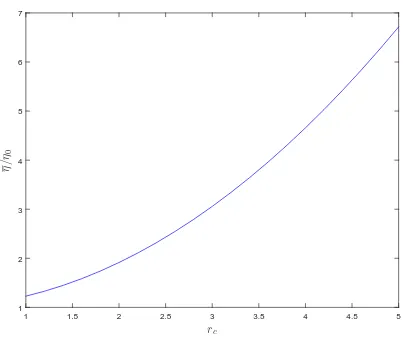
Figure 1: Kinetic theory, Lucy kernel, m= 1, kBT = 1, n= 4, η0 = 1, low Schmidt numbers

0 0.1 0.2 0.3 0.4 0.5 0.6 0.7 0.8 0.9 1 0

0.05 0.1 0.15 0.2 0.25 0.3 0.35 0.4 0.45

Lucy Quintic Proposed (s=1/2)

r/rc

W

0 0.1 0.2 0.3 0.4 0.5 0.6 0.7 0.8 0.9 1 0

0.005 0.01 0.015 0.02 0.025 0.03

Lucy Quintic Proposed (s=1/2)

r/rc

wD

y

-5 -4 -3 -2 -1 0 1 2 3 4 5

-1 0 1 2 3 4 5

n T u

x

u

y

y

-5 -4 -3 -2 -1 0 1 2 3 4 5

-2 0 2 4 6 8 10

Shear stress Normal stress difference

Figure 3: Couette flow, m = 1, kBT = 1, η0 = 10, shear rate of 1, 200000 time steps: results

0 5 10 15 20 25 30 0

0.5 1 1.5 2 2.5 3 3.5 4

Computed Linear fit

Time

M

S

D

0 5 10 15 20 25 30

0 0.5 1 1.5 2 2.5 3 3.5 4

Computed Linear fit

Time

M

S

D

Figure 4: Proposed kernel, m = 1, kBT = 1, n = 4, rc = 2.5, Sc0 = 400, η0 = 49: the mean

101 102 103 101

102 103

Kinetic theory Proposed sDPD Proposed DPD

Imposed Sc

C

om

p

u

te

d

Sc

Figure 5: Proposed kernel, m = 1, kBT = 1, n = 4, rc = 2.5: Computed Schmidt numbers