www.atmos-chem-phys.net/17/3573/2017/ doi:10.5194/acp-17-3573-2017
© Author(s) 2017. CC Attribution 3.0 License.
HEPPA-II model–measurement intercomparison project:
EPP indirect effects during the dynamically perturbed
NH winter 2008–2009
Bernd Funke1, William Ball2, Stefan Bender4, Angela Gardini1, V. Lynn Harvey5, Alyn Lambert6,
Manuel López-Puertas1, Daniel R. Marsh7, Katharina Meraner8, Holger Nieder4, Sanna-Mari Päivärinta3,9,
Kristell Pérot10, Cora E. Randall5, Thomas Reddmann4, Eugene Rozanov2,11, Hauke Schmidt8, Annika Seppälä3, Miriam Sinnhuber4, Timofei Sukhodolov2, Gabriele P. Stiller4, Natalia D. Tsvetkova12, Pekka T. Verronen3, Stefan Versick4,14, Thomas von Clarmann4, Kaley A. Walker13, and Vladimir Yushkov12
1Instituto de Astrofísica de Andalucía, CSIC, Apdo. 3004, 18008 Granada, Spain
2Physikalisch-Meteorologisches Observatorium, World Radiation Center, Davos, Switzerland 3Earth Observation Unit, Finnish Meteorological Institute, Helsinki, Finland
4Karlsruhe Institute of Technology (KIT), Institute of Meteorology and Climate Research (IMK-ASF), P.O. Box 3640,
76021 Karlsruhe, Germany
5Laboratory for Atmospheric and Space Physics, University of Colorado, Boulder, USA 6Jet Propulsion Laboratory, California Institute of Technology, Pasadena, California, USA 7National Center for Atmospheric Research, Boulder, Colorado, USA
8Max Planck Institute for Meteorology, Hamburg, Germany 9Department of Physics, University of Helsinki, Helsinki, Finland 10Chalmers University of Technology, Göteborg, Sweden
11Institute for Atmospheric and Climate Science ETH, Zurich, Switzerland 12Central Aerological Observatory, Moscow, Russia
13Department of Physics, University of Toronto, Toronto, Ontario, Canada
14Karlsruhe Institute of Technology (KIT), Steinbuch Centre for Computing (SCC), Karlsruhe, Germany
Correspondence to:Bernd Funke ([email protected])
Received: 2 November 2016 – Discussion started: 9 December 2016
Revised: 14 February 2017 – Accepted: 22 February 2017 – Published: 14 March 2017
Abstract.We compare simulations from three high-top (with upper lid above 120 km) and five medium-top (with upper lid around 80 km) atmospheric models with observations of odd nitrogen (NOx =NO + NO2), temperature, and carbon
monoxide from seven satellite instruments (ACE-FTS on SciSat, GOMOS, MIPAS, and SCIAMACHY on Envisat, MLS on Aura, SABER on TIMED, and SMR on Odin) dur-ing the Northern Hemisphere (NH) polar winter 2008/2009. The models included in the comparison are the 3-D chem-istry transport model 3dCTM, the ECHAM5/MESSy Atmo-spheric Chemistry (EMAC) model, FinROSE, the Hamburg Model of the Neutral and Ionized Atmosphere (HAMMO-NIA), the Karlsruhe Simulation Model of the Middle
At-mosphere (KASIMA), the modelling tools for SOlar Cli-mate Ozone Links studies (SOCOL and CAO-SOCOL), and the Whole Atmosphere Community Climate Model (WACCM4). The comparison focuses on the energetic parti-cle precipitation (EPP) indirect effect, that is, the polar winter descent of NOxlargely produced by EPP in the mesosphere
boundary condition obtained from MIPAS observations has further been applied to medium-top models. Most models provide a good representation of the mesospheric tracer de-scent in general, and the EPP indirect effect in particular, during the unperturbed (pre-SSW) period of the NH win-ter 2008/2009. The observed NOx descent into the lower
mesosphere and stratosphere is generally reproduced within 20 %. Larger discrepancies of a few model simulations could be traced back either to the impact of the models’ grav-ity wave drag scheme on the polar wintertime meridional circulation or to a combination of prescribed NOx mixing
ratio at the uppermost model layer and low vertical reso-lution. In March–April, after the ES event, however, mod-elled mesospheric and stratospheric NOx distributions
de-viate significantly from the observations. The too-fast and early downward propagation of the NOx tongue,
encoun-tered in most simulations, coincides with a temperature high bias in the lower mesosphere (0.2–0.05 hPa), likely caused by an overestimation of descent velocities. In contrast, upper-mesospheric temperatures (at 0.05–0.001 hPa) are generally underestimated by the high-top models after the onset of the ES event, being indicative for too-slow descent and hence too-low NOxfluxes. As a consequence, the magnitude of the
simulated NOxtongue is generally underestimated by these
models. Descending NOx amounts simulated with
medium-top models are on average closer to the observations but show a large spread of up to several hundred percent. This is pri-marily attributed to the different vertical model domains in which the NOxupper boundary condition is applied. In
gen-eral, the intercomparison demonstrates the ability of state-of-the-art atmospheric models to reproduce the EPP indi-rect effect in dynamically and geomagnetically quiescent NH winter conditions. The encountered differences between ob-served and simulated NOx, CO, and temperature
distribu-tions during the perturbed phase of the 2009 NH winter, how-ever, emphasize the need for model improvements in the dy-namical representation of elevated stratopause events in or-der to allow for a better description of the EPP indirect effect under these particular conditions.
1 Introduction
The potential impact of energetic particle precipitation (EPP) on regional climate is nowadays becoming recognized. Solar forcing recommendations for the recently launched Climate Model Intercomparison Project Phase 6 (Eyring et al., 2016) include, for the first time, the consideration of energetic par-ticle effects (Matthes et al., 2016). EPP is strongly linked to solar activity and hence to the solar cycle, either directly by coronal mass ejections producing sporadically large fluxes of solar energetic particles or indirectly by the quasi-continuous impact of the solar wind on the Earth’s magnetosphere. In the mesosphere and lower thermosphere (MLT), EPP-induced
ionization initiates the production of odd nitrogen and odd hydrogen (the latter below∼85 km), both of them destroying ozone via catalytic cycles. Odd nitrogen (NOx=NO + NO2)
is long-lived during polar winter and is then regularly trans-ported down from its source region into the stratosphere to altitudes well below 30 km (e.g. Randall et al., 2007; Funke et al., 2014a). This so-called EPP indirect effect contributes significant amounts of NOx to the polar middle atmosphere
during each winter. EPP-induced ozone changes are thought to modify the thermal structure and winds in the stratosphere which, in turn, modulate the strength of the Arctic polar vortex. The introduced signal could then propagate down to the surface, introducing significant variations of regional cli-mate, particularly in the Northern Hemisphere (NH) (Seppälä et al., 2009; Baumgaertner et al., 2011; Rozanov et al., 2012; Seppälä and Clilverd, 2014; Maliniemi et al., 2014).
At present, many chemistry climate models account for EPP-induced ionization and its chemical impact on the neu-tral atmosphere, which is required for the simulation of at-mospheric EPP effects and ultimately for the investigation of potential EPP–climate links. A comprehensive evaluation of these models’ capacity to reproduce observed EPP effects by means of coordinated intercomparison studies is a necessary step towards this goal. The High Energy Particle Precipita-tion in the Atmosphere (HEPPA) model vs. data intercom-parison initiative (Funke et al., 2011) evaluated the chemi-cal response of nitrogen and chlorine species in nine atmo-spheric models to the “Halloween” solar proton event in late October 2003 with observations taken by the Michelson In-terferometer for Passive Atmospheric Sounding (MIPAS) on Envisat. Reasonable agreement of observed and modelled re-active nitrogen and ozone changes was found, demonstrating the models’ overall ability to reproduce the direct EPP effect by solar protons. However, most models failed to adequately describe the repartitioning of nitrogen compounds in the af-termath of the event which could be attributed to deficien-cies in the representation of the D-region ion chemistry and motivated recent model developments (Egorova et al., 2011; Verronen et al., 2016; Andersson et al., 2016).
The observation-based evaluation of the simulated at-mospheric effects of magnetospheric particles, which are thought to be of higher relevance for climate, is more chal-lenging because of the quasi-continuous flux of electrons compared to protons and the difficulty in separating between local production and downward transport of NOx during
polar winter. Although a pronounced dependence of reac-tive nitrogen enhancements in the polar winter stratosphere and mesosphere on the geomagnetic activity levels has been demonstrated (Funke et al., 2014b), dynamical variability, particularly in the NH, can mask out this effect. In partic-ular, the occurrence of elevated stratopause (ES) events fol-lowing sudden stratospheric warmings (SSWs) during Arctic winters often causes much larger mesospheric NOx
vortex during the SSW. The ability of climate models to ade-quately simulate tracer transport in Arctic winters, including perturbed winters characterized by SSW and ES events, is therefore crucial to accurately model EPP effects and their possible NH regional climate impacts.
Simulations of mesospheric tracer descent during dynam-ically perturbed NH winters have been compared with ob-servations in several studies. Using the KArlsruhe SImu-lation Model of the middle Atmosphere (KASIMA) with specified dynamics below 48 km and prescribed NOx
con-centrations from MIPAS night-time NO2observations above
55 km, Reddmann et al. (2010) calculated the amount of EPP-NOxentering the stratosphere from July 2002 to March
2004. KASIMA reproduced the MIPAS observations of NOx
entering the stratosphere reasonably well, even during the SSW winter 2003/2004. However, the ability of the model to adequately simulate mesospheric tracer transport could not be tested because of the constrained NOxin the mesosphere.
Salmi et al. (2011) and Päivärinta et al. (2016), in turn, used FinROSE with constrained NOxat the upper boundary
(∼80 km) for both early 2009 and 2012. Their results show that FinROSE is able to qualitatively reproduce the down-ward descent of NOx from the MLT region into the
strato-sphere, but the actual NOx amounts can differ significantly
from the observations. In the case of chemical transport mod-els (CTMs), the results are strongly affected by the meteoro-logical data, i.e. a source of uncertainty, used to drive the model. McLandress et al. (2013) used a version of the Cana-dian Middle Atmosphere Model (CMAM) that was nudged toward reanalysis data up to 1 hPa to examine the impacts of parameterized orographic and non-orographic gravity wave drag (GWD) on the zonal mean circulation of the mesosphere during the perturbed NH winters 2006 and 2009 in compar-ison with temperature and carbon monoxide (CO) observa-tions from the Microwave Limb Sounder (MLS) on Aura. They found that non-orographic GWD is primarily respon-sible for driving the circulation that results in the descent of CO from the thermosphere following the warmings. Randall et al. (2015) investigated the NOx descent during the
Arc-tic winter/spring of 2004 with Whole Atmosphere Commu-nity Climate Model (WACCM) simulations that were nudged to Modern-Era Retrospective Analysis for Research and Ap-plications (MERRA) data. They found that their simulated NOx, although qualitatively reproducing the enhanced
de-scent after the ES event, was up to a factor of 5 too low com-pared with satellite observations. This underestimation was attributed to missing NO production by high-energy elec-trons in the mesosphere in combination with an underesti-mation of mesospheric descent during the recovery phase af-ter the SSW. Siskind et al. (2015) compared simulations of mesospheric tracer descent in the winter and spring of 2009 with two versions of WACCM, one constrained with data from MERRA, which extends up to 50 km, and the other constrained to the Navy Operational Global Atmospheric Prediction System-Advanced Level Physics High Altitude
(NOGAPS-ALPHA), which extends up to 92 km. By com-parison with Solar Occultation for Ice Experiment (SOFIE) data they showed that constraining WACCM to NOGAPS-ALPHA yields a dramatic improvement in the simulated de-scent of enhanced NOxand very low methane.
Most of these studies suggest that the model representation of the perturbed dynamics during NH winters with SSWs and ES events has a crucial impact on the simulated amount of NOx transported into the stratosphere and that a proper
parameterization of unresolved GWD is key to achieving agreement with observations. However, previous studies fo-cused on individual models, making it difficult to assess the overall ability of state-of-the-art atmospheric models to re-produce the EPP indirect effect in NH winters. Comprehen-sive multi-model intercomparisons addressing dynamically perturbed NH winters, however, have so far been restricted to the assessment of the temperature zonal mean, planetary wave, and tidal variability during the 2009 SSW event in the middle and upper atmosphere (Pedatella et al., 2014), as well as to the impacts on the ionosphere variability (Pe-datella et al., 2016). Further, although our knowledge of tem-perature and tracer distributions in polar winters has dramat-ically increased with the advent of atmospheric satellite ob-servations, specific intercomparisons and validation efforts focussing on such conditions are sparse. A systematic assess-ment of this knowledge is therefore essential to quantitatively diagnose the model performance with respect to mesospheric tracer transport under perturbed (and unperturbed) polar win-ter conditions.
A coordinated intercomparison project focussing on tracer descent and the EPP indirect effect during such a winter was therefore initiated in the frame of the SPARC/WCRP’s SOLARIS-HEPPA activity. In this so-called HEPPA-II project, simulations of the NH polar winter 2008/2009 from eight atmospheric models have been compared with ob-servations of temperature and concentrations of NOx and
compari-son are the 3-D chemistry transport model (3dCTM), the ECHAM5/MESSy Atmospheric Chemistry (EMAC) model, FinROSE, the Hamburg Model of the Neutral and Ionized Atmosphere (HAMMONIA), KASIMA, the modelling tools for SOlar Climate Ozone Links studies (SOCOL and CAO-SOCOL), and WACCM (Version 4). Only three of these models (3dCTM, HAMMONIA, and WACCM) extend up into the lower thermosphere where a large fraction of EPP-induced odd nitrogen production occurs. All other models have their upper lid in the mesosphere and require an odd ni-trogen upper boundary condition (UBC), accounting for EPP production higher up, for simulating the introduced EPP in-direct effect in the model domain. This UBC has been con-structed from NOx observations of the MIPAS instrument
taken during the Arctic winter 2008–2009. The chemistry climate model simulations have been nudged toward reanal-ysis data below 1 hPa while being unconstrained above. The restriction of specified dynamics to the stratosphere is a com-promise that is hoped to provide a realistic evolution of meso-spheric meteorology by upward control, while still allow-ing for the assessment of self-generated tracer descent in the models.
In this study we report results from the HEPPA-II inter-comparison project. A major aim is the identification and characterization of model biases and their uncertainties in the simulations of the perturbed 2008/2009 NH winter by systematically comparing to the suite of satellite observa-tions. For this purpose, common diagnostics are applied in all comparisons, and the sampling characteristics of the in-struments are taken into account. Since the study focusses on the evaluation of the ability of the models to simulate the source and transport of MLT tracers by means of observed quantities (i.e. temperature and trace gas abundances), any more sophisticated analysis, e.g. qualifying the different GW drag parameterizations, is outside the scope of this compar-ison. However, our analysis should motivate such studies to identify the deficits in key processes of this vertical coupling. The paper is organized as follows: Sect. 2 gives an overview on the satellite observations and data products used in this study. Section 3 describes the participating chemistry climate and transport models. The NOx UBC employed in
the medium-top models is described in Sect. 4, and Sect. 5 introduces the intercomparison method. Results of the inter-comparisons are discussed in Sect. 6 with focus on the rep-resentation of the EPP indirect effect by the high-top mod-els in the upper mesosphere and lower thermosphere and, in Sect. 7, with focus on the upper-stratospheric and meso-spheric representation in all models.
2 Satellite observations 2.1 ACE-FTS/SciSat
The ACE-FTS has performed infrared solar occultation mea-surements from the SciSat satellite since February 2004 (Bernath et al., 2005). The SciSat satellite is in a highly in-clined circular orbit (74◦) and thus provides measurements from 85◦N to 85◦S over each year with a significant focus on polar measurements. Up to 30 measurements are made each day by ACE-FTS, extending from the cloud tops to
∼150 km. ACE-FTS observations of temperature, CO, and NOx during Arctic ES winters have been analysed in
sev-eral previous studies (e.g. Randall et al., 2009, 2015). Here, version 3.0 of the ACE-FTS dataset was used, which covers 21 February 2004 to 30 September 2010. The ACE-FTS re-trieval algorithm is described in Boone et al. (2005) and the specific details of version 3.0/3.5 are provided in Boone et al. (2013). NOxis provided from ACE-FTS using the retrieved
NO (6–107 km) and NO2(7–52 km) profiles. Above 52 km,
where both sunset and sunrise NO2concentrations are very
small and hence not detectable, the scaled a priori NO2
pro-file has been used to extend the NOx profiles to the higher
altitudes. The CO profiles extend from 5 to 110 km and tem-perature is retrieved from 15 to 125 km. The vertical resolu-tion of the ACE-FTS measurements is∼3 km, based on the instrument field of view (Boone et al., 2005).
The version 3.5 NO profiles differ from HALOE by−15 to
+6 % between 27 and 53 km and from summertime MIPAS measurements by−9 to+2 % between 36 and 52 km (Sheese et al., 2016a). For NO2, the bias found between ACE-FTS
and a suite of other limb and occultation sounders is better than 18 % from 17 to 27 km and−15 % from 28 to 41 km (Sheese et al., 2016a). For both of these species, a box model was used to apply a diurnal scaling to the ACE-FTS profiles before the comparisons. ACE-FTS CO has been compared with MIPAS and MLS by Sheese et al. (2016b). On average, there is a−11 % bias between 28 and 50 km with respect to MIPAS and a bias of±10 %. Based on comparisons with co-incident satellite observations (within 350 km and 3 h), it has been found that ACE-FTS v3.5 temperatures agree to within
±2 K between 15 and 40 km, within±7 K between 40 and 80 km, and within±12 K between 80 and 100 km (P. Sheese, personal communication, 2016).
2.2 GOMOS/Envisat
O2, and aerosols in the middle atmosphere. Here, we have
used GOMOS NO2profiles (version GOPR_6.0c_6.0f)
mea-sured in night-time conditions (solar zenith angle at tangent point location>107◦; solar zenith angle at spacecraft loca-tion>90◦to avoid stray light). The altitude range for NO2
in non-polar conditions is 20–50 km and extends up to 70 km in polar winter when enhanced amounts of NO2are present
in the atmosphere (Seppälä et al., 2007; Hauchecorne et al., 2007). The typical precision of the NO2measurements is 5–
20 % while the systematic error of the NO2observations is
estimated to be of the order of few percent (1–5 %) (Tammi-nen et al., 2010; Verro(Tammi-nen et al., 2009). Vertical resolution is 4 km (Kyrölä et al., 2010). As NO is quickly converted into NO2 by reaction with O3 after sunset, the night-time
GO-MOS NO2measurements used here are a reasonable
repre-sentation of stratospheric and lower mesospheric NOx.
Because stars are used as the light source, the locations of the observations change with time. A representative distri-bution of the latitudes sampled during the course of a year can be seen in Figs. 7–9 of Bertaux et al. (2010). Due to this sampling, for the NH polar region in winter 2008–2009, GOMOS night-time NO2observations were available for the
period of December 2008–January 2009. GOMOS measure-ments provide the constituent profiles as number densities. For the purpose of this study these were converted to vol-ume mixing ratios (VMRs) using temperature and pressure profiles from the WACCM model (see below).
2.3 MIPAS/Envisat
The MIPAS instrument (Fischer et al., 2008) on Envisat pro-vided global stratospheric and mesospheric measurements of temperature (García-Comas et al., 2014), NO and NO2
(Funke et al., 2014a), CO (Funke et al., 2009), as well as nu-merous other trace species (e.g. von Clarmann et al., 2009, 2013) during 2002–2012. Here, we use observations taken in the nearly continuous nominal observation mode (scanning range 6–70 km, hereinafter referred to as MIPAS-NOM), as well as occasional special mode observations (middle and upper-atmospheric observation modes covering 20–100 and 40–170 km, respectively, hereinafter referred to as MIPAS-UA), the latter taken with a frequency of about 1 out of 5 days. We also use special mode UA observations which include three orbits per day passing the 20◦W–70◦E and 160◦E–110◦W sectors during 14–18 and 21–27 January 2009 and which were taken as support for the Dynamics and Energetics of the Lower Thermosphere in Aurora 2 (DELTA-2) campaign (Abe et al., 2006).
MIPAS-NOM NOx data have been built from NO and
NO2data versions V5r_NO_220 and V5r_NO2_220,
respec-tively. MIPAS-UA NOx data are based on data versions
V4o_NO_501/611 and V4o_NO2_501/600. In the middle-to high-latitude polar winters, typical vertical resolutions are 4–6 km below 50 km and 6–9 km above, while the single measurement precision is on the order of 5–15 %.
System-atic errors, dominated by non-local thermodynamic equilib-rium (non-LTE) uncertainties of NO and NO2, have been
es-timated to be less than 10 %. CO data (version V5r_CO_220) used here have a single measurement precision ranging from 20–30 % above 45 km to 70–80 % in the lower stratosphere. The vertical resolution is 6–12 km. The single measure-ment precision of temperature data (versions v5r_T_220 and v5r_T_521/621 for MIPAS-NOM and MIPAS-UA, respec-tively) is 0.5–2 K below 70 km and 2–7 K above. The system-atic error is typically 1–3 K below 85 km and 3–11 K above. The average vertical resolution is 3–6 km below 90 km and 6–10 km above.
2.4 MLS/Aura
The MLS instrument (Waters et al., 2006) was launched on 15 July 2004 and measures thermal microwave emission from Earth’s limb. On each day MLS provides∼3500 verti-cal profiles of temperature and trace gases between 82◦S and 82◦N spaced∼1.5◦apart along great circles following the orbit track. Manney et al. (2009) employed MLS data version 3.2 to analyse tracer transport during the Arctic ES winter 2006. Here, we use version 4.2 temperature and CO. Temper-ature is deemed useful for scientific studies between 316 and 0.001 hPa. The vertical resolution is 5 km near 40 km and in-creases to∼10 km near 90 km (Livesey, 2016). In the meso-sphere, systematic and random errors are 2.5 K and compar-isons with correlative measurements show a 0–7 K cold bias (Schwartz et al., 2008). CO is recommended for scientific use from 215 to 0.0046 hPa (Pumphrey et al., 2007). The vertical resolution is 4–5 km in the stratosphere and 6–7 km in the mesosphere. Froidevaux et al. (2006) indicate that the CO data have a 25–50 % positive bias in the mesosphere. Esti-mates of absolute accuracy are 10 % (Filipiak et al., 2005). For this work, temperature and CO data have been filtered using the precision, status, quality, and convergence values provided by the MLS science team (Livesey, 2016).
2.5 SABER/TIMED
errors are <1.5 K below 75 km, 4 K at 85 km, and 5 K at 100 km (Remsberg et al., 2008; García-Comas et al., 2008). The vertical resolution is about 2 km. A thorough comparison of these temperatures with those measured by other satel-lites, MIPAS, ACE-FTS, MLS, OSIRIS, SOFIE, and by li-dar measurements has been recently carried out by García-Comas et al. (2014) in a study about the validation of MIPAS vM21 temperatures. The comparison of SABER v2.0 with MIPAS vM21 is remarkably good, with differences smaller than 2 K at all altitudes and seasons, except for high-latitude summers above 65 km where they are 3–4 K at 65–80 km (MIPAS colder) and 5–7 K around the mesopause (MIPAS warmer).
2.6 SMR/Odin
The SMR instrument is a limb emission sounder aboard Odin, a Swedish-led satellite launched in 2001 in cooper-ation with the Canadian, French, and Finnish space agen-cies (Murtagh et al., 2002). Odin is orbiting the Earth in a sun-synchronous orbit at an initial altitude of 580 km and at Equator-crossing times varying between 06:00 and 07:00 local time for the morning overpass (18:00 and 19:00 lo-cal time fore the evening overpass). These parameters are slightly changing with time due to the drifting orbit. SMR is measuring globally a variety of trace gases and the temper-ature from the upper troposphere to the lower thermosphere (Merino et al., 2002).
Nitric oxide is retrieved from the observation of thermal emission lines in a band centred around 551.7 GHz. The ver-sion 2.1 of NO data is used in this study. The overall verti-cal coverage is from 7 to 115 km, and in the altitude range considered here the vertical resolution is about 7 km (Pérot et al., 2014). NO data are available approximately 4 days per month after 2007, on an irregular basis of 2 observation days in a 14-day cycle. Systematic errors amount to 3 % from spectroscopic parameters, 2 % from calibration, and 3–6 % from sideband suppression (Sheese et al., 2013). The single measurement retrieval error amounts to 44–48 %, in the case of Antarctic night-time mesosphere–lower thermosphere, as studied by Sheese et al. (2013). A comparison study per-formed by Bender et al. (2015) showed that SMR NO mea-surements were consistent with NO meamea-surements by SCIA-MACHY, MIPAS, and ACE-FTS despite the different mea-surement methods and retrieval strategies used for these four instruments.
2.7 SCIAMACHY/Envisat
The SCIAMACHY (see Burrows et al., 1995; Bovensmann et al., 1999) is a limb-sounding UV–VIS–NIR spectrometer on Envisat. Among the main measurement modes, the nom-inal limb mode carried out limb measurements from ground to 105 km until mid-October 2003, and after 15 October 2003 up to 91 km. From July 2008 until April 2012, SCIAMACHY
carried out a special mesosphere–lower thermosphere mode (MLT), scanning from 50 to 150 km for 1 day every 2 weeks. Nitric oxide is retrieved from the NO gamma bands (UV channel 1, 230–314 nm) (Bender et al., 2013, 2017) in the 60–160 km range using a tomographic approach. The re-trieval from the MLT mode yields the NO number densities with a vertical resolution of 5–10 km between 70 and 150 km. With the nominal mode, the same resolution is achieved between 65 and 80 km. The average single orbit measure-ment error amounts to about 30 %. Systematic errors amount to 7 % from uncertain spectroscopic data, 3 % from uncer-tainties in the solar spectrum (Chance and Kurucz, 2010), and about 10 % from temperature uncertainties. Because the NO gamma bands are fluorescent emissions, the retrieval of NO is restricted to daylight observations. Polar winter data are therefore restricted to latitudes equatorward of the polar night terminator (around 70◦in the mesosphere–lower
ther-mosphere at winter solstice).
The retrieved NO number densities from the MLT mode have been compared to ACE-FTS, MIPAS, and SMR (Ben-der et al., 2015). The measurements were found to be con-sistent among all instruments with SCIAMACHY retrieving slightly lower densities compared to the other instruments during polar winter but higher values in mesospheric polar summer and mid-to-low latitudes.
3 Chemistry climate models
In the following, the participating atmospheric models are described and details on the set-up of the simulations are provided. Since the dynamical evolution in the mesosphere is strongly constrained by the behaviour of the lower atmo-sphere, particularly during a perturbed NH winter, model simulations have been either nudged to or rely entirely on meteorological reanalysis data in order to allow for compar-isons to observations. High-top models, having their upper lid above 120 km and including explicit schemes for consid-eration of NOxproduction by particle-induced ionization, are
described in Sect. 3.1. Medium-top models, having their up-per lid around 80 km, are described in Sect. 3.2. These mod-els applied a common odd nitrogen UBC in order to account for EPP production above the model domain (see Sect. 4). A summary of the different model settings and characteristics is given in Table 1.
3.1 High-top models 3.1.1 3dCTM
the LIMA general circulation model (Berger, 2008), and the model upper boundary is defined by the availability of these data. For the version used here, LIMA is nudged to (1◦×1◦)
ECMWF operational data with a constant nudging of temper-ature, zonal and meridional winds between the surface and 35 km, and a linear decrease in nudging strength to 45 km, the upper limit of the nudging area. No parameterization of the GWD is implemented either in LIMA or in 3dCTM. Only waves with horizontal scales of≥500 km and a temporal res-olution of 2–12 h are represented Berger (2008). A compar-ison of momentum flux climatologies provided in Fig. 7 of Berger (2008) with common GWD schemes as shown, e.g. in Fig. 5 of Holton and Zhu (1984), shows that the gravity wave momentum flux in the mesosphere is underestimated by LIMA by about a factor of 2–3 in both the summer and winter hemisphere. In the winter hemisphere, the vertical structure of the GW momentum flux is also somehow dif-ferent; while Holton and Zhu (1984) essentially show one broad peak at∼65–95 km altitude, varying in strength from
−80 to 120 ms−1d−1, the LIMA profile shows a double peak structure with a broad peak of −40–60 ms−1d−1 at∼70– 90 km altitude, a minimum in 90–100 km, and a secondary peak above 100 km. This means that the vertical downward motion throughout the mesosphere will be underestimated during winter.
The model chemistry scheme has been adapted from the original SLIMCAT code for use in the mesosphere and lower thermosphere as described in Sinnhuber et al. (2012): the model considers the photolysis of O2, CO2, CH4, and H2O
in the far-UV wavelength range down to the Lymanαline. Also, in the mesosphere and lower thermosphere, chemi-cal families are not considered for NOx and Ox species,
and H2O, O2, and H2 are now integrated as active
chemi-cal species in the model. Additionally, parameterizations for the impact of atmospheric ionization from particle impact and photoionization are considered based on ion-chemistry model studies (Nieder et al., 2014). The photoionization rate is based on the parameterization of Solomon and Qian (2005); particle impact ionization rates are prescribed using the four-dimensional field provided by the AIMOS model (Wissing and Kallenrode, 2009) version 1.2. Model data are output every 15 min and interpolated onto the satellite geolo-cations from this.
3.1.2 HAMMONIA
HAMMONIA is an upward extension of the ECHAM5 at-mospheric general circulation model (Roeckner et al., 2006). The model’s dynamics and radiation are fully coupled to the chemical Model of Ozone and Related Tracers (MOZART, Kinnison et al., 2007). A detailed description of the model is given by Schmidt et al. (2006). To simulate the effects of EPP, HAMMONIA is modified to incorporate the ion chemistry of the E and F region as described in Kieser (2011) and Meraner and Schmidt (2016). The ion chemistry
treats 5 ion–electron recombinations and 12 ion-neutral reac-tions including 50 neutral and 6 charged (O+, O+
2, N
+, N+
2,
NO+, e−) components. Additionally, five reactions directly
involving energetic particles are considered. The correspond-ing reaction rates are calculated uscorrespond-ing the particle-induced ionization rates provided by Atmospheric Ionization Mod-ule Osnabrück (AIMOS version 1.6) (Wissing and Kallen-rode, 2009). The explicit simulation of energetic particle ef-fects on chemistry is limited to above 10−3hPa, whereas be-low this altitude the production of N(2D), N(4S), and HOx
is parameterized following Jackman et al. (2005a). Photo-chemistry includes six reactions involving radiation at wave-lengths shorter than Lyman-α. Therefore the parameteriza-tion of Solomon and Qian (2005) and the observed 10.7 cm solar radio flux is used. Orographic gravity waves are pa-rameterized according to Lott and Miller (1997), while non-orographic gravity waves are parameterized according to the Doppler-spread theory from Hines (1997). A geographically uniform isotropic gravity wave source spectrum with a con-stant root-mean-square (RMS) wave wind speed of 0.8 m s−1 launched at 830 hPa is used. Additional to the homogeneous source of gravity waves, HAMMONIA considers the gen-eration of gravity waves from tropospheric fronts following Charron and Manzini (2002). At locations where frontoge-nesis occurs the gravity wave spectrum is launched with an RMS wave wind speed of 2 m s−1 instead of 0.8 m s−1. A more detailed description of the gravity wave scheme used in HAMMONIA is given in Meraner et al. (2016). Note also that this setting of the gravity wave parameters differs from the simulation of the same winter analysed in Pedatella et al. (2014) where the waves were launched at about 650 hPa and no frontal sources were used. Sea surface temperature and sea ice cover are taken from the Atmospheric Model Inter-comparison Project 2 (AMIP2) climatology. Output is pro-vided every 2 h and afterwards interpolated to the satellite geolocations. The model is nudged from 850 to 1 hPa with an upper and lower transition zone to the 6-hourly values of the ERA-Interim reanalysis data (Dee et al., 2011). The “spin-up” time is 1 year starting on 1 January 2008.
3.1.3 WACCM
Table 1.Summarized description of the atmospheric models involved in this study.
High-top Vertical Horizontal Vert. res. Meteorological data Family Kinetic EPP-NOx
model domain (km) resolution (km) nudginga approacha datab production
3dCTM ∼10–150 2.5◦×3.75◦ ∼1–3 LIMA (ECMWF<1 hPa) no S06 AIMOS 1.2
HAMMONIA ∼0–250 1.9◦×1.9◦ ∼3 ERA-I (<1 hPa) no S06 AIMOS 1.6
WACCM ∼0–140 1.9◦×2.5◦ ∼1.5 MERRA (<50 km) no S11 auroral prod.
Medium-top NOxUBC
model range (hPa)
CAO-SOCOL ∼0–80 3.75◦×3.75◦ ∼2 ERA-I (<1 hPa) no S06 0.01
FinROSE ∼0–80 6◦×3◦ ∼2–7 ECMWF (whole model domain) no S06 0.03–0.01
KASIMA ∼7–120 2.8◦×2.8◦ 0.75–3.8 ERA-I (<1 hPa) no S03 0.03
EMAC ∼0–80 2.8◦×2.8◦ ∼1–4 ERA-I (<0.2 hPa) reduced S11 0.09–0.01
SOCOL ∼0–80 2.8◦×2.8◦ ∼2 ERA-I (<1 hPa) no S11 0.01
aSee model descriptions in Sect. 3 for details.
bS11: Sander, S. P. et al. (2011); S03: Sander et al. (2003); S06: Sander et al. (2006)
free-running between 50 km and the model top at approxi-mately 140 km (4.5×10⁻⁶hPa). Heating rates and photoly-sis are calculated using observed daily solar spectral irradi-ance based on the empirical model of Lean et al. (2005) and geomagnetic activity effects in the auroral region are param-eterized in terms of the Kp index (Marsh et al., 2007). The standard WACCM chemistry is described and evaluated ex-tensively in WMO (2010). Reaction rates are from Sander, S. P. et al. (2011). For these simulations we have modified the N+N2 reaction to include two additional pathways as
described in Funke et al. (2008). It should be noted that both WACCM and HAMMONIA use the same chemical solver based on the MOZART3 chemistry (Kinnison et al., 2007), include the same set of ionized species, and use the parame-terized EUV ionization rates from Solomon and Qian (2005). For these simulations the latter parameterization has been ex-tended to include the photoionization of CO2 in the EUV.
Above 5×10⁻⁴hPa (∼100 km) ionization from electrons is calculated by the WACCM parameterized aurora. It is as-sumed that 1.25 N atoms are produced per ion pair and di-vide the N atom production between ground state, N(4S), at 0.55 per ion pair and excited state, N(2D), at 0.7 per ion pair (Jackman et al., 2005b; Porter et al., 1976). This simulation followed the “REFC1D” protocol of the Chemistry Climate Model Initiative (Eyring et al., 2013) for the specification of time-dependent greenhouse gases and ozone-depleting sub-stances. WACCM constituent and temperature profiles were saved at the model grid point and time step (model time step is 30 min) closest to each of the MIPAS observation loca-tions. Eddy diffusion created by the dissipation of parame-terized gravity waves in WACCM depends on the value as-sumed for the Prandtl number,Pr, which describes the ratio of the eddy momentum flux to the eddy flux of potential tem-perature or chemical species. In these simulationsP r=4, as in the study of Garcia et al. (2014).
3.2 Medium-top models 3.2.1 CAO-SOCOL
Since HEPPA-I (Funke et al., 2011) the CCM SOCOL (mod-elling tool for studies SOlar Climate Ozone Links) has been upgraded to version 3 with substantial changes related to the advection of the species. These changes and the detailed eval-uation of the new version performance were documented by Stenke et al. (2013). The CCM SOCOL v.3 consists of the MEZON chemistry transport model (Egorova et al., 2003) and MA-ECHAM5, the middle atmosphere version of the ECHAM general circulation model (Roeckner et al., 2006). Dynamical and physical processes in SOCOL are calculated every 15 min within the model, while full radiative and chem-ical calculations are performed every 2 h. Chemchem-ical con-stituents are transported using a flux-form semi-Lagrangian scheme (Lin and Rood, 1996), and the chemical solver is based on a Newton–Raphson iterative method taking into account 41 chemical species, 140 gas-phase reactions, 46 photolysis reactions, and 16 heterogeneous reactions. The CCM SOCOL v.3 was installed in CAO (Central Aerolog-ical Observatory, Moscow, Russian Federation) and modi-fied to use assimilation of the meteorological fields from the ERA-I reanalysis, which is necessary to reproduce the con-sidered SSW and ES events in January 2009. The model is nudged from 850 to 1 hPa using the Jeuken et al. (1996) approach. Orographic gravity waves are parameterized ac-cording to Lott and Miller (1997). Non-orographic gravity waves are parameterized using Hines (1997) scheme imple-mented to ECHAM5 with a constant RMS wave wind speed of 1.0 m s−1 introduced at 830 hPa for all geographical lo-cations. The daily mean NOx mixing ratio at 0.01 hPa from
MIPAS measurements (see Sect. 4) was used as the UBC at the uppermost model layer. The NOx mixing ratio was
model for any particular time step at the second layer from the model top. Model output was interpolated in time and space to the provided satellite geolocations.
3.2.2 EMAC
The EMAC model is a numerical chemistry and climate simulation system that includes submodels describing tro-pospheric and middle atmosphere processes and their in-teraction with oceans, land, and human influences (Jöckel et al., 2010). It uses the second version of the Modular Earth Submodel System (MESSy2) to link multi-institutional computer codes. The core atmospheric model is the fifth-generation European Centre Hamburg general circulation model (ECHAM5, Roeckner et al., 2006). For the present study we applied EMAC (ECHAM5 version 5.3.02, MESSy version 2.50) in the T42L90MA resolution. The model is nudged to ERA-Interim reanalysis data from the surface to 0.2 hPa (with decreasing nudging strength in the transition region in the five levels above) using the nudging coefficients suggested in Jeuken et al. (1996). The UBC for NOx is
pre-scribed in the top four layers (0.01 to 0.09 hPa) of the model. For gravity waves we used the submodel GWAVE which con-tains the original Hines non-orographic gravity wave routines (Hines, 1997) from ECHAM5 in a modularized structure. We tuned the parameter rmscon (RMS wind speed at bottom launch level of 642.9 hPa), which controls the dissipation of gravity waves, to 0.8 m s−1. For gas-phase reactions we used the submodel MECCA (Sander, R. et al., 2011) and for pho-tolysis the submodel JVAL (Sander et al., 2014). Included were 110 gas-phase reactions and 44 photolysis reactions. The NOxfamily was reduced to NO and NO2. The chemical
tracers were initialized from a multi-annual EMAC model run. Model output was done for each time step (10 min) which afterwards was interpolated to the satellite geoloca-tions.
3.2.3 FinROSE
FinROSE is a global 3-D CTM (further developed model ver-sion of the one described by Damski et al., 2007). The model dynamics for the whole model domain is forced with external meteorological data, whereas the vertical wind is calculated inside the model by using the continuity equation. In this study FinROSE is nudged with ECMWF operational analysis data. This means that changes in the atmospheric composi-tion do not affect the model dynamics, and gravity wave pa-rameterization is included already in the meteorological forc-ing data. FinROSE reproduces the distributions of 41 species from the stratosphere up to the mesosphere and lower ther-mosphere and also includes about 120 homogeneous reac-tions and 30 photodissociation processes. Photodissociation frequencies are calculated using a radiative transfer model (Kylling et al., 1997). In addition to homogeneous chemistry, the model also includes heterogeneous chemistry, i.e.
forma-tion and sedimentaforma-tion of polar stratospheric clouds (PSCs) and reactions on PSCs. The model is designed for middle at-mospheric studies and thus the chemistry is not defined in the troposphere, but the tropospheric abundances are given as boundary conditions. For this study, the UBC for NOx
(i.e. NO + NO2) was implemented in the MLT region at about
0.03–0.01 hPa (the top two model layers). Output in the satel-lite geolocations was composed already during the model run by finding the closest model grid point and time step to every geolocation.
3.2.4 KASIMA
The KASIMA model is a 3-D mechanistic model of the mid-dle atmosphere including full midmid-dle atmosphere chemistry (Kouker et al., 1999). The model can be coupled to specific meteorological situations by using analysed lower boundary conditions and nudging terms for vorticity, divergence, and temperature. Here the version used for the HEPPA-I experi-ment has been applied (Funke et al., 2011) but with a hori-zontal resolution of about 2.8◦×2.8◦(T42). The frequency of output is every 6 h. The model is nudged to ERA-Interim analyses below 1 hPa. A numerical time step of 6 min was used in the experiments. The model uses a Lindzen-type pa-rameterization (Holton, 1982) to include the effect of break-ing gravity waves, but no specific parameterization of oro-graphic gravity waves. Further details of the model are found in Funke et al. (2011). The UBC for NOx was set at the
0.3 hPa level, and not above. This occasionally causes de-viations between the observations and the model above this level.
3.2.5 SOCOL
The applied version of the CCM SOCOL improves upon CAO-SOCOL and was prepared for participation in the IGBP/SPARC CCMI project. The tropospheric chemistry component was extended by adding the Mainz Isoprene Mechanism (MIM-1), which comprises 16 organic species and a further 44 chemical reactions (Pöschl et al., 2000). The cloud influence on photolysis rates was introduced us-ing a cloud modification factor (Chang et al., 1987). Inter-active lightning source of NOxwas introduced following the
Price and Rind (1992) approach and adopting local scaling factors based on satellite measurements. The kinetic con-stants and absorption cross sections were updated following Sander, S. P. et al. (2011). The new parameterization of the UV heating rates (Sukhodolov et al., 2014) as well as NOx
and HOx production by energetic particles (Rozanov et al.,
2012) was adopted. For HEPPA-II the model was run with T42 horizontal resolution, which corresponds approximately to 2.8◦×2.8◦, and 39 vertical levels between the ground and 0.01 hPa. The nudging set-up and UBC for NOxare the same
✵✵✵ ✵✵✁ ✵✂✵ ✵✂✁ ✵✄✵ ✵✄✁ ✵☎✵
◆
✆
✝
✞
✟
✠
✡
☛
☛
✟
✞
☞
❆✌ ✍
▼✎✏❆✑ ✒✓ ✔ ▼
▼✎✏❆✑ ✒✕❆ ✑ ▼❙
✂✓✶✖ ✄✵✵✷
✂✗ ✘✙ ✄✵✵✷
✂✚ ✛✜ ✄✵✵✢
✂✣ ✘✤ ✄✵✵✢
✂▼✛ ✥ ✄✵✵✢
✂❆ ✦✥ ✄✵✵✢ ✻✧
✼✧ ✽✧ ✾✧
★
✩
✪
✫
✬
✪
✭
✮
✯
✰
✩
✱
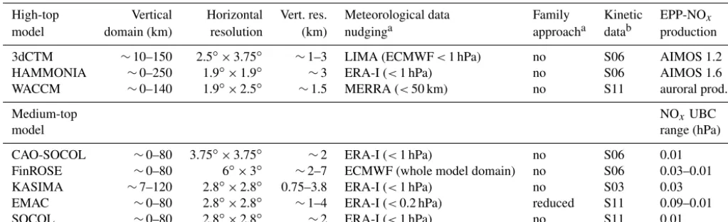
[image:10.612.128.465.61.231.2]✲
Figure 1.Upper panel: daily averaged NOx mixing ratios from satellite observations (open squares) at 0.022 hPa within 60–90◦N (black
is MIPAS-NOM, blue is MIPAS-UA, red is SMR/Odin, green is ACE-FTS) and those of the upper boundary condition (filled diamonds) sampled at the respective observations’ time and location. Lower panel: mean latitude averaged over all observations of the individual instruments within 60–90◦N. All averages are area-weighted.
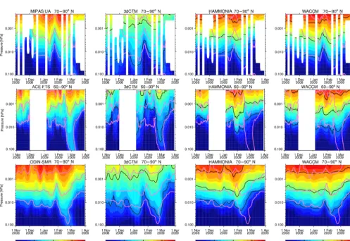
Figure 2.Observed and modelled NOxVMRs of MIPAS and ACE (upper two rows) and NO of SMR (lower row) in NH polar MLT region
[image:10.612.51.548.295.636.2]4 NOx UBC for medium-top models
The UBC for NOx mixing ratio has been constructed from
MIPAS-NOM observation data versions v4o_NO_200 and v4o_NO2_200 by projecting individual observations onto a regular grid in longitude, latitude, pressure level, and time with daily cadence using a distance-weighting algorithm. All observations taken within±12 h time difference,±10◦ lat-itude, and ±25◦ longitude have been considered at each grid point (weighted by the inverse distance squared) and have been vertically interpolated to a fixed pressure grid. Data gaps in space and time have been filled by linear in-terpolation. Note that in the model–measurement intercom-parisons a newer version of MIPAS NOx is used, which
was not available when the UBC was generated prior to the model runs. The horizontal resolution of the NOx UBC
is 1.25◦×2.5◦(latitude×longitude). Thirteen vertical pres-sure levels within 1–0.01 hPa are covered to allow for inter-polation to the respective upper lid of the models. The NOx
UBC has been evaluated by comparing with available satel-lite observations (see Fig. 1). To avoid sampling errors in the comparisons, the UBC field has been sampled at the mea-surements’ locations of each day before averaging over the polar cap region. In general, there is very good agreement (within 10–20 %) with independent NOxobservations.
How-ever, larger differences up to 20–50 % occur sporadically for observations close to the vortex edge (e.g. when comparing to ACT-FTS at the end of February) where horizontal gradi-ents are very pronounced.
5 Intercomparison strategy
The discrete horizontal sampling of satellite observations can cause large uncertainties in intercomparisons of observed and modelled averaged quantities, particularly if the sampling is sparse, irregular, or variable in time (Toohey et al., 2013). To reduce the impact of sampling errors, we follow the same approach that was successfully applied in the first HEPPA intercomparison study (Funke et al., 2011): the model output has been sampled at the locations and times of the individual observations and has been vertically interpolated to the ob-served pressure levels. If available (i.e. in the case of MIPAS and MLS), averaging kernels have been applied to the model results as described in Funke et al. (2011). Profiles have only been considered in the vertical range where the instruments’ sensitivity is high enough to provide meaningful data; the remaining profile regions have been excluded in both obser-vations and model results.
Model–measurement comparisons were performed on ba-sis of daily and/or quasi-monthly averaged zonal mean data, which have been calculated in the same way for both observations and simulations. For most comparisons, data have been further binned within 70–90◦N, applying area-conserving (cos(θ )) weights. Note, however, that the
sam-pled portion of this latitude bin varies from instrument to in-strument, making a direct comparison of the observational results difficult. However, the comparison of model biases with respect to different observational datasets is mostly un-affected. The binning has been extended to 60–90◦N in the comparisons to ACE-FTS data in order to allow for evalua-tions prior to February 2009. We recall that ACE-FTS has a discrete but time-varying latitude coverage (see Fig. 1) such that the resulting averages represent only a small fraction of the entire bin.
6 Upper mesosphere and lower thermosphere
In this section NOx, CO, and temperature fields of the
high-top models 3dCTM, HAMMONIA, and WACCM are com-pared to the observations in the MLT, the source region of odd nitrogen produced by EPP. Although, strictly speaking, temperature is not a tracer of vertical motion, the adiabatic warming during periods of strong descent introduces observ-able changes of the thermal structure of this region which can be used as diagnostics of vertical transport in the models. The simultaneous evaluation of modelled NOx, CO, and
temper-ature distributions allows then to attribute model biases to deficiencies in the simulation of either particle-induced NOx
production or of dynamics.
Figure 2 shows the vertical distribution of NH polar NOx
over time in the simulations and MIPAS-UA, ACE-FTS, and ODIN-SMR observations at 0.1 to 2×10⁻⁴hPa. SCIA-MACHY observations of NO densities have not been in-cluded in this figure because NH polar observations are only available after the beginning of February. Note that MIPAS-UA and ACE-FTS provided NOx VMRs, while SMR
ob-served NO VMR only. This, however, introduces differences only below approximately 0.01 hPa since NOx is entirely
in the form of NO above. The comparisons with the three instruments provide a consistent picture of model biases. While WACCM and HAMMONIA reproduce the observa-tions fairly well during the whole time period in the up-per mesosphere and lower thermosphere (above the 0.01 hPa level), 3dCTM exhibits too small NOx abundances in this
vertical region. Below the 0.01 hPa level and during the pre-SSW phase of the winter (November–January), WACCM and HAMMONIA agree well with the observations while 3dCTM overestimates NOx in this vertical region during
most of the pre-SSW phase.
The SSW event starts with the breakdown of the polar vor-tex, and the dilution of the mesospheric NOx by upwelling
and increased horizontal mixing. This is clearly observed by MIPAS and SMR as a decrease of NOxbetween roughly 0.01
and 0.001 hPa. This initial NOxdecrease is captured well by
WACCM and 3dCTM, though it is too weak in the HAMMO-NIA simulation. The initial decrease of NOxduring the SSW
is followed by strong downwelling of NOxleading to a
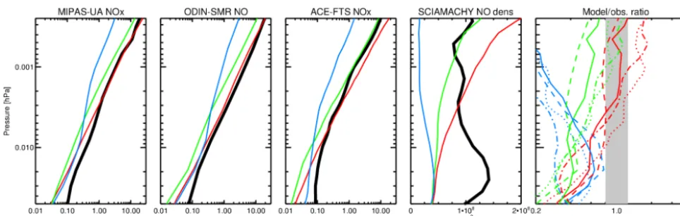
Figure 3.Comparison of observed polar mid-winter NOxmean profiles (thick black lines) a to 3dCTM (blue), HAMMONIA (green), and
WACCM (red). Right panel: ratio of model results and MIPAS-UA (solid), SMR/Odin (dashed), and ACE-FTS (dotted) observations. The grey shaded area indicates the±25 % range. Data have been averaged over 70–90◦N and 5 December 2008–12 January 2009 (60–90◦N and 5 November 2008–12 January 2009 in the case of ACE-FTS).
of the characteristic NOx“tongue”. This is qualitatively
cap-tured by all models, however, the amount of NOxtransported
into the lower mesosphere (below 0.01 hPa) is significantly underestimated. The timing of the onset of the enhanced de-scent varies considerably among the models and, compared to the observations, occurs slightly too early in HAMMO-NIA and too late in 3dCTM. The onset of ES-related NOx
in-creases in WACCM coincides with the observed onset, how-ever, the modelled increases appear to last for a shorter time.
6.1 Unperturbed early (pre-SSW) phase
In the following, the observed and modelled vertical structure of NOx, CO, and temperature during mid-winter (pre-SSW
phase) is analysed in more detail to evaluate the models’ abil-ity to reproduce the EPP indirect effect for unperturbed con-ditions. Figure 3 compares the observed and modelled NOx
mid-winter mean profiles averaged over 70–90◦N and 5 De-cember 2008–15 January 2009 (60–90◦N and 5 November 2008–15 January 2009 in the case of ACE-FTS) above the al-titude of 0.05 hPa. The observed vertical structure of NOxis
reasonably well reproduced by HAMMONIA and WACCM during this period. Differences with respect to the observa-tions are mostly within 20–50 %, with WACCM being over-all more on the high side and HAMMONIA more on the low side (particularly at altitudes below 0.002 hPa). As dis-cussed earlier, the 3dCTM simulations show a much less pro-nounced vertical gradient resulting in a significant (in terms of the observational spread) NOx underestimation (up to a
factor of 8) at altitudes above 10−2hPa and overestimation (up to a factor of 3) below. Figure 4 compares the correspond-ing mean profiles of CO, observed by MIPAS-UA, MLS, and ACE-FTS above the altitude of 0.5 hPa. Again, WACCM and HAMMONIA show a vertical gradient that is roughly in agreement with the observations. In contrast, the
abso-lute CO values of WACCM are slightly (up to 40 %) higher while HAMMONIA underestimates the CO abundances by a factor of 2–3. The latter can be explained by missing ther-mospheric production mechanisms in the model, specifically the CO2photolysis in the extreme ultraviolet (at wavelengths
<121 nm) and the reaction of CO2with the atomic oxygen
ion (Garcia et al., 2014), that act in addition to the photolysis of CO2 in Lyman-alpha and the Schumann–Runge
contin-uum. The 3dCTM simulations, similarly as for NOx, show a
gradient in the mesosphere that is too weak compared to the observations, resulting in an underestimation above 0.03 hPa and an overestimation below. The corresponding tempera-ture profiles (see Fig. 5), observed by MIPAS-UA, MLS, and ACE-FTS (note that SABER is not included because the observations in December cover only up to 52◦N) indi-cate good agreement with the observations for HAMMONIA and a slight warm bias of 5–10 K for WACCM. Mesospheric 3dCTM temperatures are systematically too cold by 10–30 K in the middle and lower mesosphere.
The good overall agreement of NOx, CO, and
tempera-ture from HAMMONIA and WACCM with the observations in December suggests that both NOxsources and dynamical
conditions are well represented by these models, allowing for an adequate description of the EPP indirect effect in the MLT during unperturbed conditions early in NH winters. Interest-ingly, the consideration of ionization induced by mid-energy electron in HAMMONIA (via AIMOS) does not introduce noticeable differences in the NO distribution with respect to WACCM, the latter only accounting for auroral electrons. This suggests that the impact of mid-energy electron during the solar minimum 2008/2009 NH winter was rather small. 3dCTM simulations, in contrast, show significant discrepan-cies with the observations. The similarity of the model bias in the vertical gradients of NOx and CO suggests that these
Figure 4.Comparison of observed polar mid-winter CO mean profiles (thick black lines) to 3dCTM (blue), HAMMONIA (green), and WACCM (red). Right panel: ratio of model results and MIPAS-UA (solid), MLS (dashed), and ACE-FTS (dotted) observations. The grey shaded area indicates the±25 % range. Data have been averaged over 70–90◦N and 5 December 2008–12 January 2009 (60–90◦N and 5 November 2008–12 January 2009 in the case of ACE-FTS).
Figure 5.Comparison of observed polar mid-winter temperature mean profiles (thick black lines) to 3dCTM (blue), HAMMONIA (green), and WACCM (red). Right panel: temperature difference of the simulations and MIPAS-UA (solid), MLS (dashed), and ACE-FTS (dotted) observations. The grey shaded area indicates the±5 K range. Data have been averaged over 70–90◦N and 5 December 2008–12 January 2009 (60–90◦N and 5 November 2008–12 January 2009 in the case of ACE-FTS).
representation of dynamics in 3dCTM rather than to the EPP source. The vertical gradient of the 3dCTM CO and NOx
profiles both show values in the lower thermosphere that are too low and values in the upper to mid-mesosphere that are too high. The underestimation of lower thermospheric CO is likely due to the model chemistry as, like in HAMMO-NIA, neither the EUV photolysis of CO2nor the production
of CO by positive ion chemistry in the lower thermosphere are considered in 3dCTM. The underestimation of thermo-spheric NOx could be caused by a too-weak NO production
or too-fast transport out of the (polar) source region, either by horizontal mixing or across the mesopause. The high val-ues of both CO and NOx in the mesosphere, however, are
likely due to the representation of mesospheric dynamics in 3dCTM, which is driven by temperatures and wind fields from the LIMA model. A likely reason seems the neglect
of subscale (≤500 km) gravity waves in the LIMA model, leading to an underestimation of the GW drag throughout the mesosphere but to an overestimation in the lowermost thermosphere (see Sect. 2.7). This leads to a suppression of vertical motion in the mesosphere, which is also reflected in a negative bias in temperatures, and, consequently, to an ac-cumulation of CO and NOx.
6.2 Perturbed late (post-SSW) phase
Figure 6 compares the observed and modelled NOx
Febru-ary mean profiles corresponding to the perturbed post-SSW phase of this winter, characterized by enhanced descent of NOx. This comparison includes also SCIAMACHY NO
Figure 6.Comparison of observed NOxmean profiles (thick black lines) for February 2009 (during the ES event) and 70–90◦N to 3dCTM
(blue), HAMMONIA (green), and WACCM (red). Right panel: ratio of model results and MIPAS-UA (solid), SMR/Odin (dashed), ACE-FTS (dotted), and SCIAMACHY (dash-dotted) observations. The grey shaded area indicates the±25 % range. Data have been averaged over 70–90◦N and 1 February–1 March 2009 (60–90◦N and 1 February 2008–15 March 2009 in the case of ACE-FTS).
likely related to the enhanced spatial and temporal variabil-ity. On average, however, these differences are very similar to those encountered during mid-winter. Below 0.005 hPa, all models systematically underestimate the observed NOx
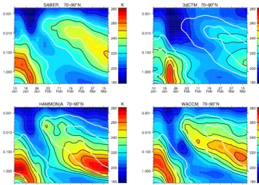
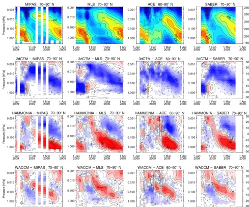
in-creases associated with the ES event by a factor of 2–3. Adiabatic heating associated with the enhanced meso-spheric descent is responsible for the reformation of the stratopause at a pressure level as high as 0.005 hPa. Fig-ure 7 shows the temporal evolution of the vertical tempera-ture structempera-ture at 70–90◦N in January–March as observed by
SABER and simulated by 3dCTM (LIMA), HAMMONIA, and WACCM. We have chosen this observational dataset for the comparison to the models because of its full temporal coverage in this period and the high vertical resolution in the entire vertical range. The observed elevated stratopause started to develop at the beginning of February and remained at around 0.01 hPa for a month before it descended to its climatological height in the course of March. The high-est stratopause temperatures during the elevated phase were reached around 20 February. Although all models simulate an elevated stratopause, its temporal evolution differs signif-icantly from the observations. HAMMONIA and WACCM show an ES onset and formation level similar to the ob-served ones, but highest temperatures at this level are reached immediately after the onset, about 20 days earlier than in the observations. In both models, the ES level starts to de-scend immediately after its formation, more quickly than ob-served and faster in HAMMONIA than in WACCM. During the descent, the modelled stratopauses become increasingly warmer. 3dCTM, in contrast, simulates a much later onset (about 2 weeks after the observed one) and the ES temper-atures are much colder than in the observations. However, the modelled ES remains at an elevated level for a longer time (although slightly lower than the observed ES) and the time delay until reaching the maximum ES temperatures is comparable to the observed temperature evolution. These
dif-ferences between 3dCTM on the one hand and WACCM, HAMMONIA, and mostly also the observations on the other hand highlight the role of subscale gravity waves for the temporal evolution of the ES event. The onset of the SSW event is driven mainly by large-scale planetary waves break-ing down the horizontal circulation and is captured compar-atively well by all three models. However, the reformation of the stratopause at upper-mesospheric altitudes is driven by small-scale gravity waves reaching up to the upper meso-sphere after the event. As these smaller gravity waves are essentially missing in the LIMA data, the build-up of the el-evated stratopause is delayed in 3dCTM, and its strength is weaker.
To investigate whether the encountered differences be-tween the models and SABER data are robust with respect to instrumental uncertainties, we extend the analysis to MIPAS-UA, ACE, and MLS temperature observations and compare the model differences to all observations (see Fig. 8). Despite minor changes related to the different latitude range covered by the instruments, the encountered model biases are consis-tent for all instruments, indicating a too-cold mesosphere of 3dCTM and a dipole-type pattern in HAMMONIA and, less pronounced, in WACCM with colder temperatures after the ES onset in the upper mesosphere and warmer temperatures below.
Figure 7. Temporal evolution of daily averaged polar cap temperatures at 4–0.0005 hPa from SABER observations and simulations of 3dCTM, HAMMONIA, and WACCM (from top left to bottom right). The white contours correspond to the observed temperatures of 220 and 240 K.
same NH winter that nudging to a more realistic meteorology (with an ES evolution closer to the observations) up to 92 km dramatically improves the simulated NO descent during this event compared to SOFIE observations.
Unresolved non-orographic GWD is thought to play a cru-cial role in the strengthening of mesospheric descent in the vicinity of the NO source region during ES events by pro-viding enhanced westward momentum, which forces a pole-ward and downpole-ward residual circulation (Siskind et al., 2010; Chandran et al., 2011; McLandress et al., 2013). Motivated by the results of our analysis, Meraner et al. (2016) investi-gated the sensitivity of the HAMMONIA model to changes in the parameterization of non-orographic gravity waves. By weakening the amplitude of the gravity waves at the source level, they could substantially improve the modelled tem-perature and NOx increases (both in terms of timing and
amount) compared to the MIPAS observations. They found that the amount of transported NOx depends strongly on the
altitude at which momentum is deposited in the mesosphere. Smaller gravity wave amplitudes favour the wave breaking and momentum deposition at higher altitudes, closer to the NO source region. The structural similarities of HAMMO-NIA and WACCM temperature biases suggest that changes in the non-orographic GWD parameterization might also im-prove the representation of NOxdescent during ES events in
WACCM.
7 Upper stratosphere and mesosphere (USM)
In this section CO, NOx, and temperature fields of all
in-volved models are compared to the observations in the USM. The aim is to evaluate the models’ ability to reproduce NOx
transport into the stratosphere during both the unperturbed pre-SSW phase and the ES event and to identify whether dis-crepancies with respect to the observations are related to dy-namics or chemistry. The latter is of particular concern for the medium-top models applying the NOxUBC.
7.1 CO
CO is an excellent tracer of vertical motion in the USM dur-ing polar winter because of its pronounced vertical gradient in this region and the long chemical lifetime under dark con-ditions. Further, the relatively less pronounced gradient at higher altitudes (compared to NOx) results in a weaker
sen-sitivity to dynamical variability in the MLT, hence allowing us to study the descent in the USM separately. In addition, the very low stratospheric CO background concentrations al-low us to trace mesospheric descent down to altitudes beal-low 30 km without the need to invoke tracer correlations as in the case of odd nitrogen (Funke et al., 2014a).
ob-Figure 8.Top: temporal evolution of daily averaged polar cap temperatures at 4–0.0005 hPa observed by MIPAS-UA, MLS/Aura, ACE-FTS, and SABER (from left to right). Bottom: corresponding differences between temperatures simulated with the “high-top” models (3dCTM, HAMMONIA, and WACCM) and the observations.
served evolution of the CO vertical distribution is qualita-tively well reproduced by most models except for FinROSE, which exhibits a very weak vertical gradient all over the win-ter. This behaviour is caused by a simplified CO2
representa-tion leading to overestimarepresenta-tion of CO producrepresenta-tion and a largely enhanced CO background in the middle and upper atmo-sphere. All other models capture the observed polar winter descent down to pressure levels around 3 hPa in the first part of the winter, the sudden reduction of CO during the SSW caused by meridional mixing and upwelling, as well as the enhanced descent during the ES event.
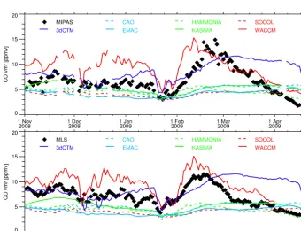
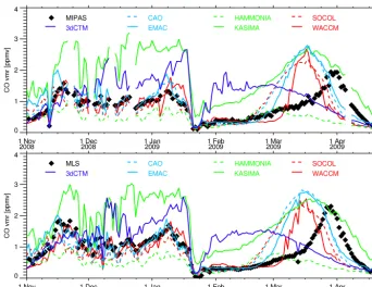
A more quantitative analysis is provided by Figs. 10 and 11, comparing the modelled CO evolutions at 0.02 and 0.5 hPa, respectively, to MIPAS-NOM and MLS observa-tions (note that FinROSE is not included here because of
[image:16.612.53.543.63.469.2]Figure 9.MIPAS-NOM and modeled temporal evolutions of CO at 4–0.02 hPa within 70–90◦N. White lines indicate the observed VMR levels of 0.3, 1, 3, and 10 ppmv.
✶ ✁✂ ✷✄ ✄☎
✶✆✝✞ ✷✄✄☎
✶✟✠ ✡ ✷✄✄☛
✶☞✝✌ ✷✄ ✄☛
✶✍ ✠✎ ✷✄✄☛
✶✏ ✑✎ ✷ ✄✄☛ ✄
✺ ✶✄ ✶✺ ✷✄
❈
✒
✓
✔
✕
✖
✗
✗
✔
✓
✘
✍ ▼ ✙✏ ✚
✸✛✜✢✍
✜✏ ✣ ❊✍✏✜
❍✏ ✍ ✍✣ ▼✏ ❑✏ ✚▼ ✍ ✏
✚✣✜✣ ❙ ❲✏✜✜✍
✤✥ ✦✧ ★✩ ✩✪
✤✫✬✭ ★✩✩✪
✤✮✯ ✰ ★✩✩✱
✤✲✬✳ ★✩ ✩✱
✤✴ ✯✵ ★✩✩✱
✤✹ ✻✵ ★ ✩✩✱ ✩
✼ ✤✩ ✤✼ ★✩
✽
✾
✿
❀
❁
❂
❃
❃
❀
✿
❄
✴ ❅ ❆
❇❉❋●✴
❋✹ ■ ❏✴✹❋
▲✹ ✴ ✴■ ✥◆✹ ❖✹ ❆◆ ✴ ✹
❆■❋■ ❅ P✹❋❋✴
[image:17.612.127.468.404.665.2]✶ ✁✂ ✷ ✄ ✄☎ ✶✆✝ ✞ ✷✄✄ ☎ ✶✟✠✡ ✷ ✄✄☛ ✶☞✝ ✌ ✷ ✄ ✄☛ ✶✍ ✠✎ ✷ ✄✄☛ ✶✏✑ ✎ ✷ ✄ ✄☛ ✄ ✶ ✷ ✸ ✹ ❈ ✒ ✓ ✔ ✕ ✖ ✗ ✗ ✔ ✓ ✘ ✍▼ ✙✏✚ ✸✛✜ ✢✍ ✜✏✣ ❊✍✏✜ ❍✏✍✍✣ ▼✏ ❑✏✚▼✍✏ ✚ ✣✜✣❙ ❲✏✜ ✜✍ ✤✥ ✦✧ ★ ✩ ✩✪ ✤✫✬ ✭ ★✩✩ ✪ ✤✮✯✰ ★ ✩✩✱ ✤✲✬ ✳ ★ ✩ ✩✱ ✤✴ ✯✵ ★ ✩✩✱ ✤✺✻ ✵ ★ ✩ ✩✱ ✩ ✤ ★ ✼ ✽ ✾ ✿ ❀ ❁ ❂ ❃ ❄ ❄ ❁ ❀ ❅ ✴❆ ❇ ✼❉❋ ●✴ ❋✺ ■ ❏✴✺❋ ▲✺✴✴ ■✥ ◆✺ ❖✺❇◆✴✺ ❇■❋■❆ P✺❋ ❋✴
Figure 11.MIPAS-NOM (top) and MLS/Aura (bottom) temporal evolutions of CO VMR in comparison with the model results within 70–90◦N at 0.5 hPa.
in slightly increased abundances during early winter. Fur-ther, minor differences in the late-winter abundances simu-lated by KASIMA and CAO on the one hand and EMAC and SOCOL on the other hand can be attributed to the use of different kinetic data in the chemistry schemes, primar-ily affecting OH involved in the CO loss reaction. The ob-served CO evolution at 0.02 hPa is qualitatively well cap-tured by WACCM, although the abundances during the pre-SSW phase of about 10 ppmv are overestimated by∼40 % compared to the observations and the ES-related peak oc-curs earlier than in the observations. HAMMONIA CO abun-dances are underestimated due to missing thermospheric CO production mechanisms (see previous section) and are very close to the CO amount simulated by the medium-top models (∼5 ppmv). 3dCTM simulates early-winter CO abundances that are roughly in agreement with the observations. ES-related CO enhancements in the post-SSW phase, however, are delayed and persist for a longer period than observed.
The observed CO evolution at 0.5 hPa is well reproduced by most medium-top models and WACCM in the pre-SSW phase. KASIMA and 3dCTM overestimate the CO abun-dances by a factor of ∼2.5 and ∼1.5, respectively, while HAMMONIA simulates about 50 % lower than observed CO abundances. The ES-related CO increases peak in most models too early (around mid-March) compared to the ob-served peak occurrence around 1 April, although the peak magnitude is reasonably well simulated (with exception of HAMMONIA). The CO peak in HAMMONIA occurs even
2 weeks earlier than in the other models. In 3dCTM, the CO tongue does not reach the 0.5 hPa level (see Fig. 9), likely because of the too-late formation of the elevated stratopause discussed in the previous section. The high CO abundances of this model in February, immediately after the SSW, seem to be caused by horizontal mixing, after a short period of lo-calized upwelling during the sudden warming.
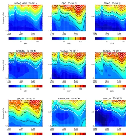
Figure 12.MIPAS-NOM and modelled temporal evolutions of NOxin the pre-SSW phase of the 2008/09 NH winter at 1–0.02 hPa within
70–90◦N. White lines indicate the observed VMR levels of 10, 20, 50, 70, 100, and 150 ppbv. White regions reflect missing or not meaningful data.
(see Fig. 18). Further, our 3dCTM results share some char-acteristics of the CMAM simulation without any GWD. In particular, both simulations exhibit a steady (though fluctu-ating) increase of CO until the SSW, a short recovery time after the warming, and the absence of an ES-related peak in March/April. This again highlights the importance of the proportion of the gravity wave spectrum not considered in the LIMA model – the subscale (≤500 km) waves for the mesospheric meridional wintertime circulation, in particular during the recovery phase of the elevated stratopause event as discussed in the previous section, but also for the “undis-turbed” pre-event period.
7.2 NOxin the early (pre-SSW) phase
In the following, the observed and modelled vertical struc-ture of NOxin the USM during mid-winter (pre-SSW phase)
is analysed in more detail to evaluate how well the models reproduce the EPP indirect effect in this region for unper-turbed conditions. Figure 12 compares the NOxevolution of
all models at 1–0.02 hPa with the MIPAS data. All models capture the observed early-winter NOxdescent characterized
by a quasi-continuous increase of NOxuntil the SSW-related
disruption in mid-January. The magnitude of the observed NOxenhancements is well reproduced by EMAC, FinROSE,