This is a repository copy of Temporal variations in supraglacial debris distribution on Baltoro Glacier, Karakoram between 2001 and 2012.
White Rose Research Online URL for this paper: http://eprints.whiterose.ac.uk/120443/
Version: Accepted Version
Article:
Gibson, M.J., Glasser, N.F., Quincey, D.J. et al. (3 more authors) (2017) Temporal
variations in supraglacial debris distribution on Baltoro Glacier, Karakoram between 2001 and 2012. Geomorphology, 295. pp. 572-585. ISSN 0169-555X
https://doi.org/10.1016/j.geomorph.2017.08.012
Article available under the terms of the CC-BY-NC-ND licence (https://creativecommons.org/licenses/by-nc-nd/4.0/).
eprints@whiterose.ac.uk https://eprints.whiterose.ac.uk/
Reuse
This article is distributed under the terms of the Creative Commons Attribution-NonCommercial-NoDerivs (CC BY-NC-ND) licence. This licence only allows you to download this work and share it with others as long as you credit the authors, but you can’t change the article in any way or use it commercially. More
information and the full terms of the licence here: https://creativecommons.org/licenses/
Takedown
If you consider content in White Rose Research Online to be in breach of UK law, please notify us by
Temporal variations in supraglacial debris distribution on
1
Baltoro Glacier, Karakoram between 2001 and 2012
2
Morgan J. Gibson1*, Neil F. Glasser1, Duncan J. Quincey2, Christoph Mayer3, Ann V.
3
Rowan4, Tristram D.L. Irvine-Fynn1,
4
5
1
Department of Geography and Earth Sciences, Aberystwyth University, Aberystwyth, UK
6
2School of Geography, University of Leeds, Leeds, UK
7
3
Commision for Geodesy and Glaciology, Bavarian Academy of Sciences and Humanities,
8
Munich, Germany.
9
4
Department of Geography, University of Sheffield, Sheffield, UK
10
11
12
*Corresponding author: mog2@aber.ac.uk
13
14
15
16
17
18
19
20
21
22
23
Abstract 25
Distribution of supraglacial debris in a glacier system varies spatially and temporally due to
26
differing rates of debris input, transport and deposition. Supraglacial debris distribution
27
governs the thickness of a supraglacial debris layer, an important control on the amount of
28
ablation that occurs under such a debris layer. Characterising supraglacial debris layer
29
thickness on a glacier is therefore key to calculating ablation across a glacier surface. The
30
spatial pattern of debris thickness on Baltoro Glacier has previously been calculated for one
31
discrete point in time (2004) using satellite thermal data and an empirically based
32
relationship between supraglacial debris layer thickness and debris surface temperature
33
identified in the field. Here, the same empirically based relationship was applied to two
34
further datasets (2001, 2012) to calculate debris layer thickness across Baltoro Glacier for
35
three discrete points over an 11-year period (2001, 2004, 2012). Surface velocity and
36
sediment flux were also calculated, as well as debris thickness change between periods.
37
Using these outputs, alongside geomorphological maps of Baltoro Glacier produced for
38
2001, 2004 and 2012, spatiotemporal changes in debris distribution for a sub-decadal
39
timescale were investigated. Sediment flux remained constant throughout the 11-year
40
period. The greatest changes in debris thickness occurred along medial moraines, the
41
locations of mass movement deposition and areas of interaction between tributary glaciers
42
and the main glacier tongue. The study confirms the occurrence of spatiotemporal changes
43
in supraglacial debris layer thickness on sub-decadal timescales, independent of variation
44
in surface velocity. Instead, variation in rates of debris distribution are primarily attributed to
45
frequency and magnitude of mass movement events over decadal timescales, with climate,
46
regional uplift and erosion rates expected to control debris inputs over centurial to millennial
47
timescales. Inclusion of such spatiotemporal variations in debris thickness in distributed
48
surface energy balance models would increase the accuracy of calculated ablation, leading
to a more accurate simulation of glacier mass balance through time, and greater precision
50
in quantification of the response of debris-covered glaciers to climatic change.
51
52
Keywords: Karakoram, debris-covered glaciers, supraglacial debris, Baltoro Glacier
53
54
55
1. Introduction
56
Debris-covered glaciers are commonly found in tectonically-active mountain ranges
57
including the Andes, the Southern Alps of New Zealand and the Himalaya-Karakoram
58
(Kirkbride, 1999; Scherler et al., 2011). High rates of rock uplift and erosion and steep
59
hillslopes in these regions cause large volumes of rock debris to be incorporated into
60
glacier systems, and ultimately form supraglacial debris layers of varying thicknesses and
61
extents (Anderson and Anderson, 2016; Shroder et al., 2000). The presence of a
62
supraglacial debris layer affects ablation of the underlying ice (Evatt et al., 2015; …strem,
63
1959), because the debris acts as a thermal barrier between ice and atmosphere, ultimately
64
resulting in a non-linear response of debris-covered glaciers to climatic change (Benn et al.,
65
2012; Scherler et al., 2011). Glaciers in the Himalaya-Karakoram supply water to some of
66
the largest rivers in the world, including the Indus, Brahmaputra and Ganges (Bolch et al.,
67
2012). Consequently, the response of glaciers in the Himalaya-Karakoram to recent and
68
current climatic change will affect the lives of the 1.4 billion people in central Asia who rely
69
on these rivers as their primary water resource (Immerzeel et al., 2010).
70
71
Given that the proportion of debris-covered glacier ice area in the Himalaya-Karakoram
72
region is increasing (Deline, 2005; Mihalcea et al., 2006), gaining a full understanding of the
73
influence of debris layers on melt-rates is becoming increasingly pertinent. Typically,
supraglacial debris is initially entrained into lateral and medial moraines in the upper
75
reaches of the glacier. As moraines coalesce with increasing distance from their source the
76
debris layer becomes more spatially extensive (Anderson, 2000; Kirkbride and Deline,
77
2013). The thickness of the supraglacial debris layer increases down-glacier and reaches
78
its maximum near the glacier terminus (Anderson, 2000). In areas where supraglacial
79
debris cover extends across the entire glacier surface spatially variable debris distribution
80
results in differential melting and forms an undulating glacier surface topography (Hambrey
81
et al., 2008; Kirkbride and Deline, 2013). Supraglacial debris thickness varies in space and
82
time as a result of differing spatial extents and temporal rates of debris input, transport and
83
exhumation (Rowan et al., 2015). Ablation rates of debris-covered glaciers are therefore
84
also spatially and temporally variable (Benn et al., 2012; Rounce and McKinney, 2014).
85
Studies that consider the response of debris-covered glaciers to climatic change currently
86
do not account for this variability (e.g. Bolch et al., 2012; Scherler et al., 2011; Shea et al.,
87
2015), which increases the uncertainty in estimations of glacier ablation rates, and thus the
88
subsequent predictions of the response of debris-covered glaciers to climatic change.
89
90
The impact of supraglacial debris layers on melt rates is well established (e.g. …strem,
91
1959); thin debris layers (typically <0.05 m thick, depending on local conditions) enhance
92
ablation by increasing albedo of the glacier surface, while thicker debris layer attenuate
93
melt by insulation of the underlying ice (Mihalcea et al., 2008b; Nicholson and Benn, 2006;
94
…strem, 1959). Ablation is maximized at an effective debris thickness (commonly 0.01Ð0.02
95
m), while the critical thickness of debris (ranging from 0.02 to 0.1 m), where ablation under
96
debris-covered ice is equal to that of debris-free ice, is defined by debris properties such as
97
lithology, porosity, grain size distribution, moisture content and surface roughness of the
98
debris layer (Brock et al., 2010; Kayastha et al., 2000). The amount of ablation under a
debris layer is also affected by external factors such as the transfer rate of precipitation
100
through a debris layer, glacier surface topography, and the occurrence of suprafluvial
101
networks and associated sediment transport processes, all of which are spatially and
102
temporally variable (Seong et al., 2009).
103
104
Measuring the thickness distribution of a supraglacial debris layer is challenging in the field
105
due to high spatial variability in debris layer thickness over short distances, difficulties in
106
excavating such debris layers (Mayer et al., 2006), and an inability to capture such
107
variability with point data. Early work put forward the idea of using thermal characteristics of
108
supraglacial debris to define its extent from satellite data (Ranzi et al., 2004). Subsequent
109
projects developed the use of such thermal satellite data to estimate debris thickness for
110
entire glacier surfaces: a glacier-specific relationship between surface temperature and
111
debris thickness is identified using field point data, which is subsequently applied to
112
satellite-derived thermal data of the entire glacier area (e.g. Foster et al., 2012; Rounce and
113
McKinney, 2014; Mihalcea et al., 2008a; Mihalcea et al., 2008b; Soncini et al., 2016). These
114
maps have advanced understanding of spatial variability in debris thickness, but usually
115
only represent a discrete point in time. Minora et al. (2015) enabled the observation of
116
temporal changes in debris thickness by producing a second debris thickness map of
117
Baltoro Glacier for 2011, in addition to the one produced by Mihalcea et al. (2008b) for
118
2004. However, Minora et al. (2015) did not explore the extent of debris thickness change
119
between the two periods. Consequently, little is known about the rate at which changes in
120
supraglacial debris layer thickness occur, an essential parameter for understanding the
121
transport of debris by ice flow and the localised redistribution of the debris over a glacier
122
surface, which can be used to validate precise numerical modelling of the dynamics of
debris-covered glaciers through time (e.g. Anderson and Anderson, 2016; Rowan et al.,
124
2015).
125
126
In this study, we investigated supraglacial debris on Baltoro Glacier in Pakistan to: (1)
127
identify the spatio-temporal variation in supraglacial debris distribution on Baltoro Glacier
128
between 2001 and 2012; (2) consider some of the processes that control these variations
129
in debris distribution using surface velocity and geomorphological mapping; and (3)
130
calculate annual rates of debris thickness change and sediment flux on Baltoro Glacier
131
using debris thickness and surface velocity maps. We subsequently comment on how such
132
calculations can be used in numerical models for glaciers.
133
134
2. Study area
135
Baltoro Glacier is located in the eastern Karakoram mountain range in northern Pakistan
136
(35¡35Õ N, 76¡04Õ E; Figure 1). The glacier is 62 km long and flows from near the peak of K2
137
(8611 m a.s.l.) to an altitude of 3410 m a.s.l. (Mayer et al., 2006; Mihalcea et al., 2008b)
138
(Figure 1a). A number of tributary glaciers feed Baltoro Glacier (Figure 1b), including
139
Baltoro South and Godwin-Austen Glaciers, which converge to form the main Baltoro
140
Glacier tongue at Concordia (4600 m). The surface velocity of Baltoro Glacier varies along
141
its length, with a maximum surface velocity of ~200 m a-1 below Concordia, decreasing to
142
less than 15 m a-1 close to the glacier terminus (Copland et al., 2009; Quincey et al., 2009).
143
Surface velocity was observed to increase in 2005 (Quincey et al., 2009), attributed to an
144
abundance of meltwater being routed to the bed and thus reducing basal friction.
145
146
The ablation area of Baltoro Glacier is almost entirely debris covered. Up-glacier of
147
Concordia, supraglacial debris is predominantly entrained into medial and lateral moraines
that punctuate the clean ice surface, with a lesser contribution of mass movement deposits
149
along the glacier margins (Mihalcea et al., 2006). The debris layer is thinnest (0.01Ð0.15 m)
150
in the upper ablation area of the glacier and exceeds 1 m at the glacier terminus (Mihalcea
151
et al., 2008b). Supraglacial debris units have differing lithologies across the debris-covered
152
glacier surface, which include granite, schist, gneiss and metasediments (Gibson et al.,
153
2016).
154
155
Figure 1. (a) Baltoro Glacier in a regional context; (b) the tributary glaciers of Baltoro
156
Glacier (numbered) and (c) Baltoro Glacier and its tributary glaciers.
157
158
3. Methods 159
3.1. Debris thickness
[image:8.595.123.463.257.573.2]Advanced Spaceborne Thermal Emission and Reflection Radiometer (ASTER) thermal
161
data were used to derive debris thickness on Baltoro Glacier for three discrete periods in
162
time; 2001, 2004 and 2012 (Table 1). The 2004 dataset was the same as that used by
163
Mihalcea et al. (2008b) for production of their 2004 debris thickness map of Baltoro Glacier.
164
The 2001 and 2012 data sets were chosen due to their low cloud cover, resulting in minimal
165
glacier area being obscured. ASTER imagery was downloaded from NASAÕs Earth
166
Observing System Data and Information System (http://reverb.echo.nasa.gov) as a Level 2
167
surface kinetic temperature product (AST_08). Level 2 surface kinetic temperature data are
168
comprised of mean surface temperature calculated from thermal bands 11Ð15. Prior to
169
delivery, surface kinetic temperature data are atmospherically corrected and converted from
170
top-of-atmosphere temperature to surface temperature. ASTER thermal data have a spatial
171
resolution of 90 m and temperature resolution of 0.5 K (Abrams and Ramachandran, 2002).
172
The 2001 and 2012 ASTER datasets were both acquired in August within 15 days of the
173
original 2004 dataset, therefore allowing for seasonal variation in debris surface to be
174
minimised as much as possible when comparing subsequent outputs. All outputs were
co-175
registered to within a pixel through manual placement of 50 tie points between each image
176
pair prior to calculation of debris thickness, to avoid any spatial mismatch between the input
177
layers. The images were also orthorectified using the rigourous orthorectification tool in
178
ENVI (v. 5.0) and the ASTER digital elevation model (2011) at 30 m resolution, which
179
corrects for the effect of sensor tilt and terrain, and produced an RMSE of 5.82 m. Debris
180
thickness was derived using the methods detailed in Mihalcea et al. (2008b). Equation 1
181
was applied to the same satellite image used by Mihalcea et al. (2008b) to yield debris
182
thickness for 2004:
183
!
184
! ! !!!! DT!exp!!!!0192!!!!–58!7174! (1)
186
Where DT is debris thickness and !!! is surface temperature. The same method was then 187
applied to the 2001 and 2012 ASTER data for Baltoro Glacier to yield a time-series of
188
debris thickness maps.
189
190
191
192
Table 1. Satellite ID, acquisition date and time and mean debris thickness for ASTER
193
datasets used for calculating debris thickness (grey boxes) and surface velocity.
194
195
Satellite data I.D. Acquisition date
and time
Mean debris thickness (m)
AST_08_00308292001060003 _20140108123858_15605
29/08/2001 06:00
0.14
AST_08_00310032002055404 _20151109052624_814
03/09/2002 05:54
AST_08_00308142004054614 _20151109052424_30691
14/08/2004 05:46
0.21
AST_08_00310122008054700 _20151109052644_888
12/09/2008 05:47
AST_08_00305052011055248 _20151109052354_30515
05/09/2011 05:52
AST_08_00308202012054630 _20151109052624_816
20/08/2012 05:46
0.45
196
197
198
Debris thickness change was calculated between the 2001Ð2004 and 2004Ð2012 debris
199
thickness maps. In both cases the earlier debris thickness map was subtracted from the
later map to yield debris thickness change for each time period, and then divided by the
201
number of years between the two maps to calculate mean annual debris thickness change.
202
203
Uncertainty in the calculated debris thickness was estimated for the 2012 debris thickness
204
map using field debris thickness measurements collected in 2013 (Figure 1c). Mean annual
205
debris thickness change calculated from the 2004Ð2012 debris change map (0.03 m a-1)
206
was added to the 2012 debris thickness to provide projected debris thickness for 2013. To
207
calculate uncertainty the 17 field-derived debris thickness point measurements were
208
compared to debris thicknesses from the corresponding pixels in the projected 2013 debris
209
thickness map (Table 2). Mean variation in debris thickness between 2013 field data and
210
projected 2013 debris thickness was 0.090 m, 0.064 m above the uncertainty calculated for
211
the 2004 debris thickness map by Mihalcea et al. (2008b) of 0.026 m. Consequently, in this
212
study uncertainties for the debris thickness maps were estimated as 0.026 m for 2004 and
213
0.090 m for 2012. Uncertainty for the 2001 debris thickness map could not be calculated
214
due to a lack of field data collected prior to 2004. Additional parameters such as moisture
215
content in and thermal inertia of the debris layer may have also affected estimations of
216
supraglcial debris layer thickness calculated using Mihalcea et al.Õs (2008b) method, but the
217
low uncertainty values calculated here suggest they have minimal effect on the outputs
218
presented.
219
220
Due to a lack of field data in debris layers with a thickness greater than 0.5 m uncertainty
221
values calculated here are only applicable for debris layers with a thickness ≤ 0.5 m. Above
222
0.5 m debris surface temperature is considered independent of debris layer thickness
223
(Nicholson and Benn, 2006). Consequently, analysis of these debris thickness maps is
focused on areas of the glacier where debris thickness is ≤0.5 m, and analysis of debris
225
thickness maps are presented alongside geomorphological evidence for justification.
226
227
228
Table 2. Comparison of field point debris thickness data to corresponding pixel value (plus
229
one yearÕs annual rate of debris thickness change), used to calculate error between the
230
2012 satellite-derived debris thickness map and field data.
231
Point I.D. 2013 in situ
debris thickness (m)
2013 satellite-derived debris
thickness (m)
Difference (m)
1 0.02 0.01 0.01
2 0.00 0.07 0.07
3 0.09 0.23 0.14
4 0.13 0.15 0.02
5 0.01 0.04 0.03
6 0.06 0.03 0.03
7 0.04 0.02 0.02
8 0.05 0.14 0.09
9 0.075 0.02 0.05
10 0.04 0.23 0.19
11 0.12 0.39 0.27
12 0.07 0.18 0.11
13 0.17 0.06 0.11
14 0.04 0.14 0.10
15 0.26 0.28 0.02
16 0.1 0.01 0.09
17 0.43 1.16 0.73
Mean difference:
Standard deviation:
0.09
0.50
[image:12.595.95.500.266.732.2]233
3.2. Glacier dynamics and surface morphology
234
3.2.1. Surface velocity analysis
235
Glacier surface velocity analysis was undertaken in ENVI (v.5.0) using the feature tracking
236
plugin tool Cosi-Corr (Leprince et al., 2007). Cosi-Corr is a Fourier-based image correlation
237
tool that offers sub-pixel accuracy for the measurement of horizontal offsets (Scherler et al.,
238
2011). ASTER Band 3N data (Visible Near Infrared, Wavelength: 0.760Ð0.860 nm,
239
resolution: 15 m) were used for feature tracking. Image pairs used were acquired in 2001
240
and 2002, 2003 and 2004, and 2011 and 2012 (Table 1), and were co-registered to
sub-241
pixel level prior to calculation of surface displacement. All results were converted to annual
242
displacements for comparison. A variable window size between 128 and 64 pixels and a
243
step size of one pixel was used for all velocity outputs, and absolute surface velocity
244
derived from north-south and east-west velocity fields. North-south and east-west velocity
245
fields were used for identification of direction of maximum surface velocity in the calculation
246
of sediment flux. Velocity outputs were masked using a velocity threshold of 200 m a-1 to
247
exclude erroneous results in ENVI (v. 5.0), and clipped to the extent of a
manually-248
improved Baltoro Glacier outline based on the Randolph Glacier Inventory outline (v. 5.0;
249
Arendt et al., 2012), used in Gibson et al. (2016) in ArcMap (v.10.1). Pixels with erroneous
250
surface velocity values (less than zero or above 200 m a-1, or pixels with substantially
251
different velocity values to the surrounding pixels) were masked from the final surface
252
velocity maps.
253
254
3.2.2. Geomorphological mapping
255
Geomorphological features on the surface of Baltoro Glacier, including debris units, mass
256
movement deposits, supraglacial water bodies and crevasses, were mapped using the
optical bands (15 m resolution) of the same three time-separated and orthorectified ASTER
258
data sets used for deriving debris thickness (August 2001, 2004 and 2012). ASTER images
259
were orthorectified using the ASTER digital elevation model at 30 m resolution. Additionally,
260
a Landsat 7 Enhanced Thematic Mapper (ETM+) image, acquired in August 2001 at 30 m
261
resolution, was used to map regions of the glacier covered in cloud in the ASTER August
262
2001 imagery. All satellite datasets used were co-registered prior to mapping. Features
263
were mapped using a false-colour composite (Bands 3N, 2, 1) and were manually digitised
264
in ESRI ArcGIS (v. 10.1). Debris units were classified using their differing spectral
265
reflectance profiles (Figure 2; Lillesand et al., 2014). The debris units were then traced
up-266
glacier to their source area and lithology identified using the regional geological map
267
produced by Searle et al. (2010). Spectra from 200 pixels were then compared to spectra
268
from the USGS spectral library in ENVI to confirm correct classification. 91% of sampled
269
pixels were correctly classified based on these independent data. Mass movement
270
deposits were identified by the presence of two features: a scar, identified as an elongate
271
feature on the valley side which differed in colour to the surrounding valley wall, suggesting
272
erosion and loss of vegetation had occurred, and an associated lobate debris fan deposit
273
on or near the glacier surface. A Normal Difference Water Index (NDWI) was used to
274
identify pixels containing supraglacial water, calculated from ASTER bands 3 (Near
275
Infrared; NIR) and 4 (Shortwave Infrared: SWIR) after (Gao, 1996):
276
277
NDWI = (NIR (Band 3) Ð SWIR (Band 4))/ (NIR (Band 3) + SWIR (Band 4)) (2)
278
279
The classification of water was verified through manual comparison of 100 randomly
280
selected features classified as water in the 2011 ASTER imagery with high resolution (2.5
281
m) Quickbird imagery from 2011 for the same locations. All 100 features were identified as
water in both images, and so were assumed to be correctly classified. The area of debris
283
units and supraglacial water bodies were derived using the geometry calculator in ArcGIS
284
(v.10.1).
285
286
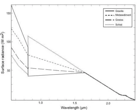
Figure 2: Spectral reflectance profiles for the different lithology types identified on Baltoro
287
Glacier. 288
289
3.3. Sediment flux
290
Supraglacial sediment flux across the glacier surface was calculated using derived debris
291
thickness and surface velocity data, following the method developed by Heimsath and
292
McGlynn (2008) to determine headwall retreat rate on MilarepaÕs Glacier in Nepal.
293
Heimsath and McGlynn (2008) measured debris thickness and surface velocity along one
294
transect near the glacier headwall, then calculated cross-sectional area of the debris using
295
the debris thickness transect, and multiplied the cross-sectional area by surface velocity,
296
calculating one-dimensional sediment flux. Here, we calculated supraglacial sediment flux
297
for each pixel by multiplying debris thickness by the pixel width at right angles to the
298
direction of maximum surface velocity to give supraglacial debris layer cross-sectional area,
[image:15.595.181.414.186.373.2]and then multiplied cross-sectional area by surface velocity for the same pixel. As surface
300
velocity and supraglacial debris thickness were used to calculate sediment flux these
301
results only represent debris transported supraglacially. The resulting sediment flux maps
302
were normalized to annual datasets to obtain comparable sediment flux values, and were
303
masked using the same masks applied to the surface velocity and debris thickness maps to
304
exclude pixels with erroneous results and cloud cover.
305
306
4. Results 307
4.1. Debris thickness
308
A similar pattern of debris thickness distribution was present in 2001, 2004 and 2012
309
(Figure 3). In the upper section of the glacier above and around Concordia, debris was
310
distributed in alternating bands of thicker debris (around 0.2Ð0.3 m thick) and thin,
sparsely-311
distributed or non-existent debris layers (≤ 0.02 m), in a longitudinal pattern parallel to ice
312
flow. Thicker bands of debris originated from the glacier margin, primarily at confluences
313
between tributary glaciers and the main glacier tongue, which were interpreted to be medial
314
moraines. In the glacier mid-section, debris coverage became increasingly spatially
315
extensive with decreasing distance from the glacier tongue, and a general thickening of
316
debris towards the glacier terminus occurred. No build up of debris, such as that expected
317
where a terminal moraine is present, was observed at the glacier terminus from satellite
318
data, confirming the absence of such a feature previously observed in the field by Desio
319
(1954). Debris covered the entire glacier surface in the lower section of the glacier and was
320
predominantly > 0.5 m thick.
322
Figure 3: Debris thickness maps of Baltoro Glacier for: (a) August 2001; (b) August 2004;
323
(c) August 2012. 324
325
The broad, glacier-wide pattern of debris distribution displayed minimal change between
326
2001 and 2012, suggesting that a pattern of debris input and transport was already
327
established across the glacier and persisted over the study period. However, the thickness
328
of the debris layers across the glacier varied over the 11-year study period. Cloud cover in
329
2001 restricted comparison between 2001 and 2004 in the glacierÕs lower section, but
330
Debris thickness (m)
Cloud cover No data
0.0 - 0.03 0.031 - 0.06 0.061 - 0.10 0.101 - 0.15 0.151 - 0.2 0.201 - 0.3 0.301 - 0.4 0.401 - 0.5 0.501 - 1.0 1.001 - 3.0
0 10 km
N
a) August 2001
b) August 2004
c) August 2012
2 1
10 9
8
7
6
5 4
3 11
12
13 14
[image:17.595.146.465.100.489.2]thickening of the medial moraines in the glacier upper-section of the order of around 0.1m
331
was seen during this 3-year time period. A general trend of increasing debris thickness in
332
the glacier mid-section was seen between 2001 and 2012, with a mean debris layer
333
thickness in the glacier mid-section of ~0.28 m in 2001, ~0.34 m in 2004 and ~0.41 m in
334
2012. Debris thickness was most variable in the glacier lower section between 2004 and
335
2012, with a mean debris layer thickness of ~0.71 m in 2004 and ~1.5 m in 2012, and an
336
apparent thickening of debris at the terminus, although further field data would be needed
337
to confirm these mean debris thicknesses due to the independence of debris surface
338
temperature with debris layer thickness above 0.5 m. Increasing debris thickness in the
339
lower and mid sections suggests a progressive backing up of debris through time causing
340
the area of thickest debris to increase up-glacier from the terminus.
341
342
In 2004 a sharp boundary between debris layer thicknesses was observed running
343
longitudinally from the glacier terminus to the location at which Trango Glacier (Tributary
344
Glacier 9) joins the main glacier tongue (Figures 1b; 3). South of the boundary debris
345
thickness was above 0.5 m thick, whilst north of the boundary debris layer thickness was
346
less than 0.5 m thick. The debris thickness boundary correlates with the boundary between
347
a granite debris unit originating on Trango Glacier and gneiss debris units of the main
348
glacier tongue, presumed to also be the boundary between the main glacier flow units and
349
Trango Glacier flow unit.
350
351
4.2. Glacier surface velocity
352
A general trend of highest velocity at Concordia, where Baltoro South and Godwin-Austen
353
Glacier converge, and subsequently decreasing surface velocity down-glacier of Concordia
354
towards the terminus was observed at all time periods, with very low (less than 20 m a-1) to
no glacier flow near the terminus (Figure 4). Variations in surface velocity occurred between
356
2001 and 2012, with an average decrease in surface velocity of around 50 m a-1 along the
357
longitudinal profile of the glacier (Figure 4a) between 2001 and 2004, followed by an
358
increase on the same order of magnitude between 2004 and 2012 (Figure 4d). Higher
359
surface velocities were observed at Concordia where the Godwin-Austen and Baltoro South
360
Glaciers join, and subtle velocity increases at some but not all tributary glacier confluences
361
were also noted (e.g. Yermanendu and Mandu glaciers; Tributary glaciers 4 and 5,
362
respectively). In 2012 glacier surface velocity was lowest (~0Ð20 m a-1) in the northwest
363
region of the terminus, a triangular shaped area which extended from the glacier terminus
364
and pinched out at around 5 km up-glacier of the terminus and downstream of Trango
365
Glacier. However, in 2004 no such pattern was evident and a patchy distribution of velocity
366
between 0 and 50 m a-1 across the glacier width for around 10 km up-glacier of the
367
terminus occurred.
369
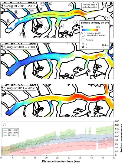
Figure 4: Surface velocity maps in m a-1 for Baltoro Glacier for: (a) 2001, (b) 2004 and (c)
370
2012, and (d) surface velocity profiles along the centre line of the main glacier tongue with
371
uncertainty values of each velocity line displayed with shaded regions.
372
0
Surface velocity (m a-1)
0 200
No data Flowline used in velocity profiles
0 10 km
N a) August 2001 – 2002
b) August 2004 – 2003
c) August 2011 – 2012
0 20 40 60 80 100 120 140 160 180
0 5 10 15 20 25 30 35 40 45 50
Distance from terminus (km)
Su
rfa
c
e
v
e
lo
c
ity
(m
a
-1) d)
2001–2002 2003–2004 2011–2012
2 1 10
9
8 6
5 4
3
11
12 13
14
[image:20.595.106.509.96.635.2]4.3. Geomorphological features 373
Supraglacial debris lithology was identified through comparison of ASTER pixel spectra with
374
spectra of lithologies from the USGS spectral library and with reference to the geology map
375
produced by Searle et al. (2010). The supraglacial debris on Baltoro Glacier was dominated
376
by gneiss (~51Ð53 % of the debris-covered glacier area), whilst ~47Ð49 % was composed
377
of granite (~27 %), schist (~12 %) and a small proportion of metasediment (~6 %) (Figure
378
5, Table 3). Across the main glacier tongue, negligible change in debris unit boundaries
379
occurred between 2001 and 2012 and change in percentage cover of debris units was
380
attributed to errors produced by manual digitisations (Gibson et al., 2016; Table 3).
381
However, small scale variations in debris distribution did occur on tributary glaciers between
382
2001 and 2012, which have been attributed to these glaciers being in various periods of
383
instability, possibly related to surge phases,, and input of debris material from surrounding
384
valley walls through rock- and snow avalanches (Gibson et al., 2016). For example,
385
patches of thicker debris on Mandu Glacier (Tributary Glacier 5) can be tracked
down-386
glacier between 2001 and 2012 in geomorphological maps (Figure 6d) and debris thickness
387
maps (Figure 6e), with debris initially deposited on the glacier by a mass movement event
388
and then transported as a bulk volume.
389
390
391
392
394
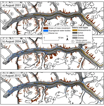
Figure 5: The surface geomorphology of Baltoro Glacier in (a) August 2001, (b) August
395
2004 and (c) August 2012.
396
397
398
399
400
401
Areas of mass movement
Supraglacial water bodies Metasediments Schist Granite Gneiss
Debris rock types
Glacier ice
10 km
0 N
a) August 2001
b) August 2004
c) August 2012
2 1
9
8
6
5
4 3
11
7
10
13 14
12
Tributary glacier identification number
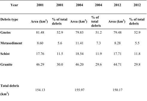
[image:22.595.88.515.74.512.2]Table 3. Total area of each debris unit type, based on lithology, for 2001, 2004 and 2012,
402
and the percentage of each debris type as a proportion of the total debris cover for Baltoro
403
Glacier and its tributary glaciers (Gibson et al., 2016). Variability in total debris area is
404
attributed uncertainty produced by manual digitisation.
405
406
Year 2001 2001 2004 2004 2012 2012
Debris type
Area (km2) % of total
debris Area (km
2
)
% of total debris
Area (km2) % of total debris
Gneiss 81.48 52.9 79.83 51.2 79.48 52.9
Metasediment 8.60 5.6 11.41 7.3 8.28 5.5
Schist 17.76 11.5 18.54 11.9 17.71 11.8
Granite 46.29 30.0 46.20 29.6 44.71 29.8
Total debris
(km2)
154.13 155.97 150.17
407
408
409
410
411
412
413
[image:23.595.58.549.210.547.2]Figure 6: Comparison of: (a) geomorphology, (b) debris thickness and, (c) debris thickness
415
change at the terminus of Baltoro Glacier, showing a distinct boundary between debris
416
thickness values and debris units of different lithologies; (d) geomorphology, with previous
417
positions on areas of supraglacial debris from 2001 (red) and 2004 (green) displayed, (e)
418
debris thickness and (f) debris thickness change on Mandu Glacier (Tributary Glacier 5)
419
showing the down-glacier movement of debris pockets through time; (g) geomorphology
420
and (h) debris thickness of the confluence area between Godwin-Austen Glacier and
421
Baltoro South Glacier in 2012, showing an area of thick debris up-glacier of where the
422
tributary glaciers join and change direction to form the main glacier tongue.
423
a) Geomorphology 2012 b) Debris thickness 2012 c) Debris thickness change 2004 – 2012
0 2 km
d) Geomorphology e) Debris thickness 2004 f) Debris thickness change 2004 - 2012
0 1 km
Areas of mass movement Supraglacial water bodies
Metasediments Schist Granite Gneiss Glacier ice <-0.4 -0.39– -0.3 -0.29– -0.2 -0.19– -0.1 -0.09– -0.05 -0.05–0.1 0–0.05 0.05–0.1 0.11–0.2 0.21–0.3
Debris thickness change (m a-1)
0.0 - 0.03 0.031 - 0.05 0.061 - 0.1 0.101 - 0.15 0.101 - 0.2 0.201 - 0.3 0.301 - 0.4 0.401 - 0.5 0.501 - 1.0 1.001 - 3.0
Geomorphology Debris thickness (m)
0.31–0.4 >0.4 g) Geomorphology 2012 h) Debris thickness 2012
0 2 km
9 8 9 8 9 8
5 5 5
2 2
1 1
Tributary glacier identification number 1
Location of 2001 debris Location of 2004 debris
Supraglacial water bodies occurred most frequently in the lower to lower-mid-sections of
424
the glacier between 2001 and 2012, and in areas of relatively thick debris, such as east of
425
the confluence between Goodwin-Austen and Baltoro South Glaciers (Figure 6g and 6h).
426
However, at all time points an absence of supraglacial water bodies was present in the
427
gneiss debris unit at the terminus of the main glacier tongue and around the terminus of
428
Tributary Glacier 8 (unnamed). The number of supraglacial water bodies increased by 336
429
over the study period, from 234 in 2001 to 570 in 2012 (Table 4). Total area of supraglacial
430
water bodies increased by almost 400 % during the same period. Temporally, the greatest
431
change in water body number and area occurred between 2001 and 2004, whilst spatially
432
the greatest increase in water body number occurred in the lower mid-section and east of
433
Concordia at up-glacier margin of the confluence between Godwin-Austen and Baltoro
434
South Glacier.
435
[image:25.595.60.525.486.597.2]436
Table 4. Supraglacial water area and number on Baltoro Glacier in 2001, 2004 and 2012
437
(Gibson et al., 2016).
438
2001 2004 2012
Number of water bodies 234 404 570
Area (km2) 0.66 1.79 2.04
439
440
4.4. Annual debris thickness change
441
Mean annual debris thickness change (Figure 7) showed areas of debris thickness increase
442
predominantly occurred in the lower section of the glacier and along medial moraines, and
443
were of the order of 0.05 to 0.3 m a-1, greater than uncertainty values for debris thickness
maps. In areas of decreasing debris thickness a reduction in thickness of the order of 0.05Ð
445
0.09 m a-1 was observed, with most change occurring between 2001 and 2004, although
446
these areas of decrease were lower than the uncertainty values associated with the debris
447
thickness maps. Such areas of decreasing debris thickness occurred on the northern
448
margin of the main glacier tongue and parallel to debris layer thickening of medial
449
moraines. Debris thickening occurred at a similar rate and pattern in the lower section of the
450
glacier between the two periods, with the greatest increase along the boundary between the
451
main glacier tongue and Trango Glacier (Section 4.1). During both periods, increase in
452
debris thickness was primarily along the moraine crests in the mid-section of the glacier,
453
with more extensive increases between 2001 and 2004, extending to the glacier
upper-454
section. Debris thickness change on tributary glaciers was of the order of ±0.05 m a-1, with
455
specific areas of debris change apparent, including deposits on Mandu Glacier, considered
456
to have been derived from mass movement events which moved down-glacier through
457
time, revealed through a loss of thickness in their previous position and an increasing
458
debris thickness in the current position (Figure 6f).
460
Figure 7: Annual debris thickness change, calculated by subtracting the earlier debris
461
thickness map from the later, and then divided by the number of years between the two
462
maps, for (a) 2001 Ð 2004 and (b) 2004 Ð 2012.
463
464
4.5. Annual sediment flux
465
Supraglacial sediment flux (Figure 8) showed a similar spatial distribution for all points in
466
time, with the highest sediment flux (between 11000 and 12000 m3 a-1) in the lower section
467
of the glacier and along the northern glacier margin in the glacier mid-section. Areas of
468
higher sediment flux (>9000 m3 a-1) were also found at the confluence of tributary glaciers
469
and the main glacier tongue, such as east of Concordia (2003-2004), Yermanendu Glacier
470
(Tributary Glacier 4; 2001-2002) and Tributary Glacier 6 (unnamed; 2001-2002,
2003-471
b) 2004 - 2012 a) 2001 - 2004
(m a-1)
0 10 Km
<-0.4 -0.399– -0.30 -0.299– -0.20 -0.199– -0.10 -0.099– -0.05 -0.049– 0.001 0 – 0.050 0.051– 0.100 0.101– 0.200 0.201– 0.300
0.301– 0.4 > 0.4
N
Debris thickness change (m a-1) 2 1
9
8
6
5 4
3
11
7
10
13
14 12
Tributary glacier identification number 1
[image:27.595.108.494.82.435.2]2004). For a large proportion of the mid- and upper sections of the glacier, sediment flux
472
was generally less than 1000 m3 a-1, with some areas of relatively higher sediment flux
473
along moraine features (4000Ð6000 m3 a-1).
474
475
A general pattern of increasing sediment flux was seen between 2001Ð2002 and 2011Ð
476
2012 along medial moraines in the lower section of the glacier, with an increase in sediment
477
flux on the order of between 5000Ð6000 m3 a-1 between 2001 and 2002 to 6000Ð8000 m3 a
-478
1
between 2001 and 2012. In the upper-mid and upper-sections of the glacier these medial
479
moraines had a constant sediment flux of around 6000 m3 a-1. Although the sediment flux
480
maps do not extend to the initiation point of many of the medial moraines where debris is
481
introduced into the upper glacier system, consistency in sediment flux along moraine
482
features suggest input from valley wall erosion and entrainment was stable over the
sub-483
decadal period. In the 2001Ð2002 and 2003Ð2004 sediment flux maps pockets of sediment
484
flux less than 1000 m3 a-1 in the lower section of the glacier corresponded to the location of
485
supraglacial water bodies.
Figure 8: Sediment flux; debris cross-sectional area for each pixel multiplied by surface
487
velocity, for (a) 2001Ð2002, (b) 2003Ð2004 and (c) 2011Ð2012.
488
489
490
5. Discussion 491
5.1. Spatiotemporal change in supraglacial debris distribution
492
A debris distribution common to the majority of debris-covered glaciers is evident on the
493
surface of Baltoro Glacier throughout the study period, with the thickest debris occurring
494
near the terminus and along moraine crests, and an increasingly thick debris layer towards
495
0 12000
Sediment flux
6000 (m3 a-1)
No data
N0 10 km
a) August 2001
b) August 2004
c) August 2012
2 1
9
8
6
5 4
3
11
7
10
13 14
12
[image:29.595.118.496.81.503.2]the terminus (e.g. Figure 9; Fushimi et al., 1980; Kirkbride and Warren, 1999; Mihalcea et
496
al., 2006b; Zhang et al., 2011). A progressive increase in the area covered by debris
497
through time would be expected due to debris being constantly transported to the glacier
498
terminus; such a pattern is observed on Baltoro Glacier between 2001 and 2012, and
499
combined with continued glacier flow would result in a build-up of debris in the lower
500
sections (Kirkbride and Warren, 1999), particularly where there is no efficient sediment
501
evacuation down-valley. A mean increase in debris thickness of between 0.05 and 0.10 m
502
across the glacier surface occurred during the study period. Where the debris layer is below
503
0.5 m, the thickness at which ablation of underlying ice is most variable with debris
504
thickness, the rate of debris thickness change identified here could lead to areas of the
505
debris layer evolving from a thickness that enhances melt to one that insulates it over
506
relatively short timescales (e.g. several years). The rapidity of such changes could render
507
debris thickness maps previously published to be inapplicable for any year other than the
508
one in which debris surface temperature data were collected (e.g. Mihalcea et al., 2008),
509
although such maps would still be important for observing historical debris distribution.
510
512
Figure 9: Schematic diagram of a debris-covered glacier system with input, transport and
513
depositional processes alongside glacier dynamics for each section of the glacier, and the
514
change in debris-covered area through time (T1ÐT3). 515
516
Debris thickness change in the lower- and mid-sections of Baltoro Glacier is attributed to a
517
combination of differential surface ablation resulting in debris shift between topographic
518
highs and lows, collapse of medial moraines, and redistribution of debris following input
519
from mass movement events, all processes that commonly occur on debris-covered
520
glaciers (e.g. Anderson and Anderson, 2016; Hambrey et al., 1999; Hambrey et al., 2008;
521
Heimsath and McGlynn, 2008). The presence of a sharp change in debris thickness
522
between the main glacier tongue and Tango Glacier is attributed to variations in relative
523
surface velocity between the two flow units and the subsequent entrainment along flow unit
[image:31.595.58.548.126.407.2]boundaries. In high resolution Quickbird imagery (accessed from Google Earth (2017) on
525
16/01/17) a ridge at the boundary between the main glacier tongue and Trango Glacier flow
526
units is observed, which has been mapped alongside other glaciological features such as
527
sediment folds and ogives (Figure 10). The ridge extends from the bedrock at the up-glacier
528
confluence between the two debris units (Figure 10a), suggesting the ridge is a medial
529
moraine between the two flow units. Parallel to the supraglacial debris ridge are a series of
530
deformation structures in the debris cover (Figure 10a), attributed to progressive supply and
531
subsequent compression of debris through time as continuation of flow of the main glacier
532
flow unit towards the terminus is constricted and blocked by the incoming flow unit of
533
Trango Glacier. Variation in debris distribution near the terminus is further complicated by
534
Trango Glacier displaying signs of a period of dynamic instability prior to the study period,
535
with increasingly sinuous moraines on its surface through time (Figure 10a) and
536
propagation of an area of high velocity along the tributary glacierÕs length between 2001
537
and 2004 (Figure 5). These geomorphological features alongside the temporal pattern
538
observed on the glacier over the study period are consistent with a glacier that may have
539
undergone a surge event, or at least a change in relative velocity to the ice flow unit it
540
interacts with (Meir and Post, 1969). An arc of granitic debris that mirrors the terminus
541
shape of Tributary Glacier 8 appears to suggest that this glacier is also dynamically linked
542
to the terminus (Figure 10a). These geomorphological patterns suggest the main debris
543
units were transported and deposited prior to input of debris from Tributary Glacier 8 and
544
Trango Glacier, and indicate that initiation of debris supply along the main glacier and
545
tributary glaciers were not contemporaneous.
546
547
548
550
551
Figure 10: A (a) geomorphological map and (b) annotated oblique Quickbird image
552
displaying the moraine ridge structure and associated sediment folds at the boundary
553
between Trango Glacier (Tributary glacier 9) and the main glacier tongue, and the
554
difference in debris lithology between the two glaciers. Accessed from Google Earth (2017)
555
on 16/01/17.
556
557
5.2. Processes controlling debris distribution
558
Sustained debris thickening between 2001, 2004 and 2012 was observed, although notable
559
spatial variability exists. Sediment flux also appeared to be temporally constant across
560
much of the glacier despite variations in surface velocity, although some small-scale
561
variations in sediment flux did occur. Changes in sediment flux in the lower section of the
562
glacier were considered to be a product of increasing debris thickness near the terminus
563
and sustained surface velocity as more debris was delivered to the slow-flowing terminus
564
area through time. Variation in sediment flux between 2001Ð2002 and 2003Ð2004 in the
565
glacier mid-section, south of Dunge and Biale Glaciers (Tributary Glaciers 10 and 11), are
566
attributed to a combination of increasing debris thickness and increasing area of thicker
567
debris up-glacier of the terminus and to an increase in surface velocity, as sediment flux
[image:33.595.59.529.111.254.2]varied considerably in this region between the two periods despite a lack of time separation.
569
However, the overall glacier-wide stability in the rate of debris thickening and the pattern of
570
sediment flux suggests that supraglacial debris transport was not the sole control of
571
spatiotemporal changes in debris layer thickening. In periods of higher velocity (e.g. 2011Ð
572
2012) it is likely that less debris built up on the glacier surface prior to transportation,
573
causing a thinner layer of debris to be transported down-glacier than in previous years,
574
albeit at a faster rate, and vice versa for periods of low velocity. Variability in surface
575
velocity and its influence on debris transport is particularly pertinent for Baltoro Glacier,
576
where velocity has been found to vary from year to year, observed here and by Quincey et
577
al. (2009). Longer term studies (of the order of a number of decades) considering the
578
interaction between surface velocity and debris distribution are needed to determine the
579
relationship of these two parameters over decadal to centurial timescales. Consequently,
580
the rate of debris input over sub-decadal timescales is thought to control temporal
581
variations in debris layer thickening across the glacier. Over sub-decadal timescales, debris
582
input will vary as a result of the frequency of mass movement events, which would
583
significantly increase local supraglacial debris volume and affect velocity if the volume was
584
great enough (e.g. Tovar et al., 2008). Over longer timescales (>100 years) debris input
585
would be controlled by regional erosion rates, which are in turn controlled by climatic
586
conditions, most notably precipitation, and tectonics, including rates of uplift and
587
deformation in active tectonic regions such as the Karakoram (Molnar et al., 2007; Scherler,
588
2014). Regional erosion rates therefore control the long-term (centurial to millennial) rates
589
of debris input to a glacier system, but over shorter (sub-decadal) periods the frequency
590
and location of mass movement events are important controls on spatiotemporal variations
591
in supraglacial debris distribution.
592
The total area and number of supraglacial water bodies increased between 2001 and 2012,
594
and temporal changes in these parameters were notably larger than the uncertainty
595
involved in incorrect classification of pixels containing water. The greatest percentage
596
change in supraglacial water body number (73 %) and area (171 %) occurred between
597
2001 and 2004. Increase in supraglacial water body area and number has previously been
598
attributed to changes in precipitation since 2000 (Quincey et al., 2009; Gibson et al., 2016).
599
However, increasing supraglacial water body frequency on debris-covered glaciers is often
600
considered analogous with stagnation and surface lowering of debris-covered glaciers (e.g.
601
Sakai et al., 2000). Such differential surface lowering forms the undulating debris
602
topography, which then promotes the formation of supraglacial water bodies (Hambrey et
603
al., 2008). Since 2004, Baltoro Glacier has showed no sign of stagnation but has
604
undergone surface lowering of the order of 40 m between 2000 and 2008 (Gardelle et al.,
605
2012). Such surface lowering is apparent up-glacier of the confluence between Trango
606
Glacier and the main glacier tongue, where the debris surface displays a high density of
607
topographic highs and depressions (Figure 10). Surface lowering of some glaciers in the
608
Karakoram has been attributed to negative mass balance of glaciers in response to recent
609
climatic change (Gardelle et al., 2012), although in the case of Baltoro Glacier it could
610
equally be a consequence of its tributary glaciers being in various phases of dynamic
611
instability. Glacier dynamic instability would cause temporal variation in ice flux to the main
612
glacier tongue. Following the end of these phases of dynamic instability, ice mass delivery
613
to the main glacier tongue would reduce, causing temporary reduction in surface velocity,
614
as observed between 2001 and 2004 on Trango Glacier, and thus surface lowering. To
615
understand the relative controls of climatic change and dynamic instability of tributary
616
glaciers on surface velocity and lowering of Baltoro Glacier longer-term records of surface
lowering, a greater record of glacier mass balance and localised meteorological data are
618
needed.
619
620
Debris thickness maps presented here show no evidence for a thicker accumulation of
621
debris at the glacier terminal margin, the presence of which has previously been interpreted
622
as a terminal moraine on maps of debris thickness for topographically confined glaciers
623
such as Khumbu Glacier in Nepal (Rounce and McKinney, 2014; Rowan et al., 2015;
624
Soncini et al., 2016). Baltoro Glacier is thought to lack such a terminal moraine due to the
625
glacier being of debris-fan-type, the occurrence of which is linked to glaciers located in
626
wide, gently sloping valleys (Kirkbride, 2000). Debris-fan termini have a steeply sloped
627
topography relative to the near horizontal glacier surface up-glacier of the terminus. The
628
presence of a sloped debris surface suggests the same is true for the underlying ice
629
surface (e.g. Figure 9), both of which would facilitate more efficient supra- and englacial
630
drainage systems and inhibit the formation of undulating topography in the supraglacial
631
debris layer near the terminus, as debris will be less stable and is more likely to be
632
transported more evenly when located on a slope. The lack of depressions near the glacier
633
terminus would therefore inhibit ponding of supraglacial water in the area.
634
635
5.3. Incorporating debris distribution change into numerical modelling
636
Mean annual debris thickness change and mean annual sediment flux are potential
637
indicators to help establish the period over which a glacier has become debris covered and
638
the rate at which supraglacial debris layers evolve. Currently in numerical models of
debris-639
covered glaciers debris thickness is largely considered as static in time (e.g. Collier et al.,
640
2014; Reid and Brock, 2010; Shea et al., 2015). However, we have confirmed debris
641
distribution is dynamic over annual to decadal timescales (Figure 3; Figure 9). Incorporating
an annual rate of debris thickness change into long-term energy balance models for
debris-643
covered glacier surfaces is therefore important for generating robust results using these
644
methods. For glacier change models, such as those of Rowan et al. (2015), where a
645
supraglacial debris layer is formed through glacial processes and hillslope erosion rates are
646
used to control input of debris to a glacier system, annual rates of glacier change and
647
sediment flux could be used to constrain model outputs. We also confirm that using
648
temporally constant annual erosion rates for control of debris input to glacier systems, such
649
as those used by Rowan et al. (2015) and Anderson and Anderson (2016), is appropriate
650
on sub-decadal timescales, but should be set on a case by case basis as these erosion
651
rates would be affected by localised variability in headwall retreat and precipitation
652
(Bookhagen et al., 2005; Pan et al., 2010). For longer-term studies the effect of a changing
653
climate should be considered in regional erosion rates used for such numerical models
654
(Peizhen et al., 2001; Scherler, 2014). Additionally, the rate of debris layer thickness
655
change is likely to vary between glaciers due to varying input of debris, glacier size,
656
landscape, climate and bedrock lithology, and needs to be evaluated for individual cases.
657
658
To accurately determine the formation and evolution of a supraglacial debris layer a greater
659
understanding of the volume of debris contributed from englacial debris input and the role
660
varying ice velocity with depth plays in englacial debris transport is needed. At present,
661
calculation of englacial debris meltout has not been attempted in great detail (e.g. Rowan et
662
al., 2015; Anderson and Anderson, 2016). Recent work on debris-covered glaciers has
663
highlighted rockfall in accumulation areas can be incorporated rapidly to englacial locations
664
(Dunning et al., 2015), but very little is known regarding the volume of debris contained
665
within the glacier ice of debris-covered glaciers (Anderson 2000). Enhanced ablation and
666
surface lowering, as seen on Baltoro Glacier from the start of the 21st century (Gardelle et
al., 2012) is likely to result in an increased rate of debris meltout (Bolch et al., 2008;
668
Kirkbride and Deline, 2013). By quantifying the volume of debris contributed to a glacier
669
surface through englacial meltout a more comprehensive understanding of processes by
670
which debris distribution is controlled, both through space and time, could be gained. Such
671
data have previously been collected through the use of ground penetrating radar (e.g.
672
McCarthy et al., 2017), but a greater spatial coverage of such data across glacier surfaces
673
is needed to understand spatial variability in englacial debris distribution.
674
675
6. Conclusion 676
The distribution of supraglacial debris on Baltoro Glacier predominantly follows the
677
expected pattern for a debris-covered glacier, with increasingly thick debris towards the
678
terminus. However, debris distribution is complicated by the interaction between tributary
679
glaciers, some of which show signs of dynamic instability, and the main glacier tongue. An
680
overall increase in debris thickness was observed between 2001 and 2012, indicating that
681
supraglacial debris distribution varies over sub-decadal timescales. Short-term variations in
682
debris thickness are primarily attributed to input from mass movement events. The area of
683
Baltoro Glacier covered by a spatially continuous debris layer increased over the study
684
period, suggesting that the debris layer is still evolving. The number and area of
685
supraglacial water bodies on Baltoro Glacier also increased through the study period, with
686
changes attributed to differential surface lowering. However, ponding is not observed at the
687
terminus because the glacier displays a debris-fan type terminus that inhibits formation of
688
undulating debris topography and facilitates efficient drainage. Additionally, surface
689
lowering of the glacier surface up-glacier of the terminus may be important for debris layer
690
thickening due to exhumation of debris transported englacially.
691