Modulated patterns in a reduced model of a transitional shear flow

This is a repository copy of Modulated patterns in a reduced model of a transitional shear flow.

White Rose Research Online URL for this paper: http://eprints.whiterose.ac.uk/93691/

Version: Accepted Version

Article:

Beaume, C, Knobloch, E, Chini, GP et al. (1 more author) (2016) Modulated patterns in a reduced model of a transitional shear flow. Physica Scripta, 91 (2). 024003. ISSN

0031-8949

https://doi.org/10.1088/0031-8949/91/2/024003

Reuse

Unless indicated otherwise, fulltext items are protected by copyright with all rights reserved. The copyright exception in section 29 of the Copyright, Designs and Patents Act 1988 allows the making of a single copy solely for the purpose of non-commercial research or private study within the limits of fair dealing. The publisher or other rights-holder may allow further reproduction and re-use of this version - refer to the White Rose Research Online record for this item. Where records identify the publisher as the copyright holder, users can verify any specific terms of use on the publisher’s website.

Takedown

If you consider content in White Rose Research Online to be in breach of UK law, please notify us by

Modulated patterns in a reduced model of a

transitional shear flow

C. Beaume

_{, E. Knobloch}

_{, G. P. Chini}

_{, K. Julien}

1

Department of Aeronautics, Imperial College London, London SW7 2AZ, UK

2

Department of Applied Mathematics, University of Leeds, Leeds LS2 9JT, UK

2

Department of Physics, University of California, Berkeley CA 94720, USA

3

Department of Mechanical Engineering & Program in Integrated Applied Mathematics,

University of New Hampshire, Durham NH 03824, USA

4

Department of Applied Mathematics, University of Colorado, Boulder CO 80309, USA

Abstract

states lie on branches exhibiting complex dependence on the Reynolds number but no homoclinic snaking.

PACS numbers: 02.40.-k, 12.39.Dc, 14.80.Hv

1

Introduction

Many parallel shear flows are characterised by a laminar unidirectional flow state that is

linearly stable regardless of the value of the Reynolds number Re ≡ _{UL/ν, where U is}

a typical flow speed, L is a characteristic length scale and ν is the kinematic viscosity of

the fluid. Despite the stability of the laminar flow, experiments and numerical simulations

invariably reveal the presence of turbulence at large values of Re. Unlike fully developed

turbulent flows, transitional parallel shear flows are characterised by the importance of

exact coherent structures (ECS): patterned stationary or time-periodic states that are exact

solutions of the Navier–Stokes equations. These ECS are formed at moderate values of the

Reynolds number, Re = O(100), through saddle-node bifurcations and are characterized

by a small number of unstable eigendirections. As a result, they attract transitional flow

trajectories which can then be thought of as bouncing from ECS to ECS [12, 17]. Of

these, two specific ECS are of particular interest in small domains: the least unstable

lower branch solution and the associated upper branch solution. The lower branch ECS

are typically attractors on the separatrix between the stable laminar unidirectional flow

and the attracting turbulent state and are referred to as edge states [23]. As the Reynolds

number increases, the energy of this states decreases and the basin of attraction of the

laminar state shrinks in favor of that of turbulence. On the other hand, the upper branch

ECS are known to reproduce important low-order statistics of the turbulent flow associated

a backbone of turbulence in small domains [12]. The situation in large domains is naturally

more complicated, although simulations have provided some insight, notably into spatially

extended edge states [11, 25].

In small domain plane Couette flow, edge states can be decomposed into Fourier modes

in the streamwise direction and continued to higher values of the Reynolds number to

reveal a characteristic scaling with inverse powers of the Reynolds number [29], confirming

earlier scaling theory [26, 13, 27]. This particular ECS consists of a streamwise-invariant

streamwise velocity mode that remains O(1) at all values of Re: the streaks. These are

complemented withrolls, a streamwise-invariant vorticity/streamfunction mode whose

am-plitude decays likeRe−1

, andfluctuations, i.e., the streamwise dependent part of the

solu-tion that decays roughly like Re−0_.9

. In this paper, we use a reduced model based on this

scaling derived by Beaume et al. [2, 5] to calculate spatially extended ECS in the spanwise

direction. In the next section, we introduce the reduced model, followed in section 3 by a

description of the new ECS computed in a moderately large domain. The paper ends with

a brief conclusion.

2

Reduced model

We consider Waleffe flow in which a fluid confined between two parallel stationary

stress-free walls is driven by a streamwise-invariant volume force varying sinusoidally with the

wall-normal direction, f = √2_π2

4_Re sin( πy

2 )ˆx, where y ∈ [−1,1]. The streamwise ˆx and

span-wiseˆzdirections are considered periodic. This flow was first introduced by Drazin & Reid

as an exception to Rayleigh’s inflection point theorem [10]. It has also been used by

Wal-effe as an analogy to plane Couette flow that makes it possible to project solutions onto a

small set of Fourier modes [27]. The flow was recently used to motivate the reduced model

but without the boundary layers present in Couette flow [5, 8]. As emphasized below the

reduced model that results is independent of the specific choice of base flow.

The Reynolds number scaling of the lower branch solutions observed in plane Couette

flow [29] can be used as part of a multiscale analysis by introducing the small quantity

ǫ = Re−1

≪ _{1 and a slow time scale T =ǫt. The incompressible Navier–Stokes equation}

for Waleffe flow then takes the form

(∂t+ǫ∂T)u+ (u· ∇)u =−∇p+ǫ∇ 2

u+ǫ√2_π2

4 sin πy

2

ˆ

x, (1)

∇ ·_{u= 0, (2)}

where u = (u, v, w) is the velocity field and p the pressure. The following expansion is

assumed:

u(x, y, z, t, T)∼_u0(y, z, T) +ǫ

u1(y, z, T) +u′1(y, z, t, T)e

iαx_+c.c.

+O(ǫ2

), (3)

v(x, y, z, t, T)∼_ǫv1(y, z, T) +v1′(y, z, t, T)e

iαx_+c.c.

+O(ǫ2

), (4)

w(x, y, z, t, T)∼_ǫw1(y, z, T) +w1′(y, z, t, T)e

iαx_+c.c.

+O(ǫ2

), (5)

with p expanded analogously to ensure incompressibility. In writing these expressions,

we have used the numerical observation of Wang et al. [29] and introduced the

stream-wise wavenumber α. The quantities with an overline represent streamwise-invariant

quan-tities while primed quanquan-tities represent fluctuations about this mean state. Note that

Using these expansions in equations (1) and (2), and averaging overxandt, we obtain:

∂Tu0+ (v_1⊥· ∇_⊥)u0 =∇ 2

⊥u0+

√

2_π2

4 sin πy

2

, (6)

∂Tv1⊥+∇⊥·

v_1⊥v_1⊥+v′

1⊥v1′⊥

=−∇_⊥p2+∇2

⊥v1⊥, (7)

∇_⊥·_{v1⊥= 0, (8)}

where v_1⊥ ≡_(v1, w1),v′_1⊥ ≡(v′1, w1′), ∇⊥ ≡(∂y, ∂z); v′_1⊥v₁′_⊥ denotes the (x, t)-average of

the product of the fluctuations. The fluctuations in turn obey a set of quasilinear equations

obtained by substracting the above system to the Navier–Stokes equations:

∂tu′1+iαu0u′1+ (v₁′_⊥· ∇_⊥)u0 =−iαp′1, (9)

∂tv′_1⊥+iαu0v′

1⊥ =−∇⊥p′1, (10)

iαu′

1+∇_⊥·v₁′_⊥= 0. (11)

The above set of equations is further simplified by writing it in terms of the

stream-function φ1 for the rolls: v1 =−∂_zφ1,w1 =∂_yφ1, and the associated vorticity ω1 =∇ 2

⊥φ1.

Taking the divergence of the fluctuation equations (9) and (10) and using the

incompress-ibility condition (11) we obtain a Helmholtz problem for the pressure that does not involve

the streamwise fluctuation u′

1. Since this quantity is also absent from the Reynolds stress

term ∇_⊥·v′

1⊥v′1⊥ there is no need to solve equation (9). Lastly, the fluctuations are

therefore the following:

∂Tu0+J(φ1, u0) =∇ 2

⊥u0+

√

2_π2

4 sin πy

2

, (12)

∂Tω1+J(φ1, ω1) + 2 ∂ 2 y −∂

2 z

(R_(v1w∗1)) + 2∂y∂z(w1w∗1−v1v1∗) =∇ 2

⊥ω1, (13)

(α2_{− ∇}2

⊥)p1 = 2iα(v1∂_yu0+w1∂_zu0), (14)

∂tv1⊥+iαu0v_1⊥ =−∇_⊥p1+ǫ∇ 2

⊥v1⊥. (15)

In writing these equations we have dropped all overbars and primes and introduced the

notation J(φ1,·) = ∂_yφ1∂_z · −∂_zφ1∂_y·. The symbol R denotes the real part of a

com-plex quantity while an asterisk denotes comcom-plex conjugation. The boundary conditions

associated with Waleffe flow read:

∂yu0 =ω1 =φ1 =v1 =∂_yw1 = 0 on y=±1. (16)

The reduced system (12)–(15) represents a simplification of the full three-dimensional

Navier–Stokes system. First, the equations have been projected onto a two-dimensional

spatial domain. Second, the mean equations (12) and (13) have O(1) diffusion while the

fluctuation equations (14) and (15) are weakly diffusive and quasilinear with respect to the

fluctuations. The resulting system bears some similarity with earlier work based on critical

layer theory at very large Reynolds numbers [14], but we focus here on transitional states

and hence on moderate Reynolds numbers. In particular we allow the critical layer to have

a finite width, hereafter called a critical region, by retaining a subdominant diffusion term

in equation (15). This regularizing term allows us to work with an equation set that is

defined on the entire two-dimensional domain while retaining the Re-dependence of the

ECS through the parameter ǫ≡_Re−1_.

connected to any trivial solution. The same difficulty is encountered in the fully

three-dimensional Navier–Stokes framework but the structure of the reduced system allows easier

computation. The streamwise-invariant quantities evolve slowly (with T) while the

fluctu-ations possess fast dynamics. The streaks in equfluctu-ations (14) and (15) can then be thought of

as frozen, resulting in a linear problem for the fluctuations. The fluctuation system is then

solved as an eigenvalue problem for the (fast) growth rate σ of the fluctuations, assuming

that u0 is fixed. Consequently, obtaining a good ECS guess involves a two-step iterative

algorithm: selecting fluctuations with the smallest growth rate for the given u0 and then

finding the corresponding steady solution (u0, φ1) from the streamwise-averaged equations.

Repeating these two steps several times while tuning the amplitude of the fluctuations

enables us to adjust the growth rate σ of the fluctuations to near zero, thereby yielding

a good initial condition that can be converged to stationary ECS using an appropriately

designed preconditioned Newton method on the complete system (12)–(15). The resulting

solution is then numerically continued in Re. A more detailed description of the method

is available in [6].

3

Extended states

In this section, we compute time-independent exact solutions of the reduced system (12)–

(15) with the boundary conditions (16). We choose α = 0.5 for which the lower branch

solution in plane Couette flow is only once unstable [23], and discretize the (y, z)

do-main using equidistributed points. Minimal meshes consist of 16 points per unit length

in the wall-normal direction and 32/π points per unit length in the spanwise direction.

The calculations are carried out in Fourier space and fully dealiased. For simplicity

we impose the three-dimensional reflection symmetry R : (u0, ω1, φ1, v1, w1)(y, z)

3.1

Spatially periodic states

Converged ECS from the reduced system (12)–(15) have already been investigated in small

periodic domains [5, 6]. For a domain of spanwise period Lz =π, these solutions take the

form of canonical ECS reminiscent of the Nagata states in plane Couette flow [21]. In

the asymptotically reduced model of Waleffe flow these states are formed at a

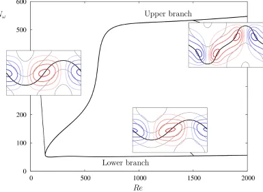
saddle-node bifurcation at Resn≈136, forming upper and lower ECS branches. These solutions,

together with their bifurcation diagram, are shown in figure 1. The primary difference

between the lower and upper branch states lies in the O(1) streaks. The lower branch

streaks undulate with small amplitude aroundy = 0 as opposed to the upper branch streaks

which are more pronounced, nearly spanning the entire domain. The streak deformation

is the result of their interaction with O(ǫ) rolls which are generated by O(ǫ) fluctuations

accumulating around the u0 = 0 contour, that is, around the curve of vanishing streaks.

In the nominally inviscid problem, i.e., the regime of very high Reynolds numbers, this

contour corresponds to the so-called critical layer. The lower branch ECS display

quasi-circular rolls, explaining the sinusoidal shape of the u0 = 0 contour. As the Reynolds

number is decreased toward the saddle-node, the rolls strengthen while maintaining their

nearly circular shape and the undulation amplitude grows. The rolls associated with the

upper branch ECS are more complex: away from the saddle-node they become bimodal

with a pair of local cores replacing the single core along the lower branch. These cores

gradually move apart, toward the extrema of the u0 = 0 contour, considerably deforming

the contour near its extrema (figure 1).

3.2

Modulated states

It is known that a number of different instabilities leading to spatial modulation can arise

Figure 1: Bifurcation diagram for a domain with spanwise periodLz =π and streamwise

wavenumber α = 0.5. The normalized enstrophy: Nω = 1 D

R

Dω

2

1dy dz is shown as a

function of the Reynolds number Re. Here D _{represents the two-dimensional domain and} D =R

D dy dz. The insets represent the lower and upper branch states at Re≈ 1500 and

the solution at the saddle-node Re ≈ _{Resn. The thick black line represents the critical}

layer u0 = 0, and thinner black contours are plotted for u0 = ±0.5,±1. The rolls are

vicinity of saddle-nodes of spatially periodic states [1, 25]. This process has been studied in

detail in the context of the bistable Swift–Hohenberg equation posed on a one-dimensional

domain with a large spatial period [7], and becomes analytically accessible in the context of

the corresponding Ginzburg–Landau equation [15]. The resulting modulational instability

may lead to the development of a hole within the spatially periodic pattern when the

amplitude of modulation becomes so large that the periodic state is invaded by intervals

of the trivial (laminar) state.

With this in mind, we set the domain size to Lz = 4π and look for the formation

of modulated structures at Re ≈ _{Resn. The modulational instabilities described in the}

Swift–Hohenberg equation [7, 15] or in other fluid problems [18, 3] are linear instabilities

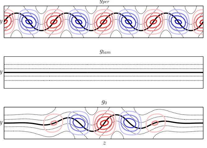
occurring close to the saddle-node. We therefore consider the following initial conditions

g0 for our Newton method:

g0 =

h

1− χ

2

1 + cosz 2

i

gper+

hχ

2

1 + cosz 2

i

glam. (17)

Here gper is the spatially periodic solution at the saddle-node, glam is the homogeneous

laminar solution and χ is a modulation factor. For χ = 0, the initial condition is the

unmodulated periodic state gper; as χ increases spatial modulation with wavelength 4π

(i.e., the spanwise period of the domain) of the pattern develops until χ = 1 where the

modulation is maximum: at z = 0 and z = 4π, the corresponding solution looks like the

laminar profile while at z = 2π its profile takes the form of the saddle-node solution. An

example of such an initial condition is shown in figure 2 together with the exact periodic

state gper and the trivial laminar state glam.

To identify initial conditions that converge to a modulated state, we scanned the (Re, χ)

parameter space. When the Reynolds number is too close to Resn, small values of χ

gper

glam

g0

z y

y y

Figure 2: Relevant solutions, gper and glam, used to generate the initial condition g0 using

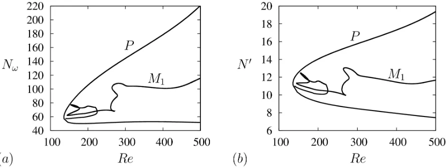
Figure 3: Bifurcation diagram for the modulated state M1 obtained using the initial

con-dition (17) for Re = 140 and χ = 0.2. The quantities represented in (a) are the same as in figure 1 while a measure of the fluctuation energy N′ ₌ 1

D

R

D(v

2 1+w

2

1)dy dz is shown in

(b). The upper branch, lower branch and saddle-node solutions of the periodic states P

are shown in detail in figure 1.

iteration converges to it. However, beyond a threshold value of χ all attempts at

conver-gence failed, the initial condition being structurally too far away from any physical state.

Likewise, values of Rethat were too far fromResn also failed to converge regardless of the

choice ofχ. However, a converged modulated state was found forRe= 140 andχ= 0.2 and

this state was then continued using our continuation algorithm [6] to trace out the branch

M1of the corresponding solutions (figure 3). As expected, the modulated solution emerges

from a bifurcation close to the saddle-node of the branch of spatially periodic states. As

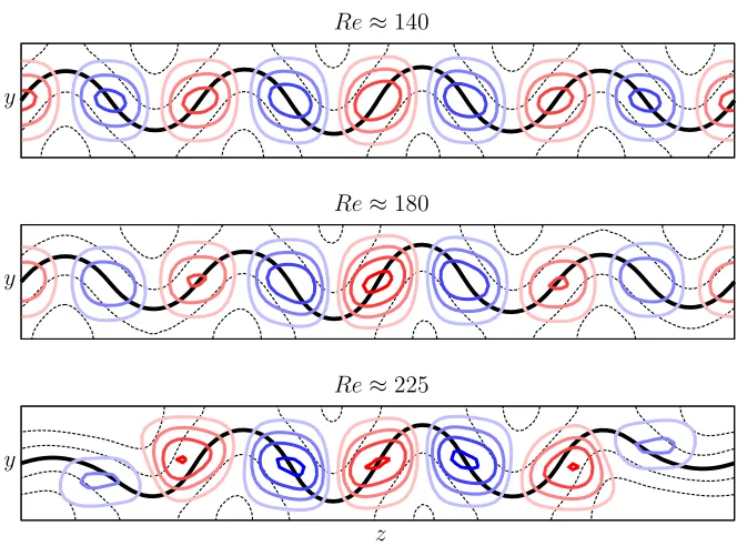
the solution branch is continued, the modulation of the roll amplitude (and therefore of

the streaks) becomes the dominant feature (figure 4): the central (counter-clockwise) roll

becomes stronger while the adjacent rolls become progressively weaker. This is particularly

noticeable close to the first saddle-node of the modulated states at Re ≈_{225. There, the}

ccounter-clockwise roll located at the edge of the (periodic) domain has nearly completely

vanished and the adjacent clockwise rolls (in blue in figure 4) are substantially weaker,

Re≈₁₄₀

Re≈180

Re≈₂₂₅

z y

y y

Figure 4: Progressive modulation of the amplitude of the modulated state as the M1

the displacement of the weaker rolls, we substitute the fluctuation velocities from equation

(15) into equation (14) and obtain:

α2

− ∇2

⊥

p1 =

2

u0

−∇_⊥p· ∇_⊥u0+ǫ∇_⊥u0· ∇ 2

⊥v1⊥

. (18)

Here the term ǫ∇_⊥u0 · ∇ 2

⊥v1⊥ arises from the nature of the asymptotics performed in

Section 2 but ǫ∇2

⊥v1⊥ is never large. However, the presence of u0 in the denominator of

the right side of equation (18) is responsible for the presence of enhanced forcing of the

fluctuations in the vicinity of the contour u0 = 0, implying that fluctuations necessarily

concentrate in the critical region, where they strengthen the rolls and in particular the

counter-clockwise central roll. The weak clockwise rolls at either end deform the u0 = 0

contour less, resulting in a displacement of the contour downward on the left and upward

on the right (figure 4, bottom panel).

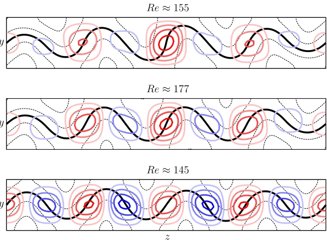
As the branch M1 turns around towards lower values of the Reynolds number near

the Re ≈ _{225 saddle-node, the clockwise rolls weaken while the counter-clockwise rolls}

strengthen. The resulting solution is shown in figure 5 for Re= 155 (top panel). At this

location the M1 branch has a saddle-node; by the next saddle-node (atRe≈177, middle

panel) the central roll is starting to lose its dominance, and this evolution continues towards

the leftmost saddle-node (at Re ≈ _{145, bottom panel) resulting in a roll pattern with}

a rather weak but nonetheless complex modulation structure characterized by a weaker

central roll embedded between a pair of stronger counter-rotating rolls on either side.

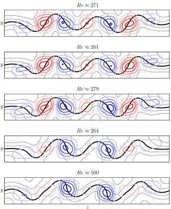
This modulation structure strengthens and by the next saddle-node at Re ≈ _{271 a}

fully-developed double-well modulation is present, centered on the roll pairs on either side of

the counter-clockwise central roll (figure 6). The modulation strenghens the roll pairs on

either side of the central roll while progressively weakening the central roll; this evolution

Re≈₁₅₅

Re≈177

Re≈₁₄₅

z y

y y

Figure 5: Evolution of the M1 branch after its first saddle-node atRe≈225. From top to

bottom: solutions at successive saddle-nodes until the leftmost saddle-node at Re ≈_145.

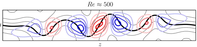
Re≈₂₇₁

Re≈₂₆₁

Re≈₂₇₉

Re≈₂₆₄

Re≈₅₀₀

z y

y y y y

Figure 6: Evolution of theM1 states after their approach to the periodic state (see figure 5).

The solutions are shown, from top to bottom, at the four successive saddle-nodes between

Re= 250 and Re= 300, starting from the one of least energy; the final solution is taken at Re ≈_{500. The corresponding bifurcation diagram is shown in figure 3. The solutions}

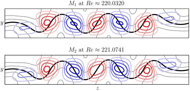
M2atRe≈221.0741

M1atRe≈220.0320

z y

y

Figure 7: NearbyM1 andM2 solutions represented as in previous figures with

streamfunc-tion contours that are multiples of 0.6. These solutions are indicated with a solid dot in the corresponding bifurcation diagram shown in figure 8.

weak clockwise structures towards the outside. The next saddle-node on the left reveals

the presence of dramatic weakening of the outer counter-clockwise rolls while the inner

clockwise rolls strengthen resulting in the steeping of theu0 = 0 contour within the latter,

a process that is progressively enhanced as Re increases (figure 6, bottom panel), in a

manner suggestive of incipient roll-up. The fold at Re ≈ _{145 is therefore responsible}

for the splitting of the one-pulse state into two pulses. Similar splitting of a single-pulse

localized structure occurs in rotating convection [4].

While tracking the M1 state in figure 3, we noticed the presence of a (well-resolved)

sharp angle in the direction of the branch at Re≈_{220 in all the quantities we monitored.}

This type of event might indicate an imperfect bifurcation and therefore the existence of

another branch nearby with similar solutions. We initialized a Newton search with an

M1 solution at Re ≈ 220.0320 and slightly perturbed it by increasing its amplitude and

the Reynolds number. Using this procedure we were able to converge to another kind

of modulated state, labelled M2. The M1 solution we picked together with the M2 state

we converged to are represented in figure 7 to illustrate the similarities and differences

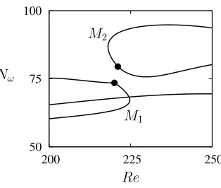
50 75 100

200 225 250

Nω

Re M2

M1

Figure 8: Close-up of the region where the M1 and M2 states approach each other. The

solution on M1 indicated by the solid dot was used to converge to the M2 solution also

indicated by a solid dot.

Figure 9: Bifurcation diagram for the modulated states M1 and M2. The quantities

repre-sented are the same as in figure 3.

bifurcation diagram of the M2 states is shown in figure 9. Continuation of the modulated

statesM2shows that these states are created at a saddle-node atRe≈218. The upper and

lower branches emanating from this saddle-node then have completely different fate. The

upper M2 branch evolves monotonically to larger Reynolds numbers while the modulation

of the amplitude of the rolls increases and the size of the central roll decreases. This

simple evolution is shown in figure 10. The lower branch has a more complex structure,

Re≈₅₀₀

z y

Figure 10: Solution taken along the upper M2 branch at Re ≈ 500. The corresponding

bifurcation diagram is shown in figure 9. The solution is represented as in figure 2 with multiples of 0.6 for the streamfunction contours.

remaining counter-clockwise rolls also weaken leaving a structure dominated by a pair of

strong clockwise rolls. This process manifests itself in the presence of a small loop between

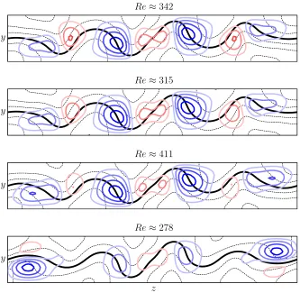
Re ≈ _{315 and Re} ≈ _{342 and terminates near the Re} ≈ _{411 saddle-node in figure 11.}

The branch then turns around and both N and N′ _{increase dramatically. During this}

process the two clockwise rolls near the center of the domain that dominate the flow at

Re ≈ _{411 are swamped by the growth of a pair of clockwise rolls near either side of the}

domain and the associated elimination of counter-clockwise rolls from all but the center

of the domain where a weak counter-clockwise roll persists. It is significant that the new

clockwise rolls that appear are no longer centered on the u0 = 0 contour. This appears to

be a consequence of their proximity in a domain with periodic boundary conditions and

of the resulting roll-up. This incipient roll-up may in turn be responsible for the dramatic

increase in roll and fluctuation energies observed in figure 9. This behavior hints at a

possible failure of the asymptotic approach in this regime, although we have not pushed

the calculations into this regime. We reiterate that all the solutions reported here are fully

Re≈₃₄₂

Re≈₃₁₅

Re≈₄₁₁

Re≈₂₇₈

z y

y y y

Figure 11: Solutions along the lower M2 branch at successive saddle-nodes at Re ≈ 342,

Re ≈ _{315, Re} ≈ _{411 and Re} ≈ _{278. The corresponding bifurcation diagram is shown in}

figure 9. The solution is represented as in figure 2 with multiples of 0.7 for the stream-function contours, except for the Re≈ _{278 saddle-node where multiples of 1.2 have been}

4

Conclusion

In this paper, we have obtained and numerically continued the first spanwise-modulated

states in a reduced model of parallel shear flow, focusing on time-independent solutions

with the symmetryR. These states were found using insight from pattern-forming systems:

the saddle-node of subcritical spatially periodic states in extended systems is known to give

rise to modulational instabilities. We constructed an artificial modulation of the

saddle-node solution and converged it to a modulated state referred to as M1 that we have

successfully continued to unveil a complex bifurcation structure reminiscent of fully

three-dimensional shear flows [22, 12, 19]. Additional solutions such as theM2 modulated states

were identified by perturbing theM1 state close to what looks like an imperfect bifurcation,

and these were likewise continued numerically to substantially different Reynolds numbers.

We mention that states with a shift-reflect symmetry, corresponding to a cross-stream

reflection followed by a half wavelength shift in the streamwise direction, are also expected

to be present [24, 6]. Such solutions are not stationary, however, but drift steadily in the

streamwise direction, i.e., they are traveling waves. We have not computed traveling states

of this type.

The reduced model used for this purpose has been derived based on the scaling

proper-ties of the lower branch state observed in plane Couette flow [29]. The resulting equations

are in effect projected in the streamwise direction on the fundamental and first Fourier

components of the velocity and pressure fields but spanwise and wall-normal directions are

treated as in fully simulated flows. As a result, 3 real fields (u0, ω1 and φ1) and 3 complex

fields (p1,v1 andw1) have to be solved for on aN_y×N_z mesh, whereN_y (resp. N_z) stands

for the number of points in the wall-normal (resp. spanwise) direction. The computation

of such states using a direct numerical solver on the primitive equations typically involves 4

withNx =O(10) at least [23, 12, 19]. The calculations presented here would therefore have

been at least 10 times slower had a fully three-dimensional solver been used. Additional

difficulties arise in the Newton iteration as the number of degrees of freedom increases.

The finding of the modulated states M1 and M2 in a reduced model has several

impli-cations for transitional shear flows. It shows that the reduced model (12)–(15), originally

designed to capture the lower branch solutions, not only captures the upper branch states,

but also bifurcations from these states and even more complex, unconnected states. This

property of the reduced model is expected to provide substantial help in the systematic

study of both extended and spatially localized ECS [24]. In the present study no ECS

localized in the spanwise direction were found but some of the modulated states strongly

suggest that spanwise-localized modulated states do, in fact, exist although no homoclinic

snaking was observed. The M1 and M2 states nearly coincide in an imperfect

bifurca-tion around Re = 220. Had they connected their connection would have given rise to a

branch starting from the saddle-node of the periodic states, spending some time around

Re = 220, before extending monotonically to large Reynolds numbers and resulting in

solutions consisting of a spatially modulated roll pattern with a simple structure. Similar

modulated states that do not snake but instead extend monotonically to large parameter

values have been found in Marangoni convection [1] and studied in detail in the context

of binary fluid convection [20]. These studies, in conjunction with earlier studies of model

equations such as the Swift–Hohenberg equation [7, 9], indicate that in finite domains the

behavior of branches of modulated structures is strongly affected by the spanwise spatial

period imposed on the system, suggesting that for a different choice of this period

homo-clinic snaking may in fact be present in the reduced shear flow model studied here. This

is particularly so for moderately large domains, such as Lz = 4π, as used here. However,

despite this limitation, the present study serves as a proof of concept that reduced models,

been designed for, thereby paving the way for future studies on larger domains at lesser

computational cost.

Acknowledgments: This work was presented at the Turbulent Mixing and Beyond

Workshop at the Abdus Salam International Centre for Theoretical Physics (Trieste, Italy)

in August 2014 by CB. He is grateful for the financial support received from the conference

organizers. The research reported here was supported by the National Science

Founda-tion under grants DMS-1211953 and DMS-1317596 (EK), 0934827 (GPC) and

OCE-0934737 and DMS-1317666 (KJ).

References

[1] P. Assemat, A. Bergeon and E. Knobloch, Fluid Dyn. Res., 40 (2008) 852–876

[2] C. Beaume, Proc. Geophysical Fluid Dynamics Program, Woods Hole Oceanographic

Inst. (2012) 389–412

[3] C. Beaume, E. Knobloch and A. Bergeon, Phys. Fluids, 25 (2013) 114102

[4] C. Beaume, E. Knobloch and A. Bergeon, Phys. Fluids, 25 (2013) 124105

[5] C. Beaume, E. Knobloch, G. P. Chini and K. Julien, Fluid Dyn. Res., 47 (2015) 015504

[6] C. Beaume, G. P. Chini, K. Julien and E. Knobloch, Phys. Rev. E, 91 (2015) 043010

[7] A. Bergeon, J. Burke, E. Knobloch and I. Mercader, Phys. Rev. E, 78 (2008) 046201

[8] M. Chantry, L. S. Tuckerman and D. Barkley, arXiv:1506.05002 (2015)

[9] J. H. P. Dawes, SIAM J. Appl. Dyn. Syst., 8 (2009) 909–930

[10] P. G. Drazin and W. H. Reid, Hydrodynamic Stability, Cambridge University Press

[11] Y. Duguet, P. Schlatter and D. S. Henningson, Phys. Fluids, 21 (2009) 111701

[12] J. F. Gibson, J. Halcrow, and P. Cvitanovi´c, J. Fluid Mech., 638 (2009) 243–266

[13] P. Hall and F. T. Smith, J. Fluid Mech., 227 (1991) 641–666

[14] P. Hall and S. J. Sherwin, J. Fluid Mech., 661 (2010) 178–205

[15] H.-C. Kao and E. Knobloch, Phys. Rev. E, 85 (2012) 026211

[16] G. Kawahara and S. Kida, J. Fluid Mech., 449 (2001) 291–300

[17] G. Kawahara, M. Uhlmann and L. van Veen, Annu. Rev. Fluid Mech., 44 (2012)

203–225

[18] D. Lo Jacono, A. Bergeon and E. Knobloch, Phys. Fluids, 22 (2010) 073601

[19] K. Melnikov, T. Kreilos and B. Eckhardt, Phys. Rev. E, 89 (2014) 043008

[20] I. Mercader, O. Batiste, A. Alonso and E. Knobloch, J. Fluid Mech., 667 (2011)

586–606

[21] M. Nagata, J. Fluid Mech., 217 (1990) 519–527

[22] A. Schmiegel, PhD dissertation, Marburg University (1990)

[23] T. M. Schneider, J. F. Gibson, M. Lagha, F. de Lillo and B. Eckhardt, Phys. Rev. E,

78 (2008) 037301

[24] T. M. Schneider, J. Gibson and J. Burke, Phys. Rev. Lett., 104 (2010) 104501

[25] T. M. Schneider, D. Marinc and B. Eckhardt, J. Fluid Mech., 646 (2010) 441–451

[28] F. Waleffe, J. Fluid Mech., 435 (2001) 93–102