Geometry and dynamics in Gromov hyperbolic metric spaces : With an emphasis on non-proper settings

(1)

arXiv:1409.2155v7 [math.DS] 28 Jun 2016

GEOMETRY AND DYNAMICS IN GROMOV HYPERBOLIC

METRIC SPACES

WITH AN EMPHASIS ON NON-PROPER SETTINGS

Tushar Das

David Simmons

Mariusz Urba´

nski

University of Wisconsin – La Crosse, Department of Mathematics & Statistics, 1725 State Street, La Crosse, WI 54601, USA

E-mail address: tdas@uwlax.edu

URL:https://sites.google.com/a/uwlax.edu/tdas/

University of York, Department of Mathematics, Heslington, York YO10 5DD, UK

E-mail address: David.Simmons@york.ac.uk

URL:https://sites.google.com/site/davidsimmonsmath/

University of North Texas, Department of Mathematics, 1155 Union Circle #311430, Denton, TX 76203-5017, USA

E-mail address: urbanski@unt.edu

(2)

20E08; Secondary 37A45, 22E65, 20M20

Key words and phrases. hyperbolic geometry, Gromov hyperbolic metric space, infinite-dimensional symmetric space, metric tree, Hausdorff dimension, Poincar´e

exponent, Patterson–Sullivan measure, conformal measure, divergence type, geometrically finite group, global measure formula, exact dimensional measure

Abstract. Our monograph presents the foundations of the theory of groups and semigroups acting isometrically on Gromov hyperbolic metric spaces. We make it a point to avoid any assumption of properness/compactness, keep-ing in mind the motivatkeep-ing example ofH∞_{, the infinite-dimensional rank-one}

symmetric space of noncompact type over the reals. We have not skipped over parts that might be thought of as “trivial” extensions of the finite-dimensional/proper theory, as our intuition has turned out to be wrong often enough regarding these matters that we feel it is worth writing everything down explicitly and with an eye to detail. Moreover, we feel that it is a method-ological advantage to have the entire theory presented from scratch, in order to provide a basic reference for the theory.

Though our work unifies and extends a long list of results obtained by many authors, Part 1 of this monograph may be treated as mostly expository. The remainder of this work, some of whose highlights are described in brief below, contains several new methods, examples, and theorems. In Part 2, we introduce a modification of the Poincaré exponent, an invariant of a group which provides more information than the usual Poincaré exponent, which we then use to vastly generalize the Bishop–Jones theorem relating the Hausdorff dimension of the radial limit set to the Poincaré exponent of the underlying semigroup. We construct examples which illustrate the surprising connection between Hausdorff dimension and various notions of discreteness which show up in non-proper settings. Part 3 of the monograph provides a number of examples of groups acting onH∞_{which exhibit a wide range of phenomena not}

to be found in the finite-dimensional theory. Such examples often demonstrate the optimality of our theorems.

(3)

Dedicated to the memory of our friend

Bernd O. Stratmann

Mathematiker

(4)

(5)

3.5. The Gromov product in algebraic hyperbolic spaces 41 3.5.1. The Gromov boundary of an algebraic hyperbolic space 46 3.6. Metrics and metametrics on bordX 48 3.6.1. General theory of metametrics 48 3.6.2. The visual metametric based at a pointw∈X 50 3.6.3. The extended visual metric on bordX 51 3.6.4. The visual metametric based at a pointξ_∈∂X 53

Chapter 4. More about the geometry of hyperbolic metric spaces 59

4.1. Gromov triples 59

4.2. Derivatives 60

4.2.1. Derivatives of metametrics 60

4.2.2. Derivatives of maps 61

4.2.3. The dynamical derivative 63

4.3. The Rips condition 65

4.4. Geodesics in CAT(-1) spaces 67

4.5. The geometry of shadows 73

4.5.1. Shadows in regularly geodesic hyperbolic metric spaces 73 4.5.2. Shadows in hyperbolic metric spaces 74

4.6. Generalized polar coordinates 79

Chapter 5. Discreteness 83

5.1. Topologies on Isom(X) 83

5.2. Discrete groups of isometries 87

5.2.1. Topological discreteness 89

5.2.2. Equivalence in finite dimensions 91

5.2.3. Proper discontinuity 92

(7)

CONTENTS ix

Chapter 6. Classification of isometries and semigroups 95

6.1. Classification of isometries 95

6.1.1. More on loxodromic isometries 97 6.1.2. The story for real hyperbolic spaces 98

6.2. Classification of semigroups 99

6.2.1. Elliptic semigroups 100

6.2.2. Parabolic semigroups 100

6.2.3. Loxodromic semigroups 101

6.3. Proof of the Classification Theorem 103

6.4. Discreteness and focal groups 105

Chapter 7. Limit sets 109

7.1. Modes of convergence to the boundary 109

7.2. Limit sets 112

7.3. Cardinality of the limit set 113

7.4. Minimality of the limit set 114

7.5. Convex hulls 119

7.6. Semigroups which act irreducibly on algebraic hyperbolic spaces 122

7.7. Semigroups of compact type 123

Part 2. The Bishop–Jones theorem 127

Chapter 8. The modified Poincaré exponent 129 8.1. The Poincaré exponent of a semigroup 129 8.2. The modified Poincaré exponent of a semigroup 130 Chapter 9. Generalization of the Bishop–Jones theorem 135

9.1. Partition structures 136

9.2. A partition structure on∂X 141

9.3. Sufficient conditions for Poincar´e regularity 148

Part 3. Examples 155

Chapter 10. Schottky products 157

10.1. Free products 157

10.2. Schottky products 158

10.3. Strongly separated Schottky products 160 10.4. A partition-structure–like structure 168

10.5. Existence of Schottky products 171

Chapter 11. Parabolic groups 175

(8)

11.1.1. The Haagerup property and the absence of a Margulis lemma 176

11.1.2. Edelstein examples 177

11.2. The Poincaré exponent of a finitely generated parabolic group 183 11.2.1. Nilpotent and virtually nilpotent groups 183 11.2.2. A universal lower bound on the Poincaré exponent 185 11.2.3. Examples with explicit Poincaré exponents 186 Chapter 12. Geometrically finite and convex-cobounded groups 193

12.1. Some geometric shapes 193

12.1.1. Horoballs 193

12.1.2. Dirichlet domains 194

12.2. Cobounded and convex-cobounded groups 196 12.2.1. Characterizations of convex-coboundedness 198 12.2.2. Consequences of convex-coboundedness 201

12.3. Bounded parabolic points 201

12.4. Geometrically finite groups 206

12.4.1. Characterizations of geometrical finiteness 207 12.4.2. Consequences of geometrical finiteness 213 12.4.3. Examples of geometrically finite groups 218

Chapter 13. Counterexamples 221

13.1. EmbeddingR-trees into real hyperbolic spaces 222 13.2. Strongly discrete groups with infinite Poincar´e exponent 226 13.3. Moderately discrete groups which are not strongly discrete 226

13.4. Poincar´e irregular groups 228

13.5. Miscellaneous counterexamples 232

Chapter 14. R-trees and their isometry groups 233 14.1. Construction ofR-trees by the cone method 233 14.2. Graphs with contractible cycles 237 14.3. The nearest-neighbor projection onto a convex set 239 14.4. ConstructingR-trees by the stapling method 240 14.5. Examples ofR-trees constructed using the stapling method 245

Part 4. Patterson–Sullivan theory 253

Chapter 15. Conformal and quasiconformal measures 255

15.1. The definition 255

15.2. Conformal measures 256

15.3. Ergodic decomposition 256

(9)

CONTENTS xi

15.4.1. Pointmass quasiconformal measures 260 15.4.2. Non-pointmass quasiconformal measures 261 Chapter 16. Patterson–Sullivan theorem for groups of divergence type 267 16.1. Samuel–Smirnov compactifications 267 16.2. Extending the geometric functions toXb 268

16.3. Quasiconformal measures onXb 270

16.4. The main argument 273

16.5. End of the argument 276

16.6. Necessity of the generalized divergence type assumption 277 16.7. Orbital counting functions of nonelementary groups 279 Chapter 17. Quasiconformal measures of geometrically finite groups 281 17.1. Sufficient conditions for divergence type 281

17.2. The global measure formula 284

17.3. Proof of the global measure formula 289

17.4. Groups for whichµis doubling 295

17.5. Exact dimensionality ofµ 303

17.5.1. Diophantine approximation on Λ 304 17.5.2. Examples and non-examples of exact dimensional measures 308

Appendix A. Open problems 313

Appendix B. Index of defined terms 315

(10)

(11)

List of Figures

3.1.1 A geodesic triangle in anR-tree 27

3.3.1 A quadruple of points in anR-tree 30 3.3.2 Expressing distance via Gromov products in anR-tree 32

3.4.1 A Gromov sequence in anR-tree 34

3.5.1 Relating angle and the Gromov product 42

3.5.2 Bis strongly Gromov hyperbolic 45

3.5.3 A formula for the Busemann function in the half-space model 48

3.6.1 The Hamenst¨adt distance 56

4.2.1 The derivative ofg at_∞ 63

4.3.1 The Rips condition 66

4.4.1 The triangle ∆(x, y1, y2) 69

4.5.1 Shadows in regularly geodesic hyperbolic metric spaces 74

4.5.2 The Intersecting Shadows Lemma 76

4.5.3 The Big Shadows Lemma 77

4.5.4 The Diameter of Shadows Lemma 78

4.6.1 Polar coordinates in the half-space model 79 6.4.1 High altitude implies small displacement in the half-space model 107 7.1.1 Conical convergence to the boundary 110 7.1.2 Converging horospherically but not radially to the boundary 111

9.2.1 The construction of children 142

9.2.2 The setsCn, forn∈Z 143

10.3.1 The strong separation lemma for Schottky products 162 12.1.1 Visualizing horoballs in the ball and half-space models 194 12.1.2 Diameter decay of a ball complement inside a horoball 195

(12)

12.1.3 The Cayley graph of Γ =F2(Z) =hγ1, γ2i 196

12.2.1 Proving that convex-cobounded groups are of compact type 200 12.3.1 The geometry of bounded parabolic points 205 12.4.1 Proving that geometrically finite groups are of compact type 209 12.4.2 Local finiteness of the horoball collection 211 12.4.3 Orbit maps of geometrically finite groups are QI embeddings 215 13.4.1 Geometry of automorphisms of a simplicial tree 229 14.2.1 Triangles in graphs with contractible cycles 239 14.2.2 Triangles in graphs with contractible cycles: general case 239 14.4.1 The consistency condition for stapling metric spaces 242 14.5.1 The Cayley graph ofF2(Z) as a pure Schottky product 248

(13)

Prologue

. . . Cela suffit pour faire comprendre que dans les cinq mémoires des Acta mathematica que j’ai consacrés à l’étude des transcen-dantes fuchsiennes et kleinéennes, je n’ai fait qu’effleurer un su-jet très vaste, qui fournira sans doute aux géomètres l’occasion de nombreuses et importantes découvertes.1

– H. Poincar´e, Acta Mathematica, 5, 1884, p. 278.

The theory of discrete subgroups of real hyperbolic space has a long history. It was inaugurated by Poincar´e, who developed the two-dimensional (Fuchsian) and three-dimensional (Kleinian) cases of this theory in a series of articles published between 1881 and 1884 that included numerous notes submitted to the C. R. Acad. Sci. Paris, a paper at Klein’s request in Math. Annalen, and five memoirs com-missioned by Mittag-Leffler for his then freshly-minted Acta Mathematica. One must also mention the complementary work of the German school that came be-fore Poincar´e and continued well after he had moved on to other areas, viz. that of Klein, Schottky, Schwarz, and Fricke. See [80, Chapter 3] for a brief exposi-tion of this fascinating history, and [79, 63] for more in-depth presentaexposi-tions of the mathematics involved.

We note that in finite dimensions, the theory of higher-dimensional Kleinian groups, i.e., discrete isometry groups of the hyperbolic d-space Hd for d _≥ 4, is markedly different from that in H3 _and _H2_{. For example, the Teichm¨}_uller

the-ory used by the Ahlfors–Bers school (viz. Marden, Maskit, Jørgensen, Sullivan, Thurston, etc.) to study three-dimensional Kleinian groups has no generalization to higher dimensions. Moreover, the recent resolution of the Ahlfors measure con-jecture [3, 43] has more to do with three-dimensional topology than with analysis and dynamics. Indeed, the conjecture remains open in higher dimensions [106, p. 526, last paragraph]. Throughout the twentieth century, there are several instances of theorems proven for three-dimensional Kleinian groups whose proofs extended

1_{This is enough to make it apparent that in these five memoirs in Acta Mathematica which I have}

dedicated to the study of Fuschian and Kleinian transcendants, I have only skimmed the surface of a very broad subject, which will no doubt provide geometers with the opportunity for many important discoveries.

(14)

easily to n dimensions (e.g. [21, 133]), but it seems that the theory of higher-dimensional Kleinian groups was not really considered a subject in its own right until around the 1990s. For more information on the theory of higher-dimensional Kleinian groups, see the survey article [106], which describes the state of the art up to the last decade, emphasizing connections with homological algebra.

But why stop at finiten? Dennis Sullivan, in his IH´ESSeminar on Conformal and Hyperbolic Geometry [164] that ran during the late 1970s and early ’80s, indi-cated a possibility of developing the theory of discrete groups acting by hyperbolic isometries on the open unit ball of a separable infinite-dimensional Hilbert space.2

Later in the early ’90s, Misha Gromov observed the paucity of results regarding such actions in his seminal lectures Asymptotic Invariants of Infinite Groups [86] where he encouraged their investigation in memorable terms: “The spaces like this [infinite-dimensional symmetric spaces] . . . look as cute and sexy to me as their finite dimensional siblings but they have been for years shamefully neglected by geometers and algebraists alike”.

Gromov’s lament had not fallen to deaf ears, and the geometry and represen-tation theory of infinite-dimensional hyperbolic spaceH∞ and its isometry group have been studied in the last decade by a handful of mathematicians, see e.g. [40, 65, 132]. However, infinite-dimensional hyperbolic geometry has come into prominence most spectacularly through the recent resolution of a long-standing conjecture in algebraic geometry due to Enriques from the late nineteenth cen-tury. Cantat and Lamy [47] proved that the Cremona group (i.e. the group of birational transformations of the complex projective plane) has uncountably many non-isomorphic normal subgroups, thus disproving Enriques’ conjecture. Key to their enterprise is the fact, due to Manin [125], that the Cremona group admits a faithful isometric action on a non-separable infinite-dimensional hyperbolic space, now known as the Picard–Manin space.

Our project was motivated by a desire to answer Gromov’s plea by exposing a coherent general theory of groups acting isometrically on the infinite-dimensional hyperbolic space H∞. In the process we came to realize that a more natural do-main for our inquiries was the much larger setting of semigroups acting on Gro-mov hyperbolic metric spaces – that way we could simultaneously answer our own questions about H∞ and construct a theoretical framework for those who are in-terested in more exotic spaces such as the curve graph, arc graph, and arc complex [95, 126, 96] and the free splitting and free factor complexes [89, 27, 104, 96].

2_{This was the earliest instance of such a proposal that we could find in the literature, although}

(15)

PROLOGUE xvii

These examples are particularly interesting as they extend the well-known dic-tionary [26, p.375] between mapping class groups and the groups Out(FN). In another direction, a dictionary is emerging between mapping class groups and Cre-mona groups, see [30, 66]. We speculate that developing the Patterson–Sullivan theory in these three areas would be fruitful and may lead to new connections and analogies that have not surfaced till now.

In a similar spirit, we believe there is a longer story for which this monograph lays the foundations. In general, infinite-dimensional space is a wellspring of out-landish examples and the wide range of new phenomena we have started to uncover has no analogue in finite dimensions. The geometry and analysis of such groups should pique the interests of specialists in probability, geometric group theory, and metric geometry. More speculatively, our work should interact with the ongoing and still nascent study of geometry, topology, and dynamics in a variety of infinite-dimensional spaces and groups, especially in scenarios with sufficient negative cur-vature. Here are three concrete settings that would be interesting to consider: the universal Teichm¨uller space, the group of volume-preserving diffeomorphisms ofR3 or a 3-torus, and the space of K¨ahler metrics/potentials on a closed complex man-ifold in a fixed cohomology class equipped with the Mabuchi–Semmes–Donaldson metric. We have been developing a few such themes. The study of thermodynamics (equilibrium states and Gibbs measures) on the boundaries of Gromov hyperbolic spaces will be investigated in future work [57]. We speculate that the study of stochastic processes (random walks and Brownian motion) in such settings would be fruitful. Furthermore, it would be of interest to develop the theory of discrete isometric actions and limit sets in infinite-dimensional spaces of higher rank.

(16)

(17)

CHAPTER 1

Introduction and Overview

The purpose of this monograph is to present the theory of groups and semi-groups acting isometrically on Gromov hyperbolic metric spaces in full detail as we understand it, with special emphasis on the case of infinite-dimensional alge-braic hyperbolic spaces X = H∞_F , where F denotes a division algebra. We have not skipped over the parts which some would call “trivial” extensions of the finite-dimensional/proper theory, for two main reasons: first, intuition has turned out to be wrong often enough regarding these matters that we feel it is worth writing ev-erything down explicitly; second, we feel it is better methodologically to present the entire theory from scratch, in order to provide a basic reference for the theory, since no such reference exists currently (the closest, [39], has a fairly different emphasis). Thus Part 1 of this monograph should be treated as mostly expository, while Parts 2-4 contain a range of new material. For experts who want a geodesic path to significant theorems, we list here five such results that we prove in this monograph: Theorems 1.2.1 and 1.4.4 provide generalizations of the Bishop–Jones theorem [28, Theorem 1] and the Global Measure Formula [160, Theorem 2], respectively, to Gromov hyperbolic metric spaces. Theorem 1.4.1 guarantees the existence of a

δ-quasiconformal measure for groups of divergence type, even if the space they are acting on is not proper. Theorem 1.4.5 provides a sufficient condition for the exact dimensionality of the Patterson-Sullivan measure of a geometrically finite group, and Theorem 1.4.6 relates the exact dimensionality to Diophantine properties of the measure. However, the reader should be aware that a sharp focus on just these results, without care for their motivation or the larger context in which they are sit-uated, will necessarily preclude access to the interesting and uncharted landscapes that our work has begun to uncover. The remainder of this chapter provides an overview of these landscapes.

Convention 1. The symbols ., &, and ≍ will denote coarse asymptotics; a subscript of + indicates that the asymptotic is additive, and a subscript of ×

indicates that it is multiplicative. For example,A.×,KB means that there exists a constantC >0 (theimplied constant), depending only onK, such thatA≤CB. Moreover, A .+,× B means that there exist constants C1, C2 > 0 so that A ≤ C1B+C2. In general, dependence of the implied constant(s) on universal objects

(18)

such as the metric space X, the group G, and the distinguished point o∈ X (cf. Notation 1.1.5) will be omitted from the notation.

Convention 2. The notation xn −→

n xmeans that xn →xas n→ ∞, while the notationxn−−→

n,+ xmeans that x≍+ lim sup

n→∞ xn≍+lim infn→∞ xn,

and similarly forxn−−→ n,× x.

Convention 3. The symbol⊳is used to indicate the end of a nested proof.

Convention 4. We use the Iverson bracket notation:

[statement] =

  

1 statement true 0 statement false

Convention 5. Given a distinguished point o_∈X, we write

kx_k=d(o, x) and_kg_k=_kg(o)_k.

1.1. Preliminaries

1.1.1. Algebraic hyperbolic spaces. Although we are mostly interested in this monograph in thereal infinite-dimensional hyperbolic spaceH∞_R , the complex and quaternionic hyperbolic spaces H∞_C and H∞_Q are also interesting. In finite dimensions, these spaces constitute (modulo the Cayley hyperbolic plane1) therank one symmetric spaces of noncompact type. In the infinite-dimensional case we retain this terminology by analogy; cf. Remark 2.2.6. For brevity we will refer to a rank one symmetric space of noncompact type as analgebraic hyperbolic space.

There are several equivalent ways to define algebraic hyperbolic spaces; these are known as “models” of hyperbolic geometry. We consider here the hyperboloid model, ball model (Klein’s, not Poincar´e’s), and upper half-space model (which only applies to algebraic hyperbolic spaces defined over the reals, which we will call real hyperbolic spaces), which we denote byHα_F,Bα_F, and Eα, respectively. HereF denotes the base field (either R, C, or Q), and αdenotes a cardinal number. We omit the base field when it is R, and denote the exponent by_∞ when it is #(N), so that H∞ = H#(_R N) is the unique separable infinite-dimensional real hyperbolic space.

The main theorem of Chapter 2 is Theorem 2.3.3, which states that any isom-etry of an algebraic hyperbolic space must be an “algebraic” isomisom-etry. The finite-dimensional case is given as an exercise in Bridson–Haefliger [39, Exercise II.10.21].

1_{We omit all discussion of the Cayley hyperbolic plane}_H2

O, as the algebra involved is too exotic

(19)

1.1. PRELIMINARIES xxi

We also describe the relation between totally geodesic subsets of algebraic hyper-bolic spaces and fixed point sets of isometries (Theorem 2.4.7), a relation which will be used throughout the paper.

Remark 1.1.1. Key to the study of finite-dimensional algebraic hyperbolic spaces is the theory of quasiconformal mappings (e.g., as in Mostow and Pansu’s rigidity theorems [133, 141]). Unfortunately, it appears to be quite difficult to generalize this theory to infinite dimensions. For example, it is an open question [92, p.1335] whether every quasiconformal homeomorphism of Hilbert space is also quasisymmetric.

1.1.2. Gromov hyperbolic metric spaces. Historically, the first motiva-tion for the theory of negatively curved metric spaces came from differential ge-ometry and the study of negatively curved Riemannian manifolds. The idea was to describe the most important consequences of negative curvature in terms of the metric structure of the manifold. This approach was pioneered by Aleksandrov [6], who discovered for each κ _∈ R an inequality regarding triangles in a metric space with the property that a Riemannian manifold satisfies this inequality if and only if its sectional curvature is bounded above byκ, and popularized by Gromov, who called Aleksandrov’s inequality the “CAT(κ) inequality” as an abbreviation for “comparison inequality of Alexandrov–Toponogov” [85, p.106].2A metric space is called CAT(κ) if the distance between any two points on a geodesic triangle is smaller than the corresponding distance on the “comparison triangle” in a model space of constant curvatureκ; see Definition 3.2.1.

The second motivation came from geometric group theory, in particular the study of groups acting on manifolds of negative curvature. For example, Dehn proved that the word problem is solvable for finitely generated Fuchsian groups [64], and this was generalized by Cannon to groups acting cocompactly on manifolds of negative curvature [44]. Gromov attempted to give a geometric characterization of these groups in terms of their Cayley graphs; he tried many definitions (cf. [83,

§6.4], [84, §4]) before converging to what is now known as Gromov hyperbolicity in 1987 [85, 1.1, p.89], a notion which has influenced much research. A metric space is said to beGromov hyperbolic if it satisfies a certain inequality that we call Gromov’s inequality; see Definition 3.3.2. A finitely generated group is then said to be word-hyperbolicif its Cayley graph is Gromov hyperbolic.

2_{It appears that Bridson and Haefliger may be responsible for promulgating the idea that the C in}

(20)

The big advantage of Gromov hyperbolicity is its generality. We give some idea of its scope by providing the following nested list of metric spaces which have been proven to be Gromov hyperbolic:

• CAT(-1) spaces (Definition 3.2.1)

– Riemannian manifolds (both finite- and infinite-dimensional) with sectional curvature≤ −1

∗ Algebraic hyperbolic spaces (Definition 2.2.5)

· Picard–Manin spaces of projective surfaces defined over algebraically closed fields [125], cf. [46, _§3.1]

– R-trees (Definition 3.1.10)

∗ Simplicial trees

· Unweighted simplicial trees

• Cayley metrics (Example 3.1.2) on word-hyperbolic groups

• Green metrics on word-hyperbolic groups [29, Corollary 1.2]

• Quasihyperbolic metrics of uniform domains in Banach spaces [173, The-orem 2.12]

• Arc graphs and curve graphs [95] and arc complexes [126, 96] of finitely punctured oriented surfaces

• Free splitting complexes [89, 96] and free factor complexes [27, 104, 96]

Remark 1.1.2. Many of the above examples admit natural isometric group actions:

• The Cremona group acts isometrically on the Picard–Manin space [125], cf. [46, Theorem 3.3].

• The mapping class group of a finitely punctured oriented surface acts isometrically on its arc graph, curve graph, and arc complex.

• The outer automorphism group Out(FN) of the free group onNgenerators acts isometrically on the free splitting complexFS(FN) and the free factor complex_FF(FN).

(21)

1.1. PRELIMINARIES xxiii

Remark 1.1.4. One of the above examples, namely, Green metrics on word-hyperbolic groups, is a natural class of non-geodesic hyperbolic metric spaces.3

However, Bonk and Schramm proved that all non-geodesic hyperbolic metric spaces can be isometrically embedded into geodesic hyperbolic metric spaces [31, Theorem 4.1], and the equivariance of their construction was proven by Blach`ere, Ha¨ıssinsky, and Mathieu [29, Corollary A.10]. Thus, one could view the assumption of geodesic-ity to be harmless, since most theorems regarding geodesic hyperbolic metric spaces can be pulled back to non-geodesic hyperbolic metric spaces. However, for the most part we also avoid the assumption of geodesicity, mostly for methodological reasons rather than because we are considering any particular non-geodesic hyperbolic met-ric space. Specifically, we felt that Gromov’s definition of hyperbolicity in metmet-ric spaces is a “deep” definition whose consequences should be explored independently of such considerations as geodesicity. We do make the assumption of geodesic-ity in Chapter 12, where it seems necessary in order to prove the main theorems. (The assumption of geodesicity in Chapter 12 can for the most part be replaced by the weaker assumption of almost geodesicity [31, p.271], but we felt that such a presentation would be more technical and less intuitive.)

We now introduce a list of standing assumptions and notations. They apply to all chapters except for Chapters 2, 3, and 5 (see also§4.1).

Notation1.1.5. Throughout the introduction,

• X is a Gromov hyperbolic metric space (cf. Definition 3.3.2),

• ddenotes the distance function ofX,

• ∂X denotes the Gromov boundary ofX, and bordX denotes the bordifi-cation bordX=X_∪∂X (cf. Definition 3.4.2),

• Ddenotes a visual metric on∂X with respect to a parameterb >1 and a distinguished pointo_∈X (cf. Proposition 3.6.8). By definition, a visual metric satisfies the asymptotic

(1.1.1) Db,o(ξ, η)≍× b−hξ|ηio,

whereh·|·idenotes the Gromov product (cf. (3.3.2)).

• Isom(X) denotes the isometry group ofX. Also,G_≤Isom(X) will mean that Gis a subgroup of Isom(X), while GIsom(X) will mean thatG

is a subsemigroup of Isom(X).

A prime example to have in mind is the special case where X is an infinite-dimensional algebraic hyperbolic space, in which case the Gromov boundary ∂X 3_{Quasihyperbolic metrics on uniform domains in Banach spaces can also fail to be geodesic, but}

(22)

can be identified with the natural boundary ofX (Proposition 3.5.3), and we can setb=eand get equality in (1.1.1) (Observation 3.6.7).

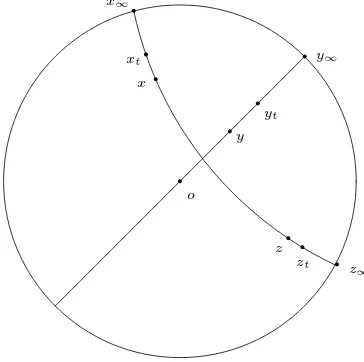
Another important example of a hyperbolic metric space that we will keep in our minds is the case of R-trees alluded to above. R-trees are a generalization of simplicial trees, which in turn are a generalization of unweighted simplicial trees, also known as “Z-trees” or just “trees”. R-trees are worth studying in the context of hyperbolic metric spaces for two reasons: first of all, they are “prototype spaces” in the sense that any finite set in a hyperbolic metric space can be roughly iso-metrically embedded into anR-tree, with a roughness constant depending only on the cardinality of the set [77, pp.33-38]; second of all,R-trees can be equivariantly embedded into infinite-dimensional real hyperbolic space H∞ (Theorem 13.1.1), meaning that any example of a group acting on anR-tree can be used to construct an example of the same group acting on H∞_. _R_{-trees are also much simpler to}

understand than general hyperbolic metric spaces: for any finite set of points, one can draw out a list of all possible diagrams, and then the set of distances must be determined from one of these diagrams (cf. e.g., Figure 3.3.1).

Besides introducingR-trees, CAT(-1) spaces, and hyperbolic metric spaces, the following things are done in Chapter 3: construction of the Gromov boundary

∂X and analysis of its basic topological properties (Section 3.4), proof that the Gromov boundary of an algebraic hyperbolic space is equal to its natural boundary (Proposition 3.5.3), and the construction of various metrics and metametrics on the boundary ofX(Section 3.6). None of this is new, although the idea of a metametric (due to Väisälä [172,_§4]) is not very well known.

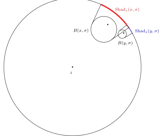
In Chapter 4, we go more into detail regarding the geometry of hyperbolic metric spaces. We prove the geometric mean value theorem for hyperbolic metric spaces (Section 4.2), the existence of geodesic rays connecting two points in the boundary of a CAT(-1) space (Proposition 4.4.4), and various geometrical theorems regarding the sets

Shadz(x, σ) :={ξ∈∂X :hx|ξiz ≤σ},

(23)

1.1. PRELIMINARIES xxv

1.1.3. Discreteness. The first step towards extending the theory of Kleinian groups to infinite dimensions (or more generally to hyperbolic metric spaces) is to define the appropriate class of groups to consider. This is less trivial than might be expected. Recalling that ad-dimensional Kleinian group is defined to be a discrete subgroup of Isom(Hd_{), we would want to define an infinite-dimensional Kleinian} group to be a discrete subgroup of Isom(H∞_{). But what does it mean for a subgroup}

of Isom(H∞_{) to be discrete? In finite dimensions, the most natural definition is}

to call a subgroup discrete if it is discrete relative to the natural topology on Isom(Hd_{); this definition works well since Isom(H}d_{) is a Lie group. But in infinite} dimensions and especially in more exotic spaces, many applications require stronger hypotheses (e.g., Theorem 1.2.1, Chapter 12). In Chapter 5, we discuss several potential definitions of discreteness, which are inequivalent in general but agree in the case of finite-dimensional spaceX=Hd _{(Proposition 5.2.10):}

Definitions 5.2.1 and 5.2.6. FixG≤Isom(X).

• Gis calledstrongly discrete (SD)if for every bounded setB_⊆X, we have #_{g_∈G:g(B)_∩B₆=}<∞.

• Gis called moderately discrete (MD) if for every x∈X, there exists an open setU containingxsuch that

#_{g_∈G:g(U)_∩U ₆=}<∞.

• Gis calledweakly discrete (WD) if for everyx_∈X, there exists an open setU containingxsuch that

g(U)_∩U ₆=⇒g(x) =x.

• Gis calledCOT-discrete (COTD) if it is discrete as a subset of Isom(X) when Isom(X) is given the compact-open topology (COT).

• If X is an algebraic hyperbolic space, then G is called UOT-discrete (UOTD) if it is discrete as a subset of Isom(X) when Isom(X) is given the uniform operator topology (UOT; cf. Section 5.1).

As our naming suggests, the condition of strong discreteness is stronger than the condition of moderate discreteness, which is in turn stronger than the condition of weak discreteness (Proposition 5.2.4). Moreover, any moderately discrete group is COT-discrete, and any weakly discrete subgroup of Isom(H∞_{) is COT-discrete}

(24)

subgroup of Isom(H∞_{)”. However, in this monograph we will be interested in the}

consequences of all the different notions of discreteness, as well as the interactions between them.

Remark 1.1.6. Strongly discrete groups are known in the literature as met-rically proper, and moderately discrete groups are known aswandering. However, we prefer our terminology since it more clearly shows the relationship between the different notions of discreteness.

1.1.4. The classification of semigroups. After clarifying the different types of discreteness which can occur in infinite dimensions, we turn to the question of classification. This question makes sense both for individual isometries and for en-tire semigroups.4_{Historically, the study of classification began in the 1870s when}

Klein proved a theorem classifying isometries ofH2 _{and attached the words}

“ellip-tic”, “parabolic”, and “hyperbolic” to these classifications. Elliptic isometries are those which have at least one fixed point in the interior, while parabolic isometries have exactly one fixed point, which is a neutral fixed point on the boundary, and hyperbolic isometries have two fixed points on the boundary, one of which is at-tracting and one of which is repelling. Later, the word “loxodromic” was used to refer to isometries in H3 which have two fixed points on the boundary but which are geometrically “screw motions” rather than simple translations. In what follows we use the word “loxodromic” to refer to all isometries of Hn (or more generally a hyperbolic metric space) with two fixed points on the boundary – this is analogous to calling a circle an ellipse. Our real reason for using the word “loxodromic” in this instance, rather than “hyperbolic”, is to avoid confusion with the many other meanings of the word “hyperbolic” that have entered usage in various scenarios.

To extend this classification from individual isometries to groups, we call a group “elliptic” if its orbits are bounded, “parabolic” if it has a unique neutral global fixed point on the boundary, and “loxodromic” if it contains at least one loxodromic isometry. The main theorem of Chapter 6 (viz. Theorem 6.2.3) is that every subsemigroup of Isom(X) is either elliptic, parabolic, or loxodromic.

Classification of groups has appeared in the literature in various contexts, from Eberlein and O’Neill’s results regarding visiblility manifolds [69], through Gro-mov’s remarks about groups acting on strictly convex spaces [83,§3.5] and word-hyperbolic groups [85,_§3.1], to the more general results of Hamann [88, Theorem

4_{In Chapters 6-10, we work in the setting of semigroups rather than groups. Like dropping the}

(25)

1.1. PRELIMINARIES xxvii

2.7], Osin [140, §3], and Caprace, de Cornulier, Monod, and Tessera [48, §3.A] regarding geodesic hyperbolic metric spaces.5_{Many of these theorems have similar}

statements to ours ([88] and [48] seem to be the closest), but we have not kept track of this carefully, since our proof appears to be sufficiently different to warrant independent interest anyway.

After proving Theorem 6.2.3, we discuss further aspects of the classification of groups, such as the further classification of loxodromic groups given in _§6.2.3: a loxodromic group is called “lineal”, “focal”, or “of general type” according to whether it has two, one, or zero global fixed points, respectively. (This terminology was introduced in [48].) The “focal” case is especially interesting, as it represents a class of nonelementary groups which have global fixed points.6We show that certain classes of discrete groups cannot be focal (Proposition 6.4.1), which explains why such groups do not appear in the theory of Kleinian groups. On the other hand, we show that in infinite dimensions, focal groups can have interesting limit sets even though they satisfy only a weak form of discreteness; cf. Remark 13.4.3.

1.1.5. Limit sets. An important invariant of a Kleinian groupGis its limit set Λ = ΛG, the set of all accumulation points of the orbit of any point in the interior. By putting an appropriate topology on the bordification of our hyperbolic metric spaceX (§3.4.2), we can generalize this definition to an arbitrary subsemi-group of Isom(X). Many results generalize relatively straightforwardly7_{to this new}

context, such as the minimality of the limit set (Proposition 7.4.1) and the connec-tion between classificaconnec-tion and the cardinality of the limit set (Proposiconnec-tion 7.3.1). In particular, we call a semigroupelementary if its limit set is finite.

In general, the convex hull of the limit set may need to be replaced by a quasiconvex hull (cf. Definition 7.5.1), since in certain cases the convex hull does not accurately reflect the geometry of the group. Indeed, Ancona [9, Corollary C] and Borbely [32, Theorem 1] independently constructed examples of CAT(-1) three-manifoldsX for which there exists a pointξ_∈∂X such that the convex hull of any neighborhood ofξis equal to bordX. Although in a non-proper setting the limit set may no longer be compact, compactness of the limit set is a reasonable geometric condition that is satisfied for many examples of subgroups of Isom(H∞₎

5_{We remark that the results of [}₄₈_,_§_{3.A] can be generalized to non-geodesic hyperbolic metric}

spaces by using the Bonk–Schramm embedding theorem [31, Theorem 4.1] (see also [29, Corollary A.10]).

6_{Some sources (e.g. [}₁₄₈_,_§_{5.5]) define nonelementarity in a way such that global fixed points are}

automatically ruled out, but this is not true of our definition (Definition 7.3.2).

7_{As is the case for many of our results, the classical proofs use compactness in a crucial way –}

(26)

(e.g. Examples 13.2.2, 13.4.2). We call this condition compact type (Definition 7.7.1).

1.2. The Bishop–Jones theorem and its generalization

The term Poincaré series classically referred to a variety of averaging pro-cedures, initiated by Poincaré in his aforementioned Acta memoirs, with a view towards uniformization of Riemann surfaces via the construction of automorphic forms. Given a Fuchsian group Γ and a rational functionH :bC_→Cbwith no poles on∂B2, Poincaré proved that for everym_≥2 the series

X

γ∈Γ

H(γ(z))(γ′(z))m

(defined for z outside the limit set of Γ) converges uniformly to an automorphic form of dimensionm; see [63, p.218]. Poincaré called these series “θ-fuchsian series of orderm”, but the name “Poincaré series” was later used to refer to such objects.8 The question of for whichm <2 the Poincaré series still converges was investigated by Schottky, Burnside, Fricke, and Ritter; cf. [2, pp.37-38].

In what would initially appear to be an unrelated development, mathematicians began to study the “thickness” of the limit set of a Fuchsian group: in 1941 Myrberg [135] showed that the limit set Λ of a nonelementary Fuchsian group has positive logarithmic capacity; this was improved by Beardon [17] who showed that Λ has positive Hausdorff dimension, thus deducing Myrberg’s result as a corollary (since positive Hausdorff dimension implies positive logarithmic capacity for compact sub-sets ofR2_{[166]). The connection between this question and the Poincar´e series was}

first observed by Akaza, who showed that if G is a Schottky group for which the Poincaré series converges in dimensions, then the Hausdorffs-dimensional measure of Λ is zero [5, Corollary of Theorem A]. Beardon then extended Akaza’s result to finitely generated Fuchsian groups [19, Theorem 5], as well as defining theexponent of convergence (orPoincaré exponent)δ= δG of a Fuchsian or Kleinian group to be the infimum ofsfor which the Poincaré series converges in dimensions(cf. Def-inition 8.1.1 and [18]). The reverse direction was then proven by Patterson [142] using a certain measure on Λ to produce the lower bound, which we will say more about below in_§1.4. Patterson’s results were then generalized by Sullivan [161] to the setting of geometrically finite Kleinian groups. The necessity of the geometri-cal finiteness assumption was demonstrated by Patterson [143], who showed that there exist Kleinian groups of the first kind (i.e. with limit set equal to ∂Hd_{) with}

8_{The modern definition of Poincar´}_{e series (cf. Definition 8.1.1) is phrased in terms of hyperbolic}

geometry rather than complex analysis, but it agrees with the special case of Poincar´e’s original definition which occurs whenH≡1 and z= 0, with the caveat thatγ′

(z)m _{should be replaced} by|γ′

(27)

1.2. THE BISHOP–JONES THEOREM AND ITS GENERALIZATION xxix

arbitrarily small Poincar´e exponent [143] (see also [100] or [157, Example 8] for an earlier example of the same phenomenon).

Generalizing these theorems beyond the geometrically finite case requires the introduction of theradial anduniformly radial limit sets. In what follows, we will denote these sets by Λr and Λur, respectively. Note that the radial and uniformly

radial limit sets as well as the Poincar´e exponent can all (with some care) be defined for general hyperbolic metric spaces; see Definitions 7.1.2, 7.2.1, and 8.1.1. The radial limit set was introduced by Hedlund in 1936 in his analysis of transitivity of horocycles [90, Theorem 2.4].

After some intermediate results [72, 158], Bishop and Jones [28, Theorem 1] generalized Patterson and Sullivan by proving that if G is a nonelementary Kleinian group, then dimH(Λr) = dimH(Λur) = δ.9 Further generalization was

made by Paulin [144], who proved the equation dimH(Λr) =δ in the case where G_≤Isom(X), andX is either a word-hyperbolic group, a CAT(-1) manifold, or a locally finite unweighted simplicial tree which admits a discrete cocompact action. We may now state the first major theorem of this monograph, which generalizes all the aforementioned results:

Theorem 1.2.1. Let G_≤Isom(X)be a nonelementary group. Suppose either that

(1) Gis strongly discrete,

(2) X is a CAT(-1) space andGis moderately discrete,

(3) X is an algebraic hyperbolic space and Gis weakly discrete, or that (4) X is an algebraic hyperbolic space andGacts irreducibly (cf. Section 7.6)

and is COT-discrete. Then there existsσ >0 such that

(1.2.1) dimH(Λr) = dimH(Λur) = dimH(Λur∩Λr,σ) =δ

(cf. Definitions 7.1.2 and 7.2.1 for the definition of Λr,σ); moreover, for every 0< s < δ there existτ >0 and an Ahlforss-regular10_set

Js⊆Λur,τ ∩Λr,σ. For the proof of Theorem 1.2.1, see the comments below Theorem 1.2.3.

Remark. We note that weaker versions of Theorem 1.2.1 already appeared in [58] and [73], each of which has a two-author intersection with the present paper. In particular, case (1) of Theorem 1.2.1 appeared in [73] and the proofs of Theorem 1.2.1 and [73, Theorem 5.9] contain a number of redundancies. This was due to the

9_{Although Bishop and Jones’ theorem only states that dimH(Λr) =} _{δ, they remark that their}

proof actually shows that dimH(Λur) =δ[28, p.4].

10_{Recall that a measure} _µ_{on a metric space}_Z _{is called}_Ahlfors _s_-regular _{if for all} _z_∈ _Z _and

0 < r ≤1, we have that µ(B(z, r)) ≍× rs. The topological support of an Ahlforss-regular

(28)

fact that we worked on two projects which, despite having fundamentally different objectives, both required essentially the same argument to produce “large, nice” subsets of the limit set: in the present monograph, this argument forms the core of the proof of our generalization of the Bishop–Jones theorem, while in [73], the main use of the argument is in proving the full dimension of the set of badly approximable points, in two different senses of the phrase “badly approximable” (approximation by the orbits of distinguished points, vs. approximation by rational vectors in an ambient Euclidean space). There are also similarities between the proof of Theorem 1.2.1 and the proof of the weaker version found in [58, Theorem 8.13], although in this case the presentation is significantly different. However, we remark that the main Bishop–Jones theorem of this monograph, Theorem 1.2.3, is significantly more powerful than both [73, Theorem 5.9] and [58, Theorem 8.13].

Remark. The “moreover” clause is new even in the case which Bishop and Jones considered, demonstrating that the limit set Λur can be approximated by

subsets which are particularly well distributed from a geometric point of view. It does not follow from their theorem since a set could have large Hausdorff dimension without having any closed Ahlfors regular subsets of positive dimension (much less full dimension); in fact it follows from the work of Kleinbock and Weiss [116] that the set of well approximable numbers forms such a set.11_{In [73], a slight}

strength-ening of this clause was used to deduce the full dimension of badly approximable vectors in the radial limit set of a Kleinian group [73, Theorem 9.3].

Remark. It is possible for a group satisfying one of the hypotheses of Theorem 1.2.1 to also satisfyδ=_∞(Examples 13.2.1-13.3.3 and 13.5.1-13.5.2);12_{note that}

Theorem 1.2.1 still holds in this case.

Remark. A natural question is whether (1.2.2) can be improved by showing that there exists someσ >0 for which dimH(Λur,σ) =δ (cf. Definitions 7.1.2 and 7.2.1 for the definition of Λur,σ). The answer is negative. For a counterexample, takeX = H2 _and _G_{= SL}

2(Z)≤ Isom(X); then for all σ > 0 there exists ε > 0

such that Λur,σ ⊆ BA(ε), where BA(ε) denotes the set of all real numbers with Lagrange constant at most 1/ε. (This follows e.g. from making the correspondence in [73, Observation 1.15 and Proposition 1.21] explicit.) It is well-known (see e.g. [118] for a more precise result) that dimH(BA(ε))<1 for allε >0, demonstrating that dimH(Λur,σ)<1 =δ.

11_{It could be objected that this set is not closed and therefore should not constitute a}

counterex-ample. However, since it has full measure, it has closed subsets of arbitrarily large measure (which in particular still have dimension 1).

12_{For the parabolic examples, take a Schottky product (Definition 10.2.1) with a lineal group}

(29)

1.2. THE BISHOP–JONES THEOREM AND ITS GENERALIZATION xxxi

Remark. Although Theorem 1.2.1 computes the Hausdorff dimension of the radial and uniformly radial limit sets, there are many other subsets of the limit set whose Hausdorff dimension it does not compute, such as the horospherical limit set (cf. Definitions 7.1.3 and 7.2.1) and the “linear escape” sets (Λα)α∈(0,1)[122]. We

plan on discussing these issues at length in [57].

Finally, let us also remark that the hypotheses (1) - (4) cannot be weakened in any of the obvious ways:

Proposition1.2.2. We may have dimH(Λr)< δ even if:

(1) Gis moderately discrete (even properly discontinuous) (Example 13.4.4). (2) X is a proper CAT(-1) space andGis weakly discrete (Example 13.4.1). (3) X =H∞ andGis COT-discrete (Example 13.4.9).

(4) X =H∞ andGis irreducible and UOT-discrete (Example 13.4.2). (5) X =H2 (Example 13.4.5).

In each case the counterexample group Gis of general type (see Definition 6.2.13) and in particular is nonelementary.

1.2.1. The modified Poincaré exponent. The examples of Proposition 1.2.2 illustrate that the Poincaré exponent does not always accurately calculate the Hausdorff dimension of the radial and uniformly radial limit sets. In Chapter 8 we introduce a modified version of the Poincaré exponent which succeeds at accu-rately calculating dimH(Λr) and dimH(Λur) for all nonelementary groupsG. (When G is an elementary group, dimH(Λr) = dimH(Λur) = 0, so there is no need for a

sophisticated calculation in this case.) Some motivation for the following definition is given in _§8.2.

Definition 8.2.3. LetGbe a subsemigroup of Isom(X).

• For each setS⊆X ands≥0, let Σs(S) =

X

x∈S

b−skxk

∆(S) ={s≥0 : Σs(S) =∞}

δ(S) = sup ∆(S). • Themodified Poincar´e set ofGis the set

(8.2.2) ∆eG =

\

ρ>0 \

Sρ

∆(Sρ),

where the second intersection is taken over all maximalρ-separated sets

(30)

• The numberδeG= sup∆eG is called themodified Poincar´e exponent ofG. If δeG ∈ ∆eG, we say that G is of generalized divergence type,13 while if

e

δG∈[0,∞)\∆eG, we say thatGis of generalized convergence type. Note that if eδG =∞, thenGis neither of generalized convergence type nor of generalized divergence type.

We may now state the most powerful version of our Bishop–Jones theorem:

Theorem 1.2.3 (Proven in Chapter 9). Let GIsom(X)be a nonelementary semigroup. There exists σ >0 such that

(1.2.2) dimH(Λr) = dimH(Λur) = dimH(Λur∩Λr,σ) =eδ.

Moreover, for every 0 < s < eδ there exist τ > 0 and an Ahlfors s-regular set

Js⊆Λur,τ∩Λr,σ.

Theorem 1.2.1 can be deduced as a corollary of Theorem 1.2.3; specifically, Propositions 8.2.4(ii) and 9.3.1 show that any group satisfying the hypotheses of Theorem 1.2.1 satisfies δ= eδ, and hence for such a group (1.2.2) implies (1.2.1). On the other hand, Proposition 1.2.2 shows that Theorem 1.2.3 applies in many cases where Theorem 1.2.1 does not.

We call a group Poincaré regular if its Poincaré exponent δ and modified Poincaré exponenteδ are equal. In this language, Proposition 9.3.1/Theorem 1.2.1 describes sufficient conditions for a group to be Poincaré regular, and Proposition 1.2.2 provides a list of examples of groups which are Poincaré irregular.

Though Theorem 1.2.3 requiresGto be nonelementary, the following corollary does not:

Corollary 1.2.4. Fix GIsom(X). Then for someσ >0, (1.2.3) dimH(Λr) = dimH(Λur) = dimH(Λur∩Λr,σ).

Proof. IfGis nonelementary, then (1.2.3) follows from (1.2.2). On the other hand, ifGis elementary, then all three terms of (1.2.3) are equal to zero.

1.3. Examples

A theory of groups acting on infinite-dimensional space would not be complete without some good ways to construct examples. Techniques used in the finite-dimensional setting, such as arithmetic construction of lattices and Dehn surgery, do not work in infinite dimensions. (The impossibility of constructing lattices in

13_{We use the adjective “generalized” rather than “modified” because all groups of}

(31)

1.3. EXAMPLES xxxiii

Isom(H∞_{) as a direct limit of arithmetic lattices in Isom(}_Hd_{) is due to known lower} bounds on the covolumes of such lattices which blow up as the dimension goes to infinity; see Proposition 12.2.3 below.) Nevertheless, there is a wide variety of groups acting onH∞, including many examples of actions which have no analogue in finite dimensions.

1.3.1. Schottky products. The most basic tool for constructing groups or semigroups on hyperbolic metric spaces is the theory of Schottky products. This theory was created by Schottky in 1877 when he considered the Fuchsian group generated by a finite collection of loxodromic isometriesgi described by a disjoint collection of balls B_i+ and B_i− with the property that gi(H2\B−i ) = B

+

i . It was extended further in 1883 by Klein’s Ping-Pong Lemma, and used effectively by Patterson [143] to construct a “pathological” example of a Kleinian group of the first kind with arbitrarily small Poincar´e exponent.

We consider here a quite general formulation of Schottky products: a collection of subsemigroups of Isom(X) is said to be in Schottky position if open sets can be found satisfying the hypotheses of the Ping-Pong lemma whose closure is not equal to X (cf. Definition 10.2.1). This condition is sufficient to guarantee that the product of groups in Schottky position (called aSchottky product) is always COT-discrete, but stronger hypotheses are necessary in order to prove stronger forms of discreteness. There is a tension here between hypotheses which are strong enough to prove useful theorems and hypotheses which are weak enough to admit interesting examples. For the purposes of this monograph we make a fairly strong assumption (the strong separation condition, Definition 10.3.1), one which rules out infinitely generated Schottky groups whose generating regions have an accumulation point (for example, infinitely generated Schottky subgroups of Isom(Hd_{)). However, we} plan on considering weaker hypotheses in future work [57].

One theorem of significance in Chapter 10 is Theorem 10.4.7, which relates the limit set of a Schottky product to the limit set of its factors together with the image of a Cantor set ∂Γ under a certain symbolic coding map π : ∂Γ _→ ∂X. As a consequence, we deduce that the properties of compact type and geometri-cal finiteness are both preserved under finite strongly separated Schottky products (Corollary 10.4.8 and Proposition 12.4.19, respectively). A result analogous to The-orem 10.4.7 in the setting of infinite alphabet conformal iterated function systems can be found in [128, Lemma 2.1].

(32)

1.3.2. Parabolic groups. A major point of departure where the theory of subgroups of Isom(H∞_{) becomes significantly different from the finite-dimensional}

theory is in the study of parabolic groups. As a first example, knowing that a group admits a discrete parabolic action on Isom(X) places strong restrictions on the al-gebraic properties of the group ifX=Hd_F, but not ifX =H∞_F . Concretely, discrete parabolic subgroups of Isom(Hd

F) are always virtually nilpotent (virtually abelian ifF=R), but any group with the Haagerup property admits a parabolic strongly discrete action onH∞ _{(indeed, this is a reformulation of one of the equivalent}

def-initions of the Haagerup property; cf. [50, p.1, (4)]). Examples of groups with the Haagerup property include all amenable groups and free groups. Moreover, strongly discrete parabolic subgroups of Isom(H∞_{) need not be finitely generated;}

cf. Example 11.2.20.

Moving to infinite dimensions changes not only the algebraic but also the geo-metric properties of parabolic groups. For example, the cyclic group generated by a parabolic isometry may fail to be discrete in any reasonable sense (Example 11.1.12), or it may be discrete in some senses but not others (Example 11.1.14). The Poincaré exponent of a parabolic subgroup of Isom(Hd_F) is always a half-integer [54, Proof of Lemma 3.5], but the situation is much more complicated in infinite dimensions. We prove a general lower bound on the Poincaré exponent of a para-bolic subgroup of Isom(X) for any hyperbolic metric space X, depending only on the algebraic structure of the group (Theorem 11.2.6); in particular, the Poincaré exponent of a parabolic action ofZk on a hyperbolic metric space is always at least

k/2. Of course, it is well-known that all parabolic actions of Zk on Hd achieve equality. By contrast, we show that for every δ > k/2 there exists a parabolic action ofZk _on_H∞_{whose Poincar´e exponent is equal to}_δ_{(Theorem 11.2.11).}

1.3.3. Geometrically finite and convex-cobounded groups. It has been known for a long time that every finitely generated Fuchsian group has a finite-sided convex fundamental domain (e.g. [108, Theorem 4.6.1]). This result does not gen-eralize beyond two dimensions (e.g. [25, 102]), but subgroups of Isom(H3_{) with}

finite-sided fundamental domains came to be known asgeometrically finite groups. Several equivalent definitions of geometrical finiteness in the three-dimensional set-ting became known, for example Beardon and Maskit’s condition that the limit set is the union of the radial limit set Λr with the set Λbp of bounded parabolic points

(33)

1.3. EXAMPLES xxxv

[12]), so a higher-dimensional Kleinian group is said to begeometrically finiteif it satisfies any of Bowditch’s five equivalent conditions (GF1)-(GF5).

In infinite dimensions, conditions (GF3)-(GF5) are no longer useful (cf. Remark 12.4.6), but appropriate generalizations of conditions (GF1) (convex core is equal to a compact set minus a finite number of cusp regions) and (GF2) (the Beardon– Maskit formula Λ = Λr∪Λbp) are still equivalent for groups of compact type. In fact,

(GF1) is equivalent to (GF2) + compact type (Theorem 12.4.5). We define a group to begeometrically finiteif it satisfies the appropriate analogue of (GF1) (Definition 12.4.1). A large class of examples of geometrically finite subgroups of Isom(H∞₎

is furnished by combining the techniques of Chapters 10 and 11; specifically, the strongly separated Schottky product of any finite collection of parabolic groups and/or cyclic loxodromic groups is geometrically finite (Corollary 12.4.20).

It remains to answer the question of what can be proven about geometrically finite groups. This is a quite broad question, and in this monograph we content ourselves with proving two theorems. The first theorem, Theorem 12.4.14, is a generalization of the Milnor–Schwarz lemma [39, Proposition I.8.19] (see also The-orem 12.2.12), and describes both the algebra and geometry of a geometrically finite group G: firstly, G is generated by a finite subset F ⊆ G together with a finite collection of parabolic subgroupsGξ (which are not necessarily finitely generated, e.g. Example 11.2.20), and secondly, the orbit mapg 7→g(o) is a quasi-isometric embedding from (G, dG) intoX, wheredG is a certain weighted Cayley metric (cf. Example 3.1.2 and (12.4.6)) onG whose generating set isF_∪S_ξGξ. As a conse-quence (Corollary 12.4.17), we see that if the groups Gξ, ξ ∈Λbp, are all finitely

generated, then G is finitely generated, and if these groups have finite Poincar´e exponent, then Ghas finite Poincar´e exponent.

1.3.4. Counterexamples. A significant class of subgroups of Isom(H∞_{) that}

has no finite-dimensional analogue is provided by the Burger–Iozzi–Monod (BIM) representation theorem [40, Theorem 1.1], which states that any unweighted sim-plicial tree can be equivariantly and quasi-isometrically embedded into an infinite-dimensional real hyperbolic space, with a precise relation between distances in the domain and distances in the range. We call the embeddings provided by their theoremBIM embeddings, and the corresponding homomorphisms provided by the equivariance we callBIM representations. We generalize the BIM embedding theo-rem to the case whereX is a separableR-tree rather than an unweighted simplicial tree (Theorem 13.1.1).

(34)

us to translate counterexamples in R-trees into counterexamples in H∞_{. For}

ex-ample, if Γ is the free group on two elements acting on its Cayley graph, then the image of Γ under a BIM representation provides a counterexample both to an infinite-dimensional analogue of Margulis’s lemma (cf. Example 13.1.5) and to an infinite-dimensional analogue of I. Kim’s theorem regarding length spectra of finite-dimensional algebraic hyperbolic spaces (cf. Remark 13.1.6).

Most of the other examples in Chapter 13 are concerned with our various notions of discreteness (cf. §1.1.3 above), the notion of Poincar´e regularity (i.e. whether or not δ=eδ), and the relations between them. Specifically, we show that the only relations are the relations which were proven in Chapter 5 and Proposi-tion 9.3.1, as summarized in Table 1, p.93. Perhaps the most interesting of the counterexamples we give is Example 13.4.2, which is the image under a BIM rep-resentation of (a countable dense subgroup of) the automorphism group Γ of the 4-regular unweighted simplicial tree. This example is notable because discreteness properties are not preserved under taking the BIM representation: specifically, Γ is weakly discrete but its image under the BIM representation is not. It is also interesting to try to visualize this image geometrically (cf. Figure 13.4.1).

1.3.5. R-trees and their isometry groups. Motivated by the BIM rep-resentation theorem, we discuss some ways of constructing R-trees which admit natural isometric actions. Our first method is the cone construction, in which one starts with an ultrametric space (Z, D) and builds an R-tree X as a “cone” over

Z. This construction first appeared in a paper of F. Choucroun [52], although it is similar to several other known cone constructions: [85, 1.8.A.(b)], [168], [31, _§7]. R-trees constructed by the cone method tend to admit natural parabolic actions, and in Theorem 14.1.5 we provide a necessary and sufficient condition for a function to be the orbital counting function of some parabolic group acting on anR-tree.

Our second method is to stapleR-trees together to form a newR-tree. We give sufficient conditions on a graph (V, E), a collection ofR-trees (Xv)v∈V, and a col-lection of sets A(v, w)⊆Xv and bijectionsψv,w :A(v, w)→A(w, v) ((v, w)∈E) such that stapling the trees (Xv)v∈V along the isometries (ψv,w)(v,w)∈E yields an R-tree (Theorem 14.4.4). In§14.5, we give three examples of the stapling construc-tion, including looking at the cone construction as a special case of the stapling construction. The stapling construction is somewhat similar to a construction of G. Levitt [120].

1.4. Patterson–Sullivan theory

(35)

1.4. PATTERSON–SULLIVAN THEORY xxxvii

as those in the Bishop–Jones theorem. As we mentioned before, Patterson and Sullivan’s proofs of the equality dimH(Λ) =δfor geometrically finite groups rely on the construction of a certain measure on Λ, thePatterson–Sullivan measure, whose Hausdorff dimension is also equal to δ. In addition to connecting the Poincar´e exponent and Hausdorff dimension, the Patterson–Sullivan measure also relates to the spectral theory of the Laplacian (e.g. [142, Theorem 3.1], [161, Proposition 28]) and the geodesic flow on the quotient manifold [103]. An important property of Patterson–Sullivan measures is conformality. Givens >0, a measureµ on∂Bd is said to bes-conformal with respect to a discrete groupG_≤Isom(Bd_{) if}

(1.4.1) µ(g(A)) =

Z

A|

g′(ξ)|s_d_µ₍_ξ₎

∀g∈G ∀A⊆∂Bd.

The Patterson–Sullivan theorem on the existence of conformal measures may now be stated as follows: For every Kleinian groupG, there exists aδ-conformal measure on Λ, whereδ is the Poincar´e exponent ofGand Λ is the limit set ofG.

When dealing with “coarse” spaces such as arbitrary hyperbolic metric spaces, it is unreasonable to expect equality in (1.4.1). Thus, a measure µon ∂X is said to be s-quasiconformal with respect to a groupG_≤Isom(X) if

µ(g(A))_≍×

Z

A

g′(ξ)sdµ(ξ) _∀g_∈G _∀A_⊆∂X.

Hereg′(ξ) denotes the upper metric derivative ofgatξ; cf. §4.2.2. We remark that ifX is a CAT(-1) space andGis countable, then every quasiconformal measure is coarsely asymptotic to a conformal measure (Proposition 15.2.1).

In Chapter 15, we describe the theory of conformal and quasiconformal mea-sures in hyperbolic metric spaces. The main theorem is the existence ofδe-conformal measures for groups of compact type (Theorem 15.4.6). An important special case of this theorem has been proven by Coornaert [53, Th´eor`eme 5.4] (see also [41,

§1], [152, Lemme 2.1.1]): the case whereX is proper and geodesic andGsatisfies

δ < _∞. The main improvement from Coornaert’s theorem to ours is the ability to construct quasiconformal measures for Poincar´e irregular (eδ < δ=∞) groups; this improvement requires an argument using the class of uniformly continuous functions on bordX.

(36)

satisfyingδ <∞ which admits noδ-conformal measure on its limit set, and then use the BIM embedding theorem (Theorem 13.1.1) to get an example inH∞.

Surprisingly, it turns out that if we replace the hypothesis of compact type with the hypothesis ofdivergence type, then the theorem becomes true again. Specifically, we have the following:

Theorem1.4.1 (Proven in Chapter 16). LetG≤Isom(X)be a nonelementary group of generalized divergence type (see Definition 8.2.3). Then there exists aδe -quasiconformal measureµfor Gsupported onΛ, where eδis the modified Poincar´e exponent of G. It is unique up to a multiplicative constant in the sense that if

µ1, µ2 are two such measures then µ1 ≍× µ2 (cf. Remark 15.1.2). In addition, µ

is ergodic and gives full measure to the radial limit set of G.

To motivate Theorem 1.4.1, we recall the connection between the divergence type condition and Patterson–Sullivan theory in finite dimensions. Although the Patterson–Sullivan theorem guarantees the existence of a δ-conformal measure, it does not guarantee its uniqueness. Indeed, the δ-conformal measure is often not unique; see e.g. [10]. However, it turns out that the hypothesis of divergence type is enough to guarantee uniqueness. In fact, the condition of divergence type turns out to be quite important in the theory of conformal measures:

Theorem1.4.2 (Hopf–Tsuji–Sullivan theorem, [138, Theorem 8.3.5]). Fixd≥

2, letG_≤Isom(Hd₎ _{be a discrete group, and let}_δ _{be the Poincar´e exponent of} _G_. Then for any δ-conformal measureµ∈ M(Λ), the following are equivalent:

(A) Gis of divergence type.

(B) µgives full measure to the radial limit set Λr(G).

(C) Gacts ergodically on(Λ, µ)_×(Λ, µ).

In particular, ifGis of divergence type, then everyδ-conformal measure is ergodic, so there is exactly one (ergodic)δ-conformal probability measure.

We remark that our sentence “In particular . . . ” stated in theorem above was not included in [138, Theorem 8.3.5] but it is well-known and follows easily from the equivalence of (A) and (C).

Remark 1.4.3. Theorem 1.4.2 has a long history. The equivalence (B)_⇔(C) was first proven by E. Hopf in the case δ =d−114 [99, 100] (1936, 1939). The equivalence (A) _⇔(B) was proven by Z. Yûjôbô in the case δ=d₋1 = 1 [176] (1949), following an incorrect proof by M. Tsuji [169] (1944).15_{Sullivan proved (A)} ⇔(C) in the caseδ =d−1 [163, Theorem II], then generalized this equivalence

14_{In this paragraph, when we say that someone proves the case}_δ₌_d₋_{1, we mean that they}

considered the case whereµis Hausdorff (d−1)-dimensional measure onSd−1_.