Impedance spectroscopy using maximum length sequences: Application to single cell analysis

(1)

Impedance spectroscopy using maximum length sequences: Application to single cell

analysis

Shady Gawad, Tao Sun, Nicolas G. Green, and Hywel Morgan

Citation: Review of Scientific Instruments 78, 054301 (2007); doi: 10.1063/1.2737751

View online: http://dx.doi.org/10.1063/1.2737751

View Table of Contents: http://scitation.aip.org/content/aip/journal/rsi/78/5?ver=pdfcov

Published by the AIP Publishing

Articles you may be interested in

Vertical focusing and cell ordering in a microchannel via viscoelasticity: Applications for cell monitoring using a digital holographic microscopy

Appl. Phys. Lett. 104, 213702 (2014); 10.1063/1.4880615

Microfluidic dielectrophoretic sorter using gel vertical electrodes Biomicrofluidics 8, 034105 (2014); 10.1063/1.4880244

Cell electroporation chip using multiple electric field zones in a single channel Appl. Phys. Lett. 101, 223705 (2012); 10.1063/1.4769037

Quantification of the specific membrane capacitance of single cells using a microfluidic device and impedance spectroscopy measurement

Biomicrofluidics 6, 034112 (2012); 10.1063/1.4746249

Easily fabricated magnetic traps for single-cell applications Rev. Sci. Instrum. 78, 044301 (2007); 10.1063/1.2722400

(2)

A maximum length sequence 共MLS兲 is used to perform broadband impedance spectroscopy on a dielectric sample. The method has a number of advantages over other pulse-based or frequency sweep techniques. It requires the application of a very short sequence of voltage steps in the microsecond range and therefore allows the measurement of time-dependent impedance of a sample with high temporal resolution over a large bandwidth. The technique is demonstrated using a

time-invariant passive RC network. The impedance of single biological cell flowing in a

microfluidic channel is also measured, showing that MLS is an ideal method for high speed

I. INTRODUCTION

The maximum length sequence 共MLS兲 measurement

technique is widely used in the field of acoustics for measur-ing concert hall acoustics1 as well as loud-speaker transfer

functions.2A number of other techniques are also employed

in acoustic testing, such as frequency sweeps, chirps, or pulse-based methods. Each of these methods has merits and drawbacks, depending on the specific application.3

The MLS method is based on a cross correlation be-tween the input and output signals to obtain the periodic

impulse response 共PIR兲 of the system being measured. The

cross-correlation algorithms employed are efficient in noise rejection and the technique can be compared to quadrature

demodulation in the frequency domain.4MLS has been

pro-posed as a general technique for measuring the transfer func-tion of any linear system.4Therefore, the technique is appli-cable to the analysis of the electrical impedance of any arbitrary network in particular. Although most of the research work and publications on MLS and other pseudorandom noise sources are found in the acoustic field, the technique is being gradually adopted by researchers for diverse applica-tions. For example, Weckströmet al.5injected a white-noise-modulated current into cells for the determination of cellular

input impedance of nonspiking neurons. Schneider6in 1996

proposed the idea of using MLS in a multifrequency

electri-cal impedance tomography共EIT兲system for the observation

of long bone fracture healing and the characterization of electrical bioimpedance. Ruferet al.7used MLS for

charac-terizing microelectromechanical system共MEMS兲 structures

to determine mechanical and thermal behavior. More re-cently the MLS technique was used in a laser Doppler vibrometer-based acoustic land mine detection technique as an acoustic excitation signal8,9 and to sonar systems for

ocean fisheries and zooplankton survey.10 Amrani et al.11

used a pseudorandom binary sequence for application in gas sensing.

Compared to a single pulse of the same amplitude, much more energy is fed into the system under test, which results in an increased signal-to-noise ratio共SNR兲. This is because the excitation signal is distributed over the whole

measure-ment period. The crest factor 共the ratio between the signal

peak and rms兲is only 1 for MLS, whereas a chirp signal has a crest factor of

冑

2. For impedance spectroscopy of biologi-cal systems, a low crest factor is desirable because this limits the applied current peaks, preventing electrode damage due to electrochemical processes or unnecessary stress applied to the sample.

II. IMPEDANCE SPECTROSCOPY

Impedance spectroscopy is a nondestructive label-free analytical tool which has found widespread use in many sci-entific and technological areas, including the monitoring and analysis of corrosion,12,13 batteries,14 fuel cells,15 semi-conductors,16,17 electrochemical kinetics/mechanisms,18–21 and biological and biomedical systems.22–24 In all these ex-amples the static or dynamic complex impedance spectrum

Z

˜_共_j_␻_兲 _{of a device, network, or sample contains information}

on the physicochemical properties. In particular, impedance

共or dielectric兲 spectroscopy has been used to measure the

passive electrical properties of biological cells for many years.25–28

The complex electrical impedance of a system˜Z共j␻兲 is calculated from the measured current Ir共t兲 passing through

the system when a spectrally dense voltage source Us共t兲 is

applied to the sample.

a兲_{Present address: LMIS4-STI-EPFL, Swiss Federal Institute of Technology,} 1015 Lausanne, Switzerland; electronic mail: [email protected] b兲_{Electronic mail: [email protected]}

(3)

Z

˜_共_j_␻_兲₌_Z_Re共_␻_兲₊_jZ_Im共_␻_兲₌U共j␻兲 I共j␻兲 =

F兵Us共t兲其 F兵Ir共t兲其

= ␾0

F兵Ir共t兲其

, 共1兲

where j2= −1 is the imaginary unit and␻ 共rad/s兲 is the an-gular frequency.

For an MLS the applied voltage signalUs共t兲has a

quas-iflat spectral power␾0 over the bandwidth of interest. It is thus possible to recover the complex impedance spectrum using a single time-to-frequency domain transformation, i.e., the Fourier transform F兵X共t兲其, on the recovered system

re-sponse signal Ir共t兲. Generally since most analog-to-digital

converters 共ADC兲 have a voltage input, a transimpedance

amplifier is used to convert the current responseIr共t兲 into a

voltage signalUr共t兲with a suitable dynamic range共Fig.1兲.29

The transimpedance amplifier has the disadvantage that it will influence the transfer function of the system and will in general require a calibration procedure. An alternative pas-sive method involves measuring the voltage dropped across a fixed value resistor, but this is prone to noise and is unsuit-able for measuring low currents.

III. MAXIMUM LENGTH SEQUENCE_„MLS_…

A. Principle

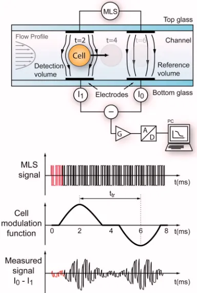
Developments in the field of Lab on a Chip have made impedance analysis of single micron-sized objects such as cells and beads possible. In particular, we and others30–34 have developed methods in performing impedance spectros-copy of single cells at high speed. In this technique, a num-ber of superimposed rf sine signals are used to measure the impedance of single cells flowing through a microchannel. Impedance measurements based on multiple frequency mea-surements can be used to characterize cellular properties, such as size, membrane capacitance, etc. and to distinguish differences in cell subpopulations.35,36 However, there is a need to perform multifrequency analysis in a short time win-dow. Frequency sweep methods are unsuitable because the typical transit time of a cell is of the order of a millisecond. Multiple superimposed frequency excitations require one dedicated rf lock-in demodulator for each frequency, which is clearly impractical. Therefore, one approach is to use a spectrally dense signal such as chirp or MLS共Fig.2兲.

The MLS technique is particularly attractive because of the high computational efficiency of processing and a good

signal-to-noise ratio. The use of MLS in measuring the

im-pulse response of a linear time invariant 共LTI兲 system has

been established for many years and can be traced back to

1960.37,38 One of the advantages of the MLS technique is

that the energy is delivered to the system regularly in time, because the power spectrum of the excitation signal has a homogeneous frequency distribution; it has a quasiflat spec-trum共white noise like兲expect for dc.39

[image:3.612.93.522.55.150.2]

In biological impedance measurements the electrode-electrolyte interface presents a number of problems. The in-terfacial impedance, which is generally capacitive, is in se-ries with the sample and may thus hinder measurements at low frequencies because the interface impedance can be or-ders of magnitude larger than that of the cell suspension. It is also preferable to use a low excitation voltage to reduce any

FIG. 1. Diagram showing the MLS measurement technique. The MLS is generated in software, converted to an analog voltage with a D/A converter, and then applied to the sample. An optional transimpedance amplifier converts the current response to a voltage. The signal is converted to digital with an A/D converter. The digital data stream is then processed with minimal delay by a standard desktop computer.

FIG. 2. Principle of using MLS to measure the complex impedance change due when biological cells pass through a capillary channel. The signal am-plification electronics contains a current to voltage conversion stage and a differential amplifier, gainG= 150. The MLS signal is sent continuously to the sensing electrodes, the passage of a cell imbalances the sensor and the differential current is recorded and processed using a computer.

054301-2 Gawadet al. Rev. Sci. Instrum.78, 054301共2007兲

[image:3.612.340.532.407.692.2]

(4)

method has advantages in that applied voltage is constant and can be set to within the linear regime for the electrodes as well as safe for the cells.

B. Generation of MLS

In this section we describe the generation of the MLS.4,44,45Algorithms for generating the MLS and retriev-ing the system impulse response have been developed by several authors.38,39,46,47The MLS is a pseudorandom binary

sequence共PRBS兲 composed of a sequence of 1 and 0,

gen-erated recursively using a series of digital shift registers with selectedXORfeedback, called taps共Fig.1兲. The length Lof the MLS given byL= 2n_{− 1 with}_n_{denoting the order of the}

sequence and also the number of digital shift registers. The feedback loop is recursively implemented as follows:

an=

冉

兺

i=1

n

ciai

冊

mod共2兲. 共2兲

In Fig.1, the output digital signal comes from registera₁and the new generated digital signal goes to register an, which

depends on the states of all the registers and the correspond-ing feedback coefficientsci. Note that the indexiruns from 1

ton along the shift register from right to left.

The primitive polynomial of the sequence is defined from the feedback coefficientsck,

f共x兲= 1 +

兺

k=1

n

ckxk. 共3兲

In this equation the indexkruns from 1 ton along the shift register from left to right.

With any given initial state of the shift registers共except

all zeros兲an MLS can be generated. A “characteristic” MLS,

also called self-similar, can be generated by selecting appro-priate initial states for the shift register values.48 In practice, the 1 and 0 logical states are often mapped into a negative level and positive level, respectively, to produce a sequence for which the net sum is close to zero.

C. Signal processing

The most important property of any MLS is that, expect for a small dc error, its periodic autocorrelation function

␾nn共l兲is the two valued Kronecker function␦共l兲,39

␾nn共l兲=L+ 1

L ␦共l兲−

1

L, 共4兲

with

dc coupled or not to the measurement circuitry. One way to correct for the dc error is to use a so called perfect periodic autocorrelation signal which can be obtained by selecting appropriate values for the MLS signal instead of +1 and −1,49

Vpositive= 1,

Vnegative=

− 1

1 + 2/

冑

L+ 1. 共6兲

The discrete impulse responseg共l兲 of an LTI system under test can be retrieved from the cross-correlation function be-tween the input and output signals␾ny共l兲 and the autocorre-lation function␾nn共l兲of the input signal.

␾ny共l兲=g共l兲ⴱ␾nn共l兲 ⬵g共l兲ⴱ␦共l兲=g共l兲, 共7兲

where theⴱoperator denotes the periodic discrete linear con-volution. Since convolving any function with the Kronecker delta function equates to the function itself, a direct relation-ship between the impulse response of the system and the cross-correlation function␾ny共l兲is implied.

Cohn and Lempel47demonstrated that the periodic

cross-correlation function can be effectively done using a fast M

transform 共FMT兲 which comprises two permutations and a

fast Hadamard transform共FHT兲. Borish and Angell44showed

that this computation requires only 2.5nlog2共n兲addition

op-erations. In this work, the algorithm was implemented inC

共as a mex file in MATLAB兲. The algorithm structure is

out-lined in Fig.3.

Additional improvements to the SNR are also proposed by these authors. Specifically because the desired signals add coherently while the noise adds incoherently, they suggested

preaveraging a number m of response sequences, which

gives an improvement in the SNR of

冑

m.44Using this noise reduction technique implies that rapid changes in the system impedance are averaged out, which results in a trade off between noise reduction and the ability to measure dynamic changes in time. It is also important to note that the response obtained with this technique is the PIR, which only reduces to the impulse response共IR兲if the system relaxation time is shorter than the generation time of the MLS used.

A fast Fourier transform 共FFT兲is then used to convert

each impulse response to the corresponding transfer function of the system usingFFTW.50The transfer function is used to obtain the impedance of the system. The impulse response is padded with an extra zero in order to obtain an impulse

length of 2n _{before the FFT. The FFT calculation returns a}

complex value spectrum with 2n−1 _{frequency points. The}

highest measured frequency f_max is given by the

Nyquist-Shannon sampling theorem as half of the sampling rate fs.

The frequency resolution is defined as the difference between

(5)

two adjacent measured discrete frequencies. Since the dis-crete frequency points are evenly spaced the minimum fre-quencyfminalso corresponds to the frequency resolutionfres,

fmax=fs/2, 共8兲

f_min=f_res=fs/2n. 共9兲

IV. EXPERIMENT

A. Hardware and implementation

The recent availability of fast processors and

analog-to-digital 共A/D兲 converters has allowed the MLS technique to

be implemented for real-time broadband impedance spec-troscopy. At the time of writing A/D converters with sample rates of 200 megasamples/ s and precisions in the order of 12– 16 bits are commercially available. The MLS, in binary

form, is generated using software written in MATLAB and

then converted to a voltage step sequence of fixed amplitude

and timing using a digital-to-analog 共D/A兲 converter

共NI-6251, National Instruments, USA兲. The MLS response from the device is digitized using an A/D converter on the same board. Both D/A and A/D tasks are started simultaneously with a synchronous clock for the conversions. The hardware has to minimize clock-induced time jittering as this could add a significant white noise source to the recovered spectrum.2

In the present case the sequence has a length of 1023 samples共ordern= 10兲and is generated using a sample rate of 1 MHz, i.e., approximately 1000 times per second. The 1 MHz clock frequency is limited by the data acquisition hardware, and the length of the sequence was a compromise

between resolution and the sequence period共approximately

1 ms兲. For an MLS of order 10, a sampling rate at 1 MHz, and according to Eqs.共8兲and共9兲, the spectrum lies between 976.5625 Hz and 500 kHz. The software performs a number of post processing operations, including optional time filters, event triggering, data plotting, and storage.

B. Test systems

Two test systems were used to evaluate the MLS

method. The first is an RC network, where the measured

results are compared with a model of the system and the MLS sequence. The second test was the measurement of

erythrocytes 共red blood cells兲 flowing in a microfabricated

microfluidic impedance sensing chip.

1. RC network

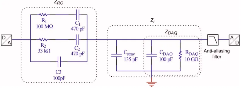
The network shown in Fig. 4was used to test the MLS

[image:5.612.80.535.56.185.2]

system and to validate the behavior against known param-eters. Measurement was performed without current to volt-age conversion, and the input impedance of the data acqui-sition board was used as the sensing resistor and is therefore included in the modeling.

FIG. 3. The digitized MLS response signal is processed using two permutation matrices共SandL兲and a fast Hadamard transform共FHT兲to recover the periodic impulse response. A complex fast Fourier transform共FFT兲is then used to obtain the complex impedance spectrum of the system.

FIG. 4. Schematic of theRCnetwork used to test the MLS system, showing the test networkZRC, the input impedance of the acquisition systemZDAQ, and the stray capacitanceC_stray.

[image:5.612.100.513.581.732.2]

(6)

Because no transimpedance stage is used, the input

im-pedance of the A/D acquisition board ZDAQ influences the

recovered spectrum, as does the A/D antialiasing low pass filters共specified with −3 dB at 1.7 MHz兲. The transfer

func-tionHsysof theRCnetwork measured with the A/D

acquisi-tion board is defined as

Hsys=

Zi

Zi+ZRC

, 共10兲

with

Zi=

ZDAQ 1 +j␻ZDAQCstray

= RDAQ

1 +j␻RDAQ共CDAQ+Cstray兲 ,

共11兲

where Zi comprises the input impedance ZDAQ of the data

acquisition board共NI 6251 DAQ兲and the stray capacitance

Cstray of the coaxial cable. The values for the input imped-ance共taken from the datasheet兲are 10 G⍀resistor共RDAQ兲in parallel with a 100 pF capacitor共CDAQ兲, see Fig.4.

After some algebraic treatment, the impedance ZRC of

theRC network is

ZRC=

A₁共j␻兲2+A₂共j␻兲+ 1

A3共j␻兲3+A4共j␻兲2+A5共j␻兲. 共12兲

The coefficientsAi共i= 1 – 5兲are given in the appendix.

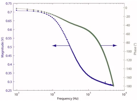
The transfer function of the low pass antialias filterHF

was determined by directly connecting the analog output 共D/A兲to the input共A/D兲with a coaxial cable. Figure5show the measured transfer function spectrum for a 1 V excitation signal. The phase was found to increase to 180° at high fre-quency; this corresponds to a delay of one clock cycle in the impulse response. Since both the D/A and the A/D convert samples simultaneously the impulse peak will not be mea-sured on the first clock but only on the second clock due to nonperfect slew rates and such of the acquisition board am-plifiers. This delay and resulting phase error can be easily compensated in software.

The magnitude and phase of the transfer function of the

RCnetwork system including the filterH_sys_គF are given by

兩HsysគF兩=兩Hsys兩⫻兩HF兩, 共13兲

⬔HsysគF= ⬔Hsys+ ⬔HF, 共14兲

The MLS sequence is generated from the shift register using recursive steps. The output MLS signal, with +1 and −1 levels, is expressed as a time dependent function by the superposition of unit step functionsU0共t兲,

XMLS共t兲=U0共t兲+ 2

兺

i=1

m

共− 1兲i

U0共t−ti兲, 共15兲

where the index i indicates the successive changes in the

MLS signal polarity andtiis the time when each

correspond-ing signal step occurs.

The output response of the system Ysys共s兲 to an MLS

excitationXMLS共s兲can be expressed in thesdomain as:

Ysys共s兲=XMLS共s兲Hsys共s兲. 共16兲

According to the time shift property of the Laplace transform and the superposition principle, the inverse Laplace trans-form of Eq.共16兲is

Ysys共t兲=

冋

Ysys0共t兲+ 2

兺

i=1

m

共− 1兲i

Ysys0共t−ti兲U0共t−ti兲

册

,

共17兲

which is the output response of the system in the continuous time domain corresponding to the MLS excitation. In this equation,Ysys0共t兲=k₁es₁t₊_k

2es2t+k3es3tis the response of the system to a single unit step excitation signalU0共t兲in the time domain.

The same data processing algorithms including the FMT and FFT are applied to the simulated data to retrieve the system transfer function.

Figure6 shows that the data are in excellent agreement

共within 1%兲of the model, indicating that the MLS measure-ment technique can be used to characterize the transfer

[image:6.612.53.294.47.230.2]

func-tion of a passiveRC network.

[image:6.612.316.557.48.226.2]

FIG. 5. The transfer function of the data acquisition board, measured by connecting the input and output with a coaxial cable, showing the influence of the antialias filter and the phase delay at higher frequencies.

FIG. 6. Plot of the magnitude and phase of the transfer function of the network. The model is shown as a solid line and includes the low pass filter. The experimentally measured transfer-function data is plotted as symbols.

(7)

2. Single cell impedance measurement

The sensor chip for single cell impedance analysis is described elsewhere32and is shown in Fig.2. It consists of a capillary channel, 40⫻20␮m2 cross section with two pairs of electrodes placed on opposite sides of the channel. The impedance is measured using a transimpedance amplifier

fol-lowed by a differential amplification stage with gain G

= 150. Because the cells continuously flow between the elec-trodes, the system cannot be considered time invariant.

Erythrocytes were harvested from healthy donors and

suspended in a PBS 共conductivity of 1.6 S m−1_兲 _{prior to}

flowing through the microfluidic channel using a pressure driven flow. In the cell measurements, the impedance is mea-sured differentially and is time varying. The change in im-pedance due to a cell is only between 1% and 5% of the total channel impedance.33The slow共long time period兲variations in impedance due to external parameters were filtered using a moving average offset compensation.

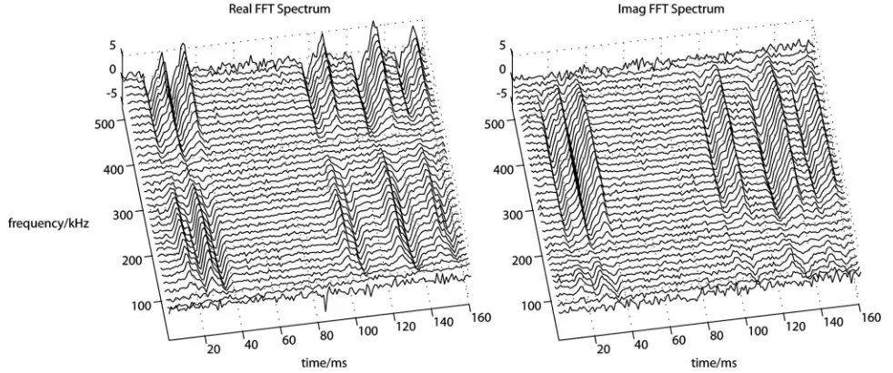
The time averaged spectrogram is therefore flat in the absence of a cell. The MLS data for single cells flowing through the device consists of a spectrogram as shown in

Fig.7. Each cell generates two successive impedance

spec-tral pulses共one positive and one negative兲as it passes over each part of the differential sensor 共see Fig. 2兲. The data show that the spectrum of single cells passing through the detection area in a 20 ms time frame can be clearly resolved 共up to the frequency limit of the acquisition system兲using a MLS having a generation time of a millisecond.

V. DISCUSSION

The measurement of the RC circuit indicates that the

MLS technique can be used to measure the transfer function and therefore the impedance of a共linear time invariant兲 net-work. Preliminary data also show that the technique can also be used to detect the movement of cells through the micro-chip and to measure the low frequency part of the transfer function, up to 500 kHz. In this frequency range, the mea-surement of the cell is limited by the presence of the

electrode-electrolyte interface capacitance共the double layer兲. The data show for the first time that single cell events can be measured across a wide band of frequencies; only measure-ments at two or three simultaneous frequencies have been reported previously.36 The method allows real-time spectro-grams of the transfer function共and by implication the

com-plex impedance兲 of cells passing through a microfluidic

system.

The data show that although the cell measurement sys-tem is not time invariant, this could be less problematic than is usually the case in acoustic measurements. The results indicate that the MLS measurement technique shows prom-ise for high speed single cell analysis. The flexibility of the system means that the signals can be modified in real time to compensate for various deleterious effects such as parasitic elements or the electrode-electrolyte impedance. These ele-ments can be compensated for using techniques borrowed from acoustics, such as filters which proportionally increases the voltage of the low frequency components of the se-quence. The precompensated signal would increase the smaller measured current signal at low frequencies to com-pensate for the interfacial capacitance. Because the system impedance is measured at a high rate, it would be possible to implement a fast-feedback compensation loop which could take into account slow variations in the impedance due to external effects such as temperature changes or changes in flow speed or conductivity.

In this article we have shown that the MLS technique can measure the transfer function of an electrical system and is able to perform fast broadband dielectric spectroscopy. The underlying theory of MLS generation and processing has been presented and a system has been described which

can measure the transfer function of an RC network. The

[image:7.612.61.552.50.255.2]

measured response is in excellent agreement with an analyti-cal model. The MLS technique is relatively easy to imple-ment and can be used to measure the spectrum of a biologi-cal system with a rate and resolution not reported previously. Future work will concentrate on extending the frequency

FIG. 7. Moving averaged spectrogram showing five consecutive red blood cell events as measured using a differential capillary impedance sensor. Although a 512-frequency-point spectrogram is obtained only a subset of the data is presented here for clarity.

(8)

of this work. The work is partly supported by the funding from Life Science Initiative, University of Southampton. Fi-nally one of the authors 共S.G.兲 would like to gratefully ac-knowledge Professor P. Gascoyne, Professor B. Persson, and B. Böhmer for the discussions and suggestions.

APPENDIX

The coefficientsAi共i= 1 – 5兲in Eq.共12兲are given by

A1=R1R2C1C2, A2=R1C1+R2C2,

A3=R1R2C1C2C3,

A₄=R₁C1共C₂+C3兲+R₂C2共C₁+C3兲,

A5=C1+C2+C3.

1_{Y. Ando,}_{Concert Hall Acoustics}_共_{Springer, New York, 1985}_兲_. 2_{J. Vanderkooy, J. Audio Eng. Soc.}_{42, 219}_共₁₉₉₄_兲_.

3_{D. Griesinger, 101st Convention of the Audio Engineering Society, Los} Angeles Convention Center 共1996兲 http://www.aes.org/publications/ preprints/search.cfm.

4_{D. D. Rife and J. Vanderkooy, J. Audio Eng. Soc.}_{37, 419}_共₁₉₈₉_兲_. 5_{M. Weckstrom, E. Kouvalainen, and M. Juusola, Pfluegers Arch.}_{421, 469}

共1992兲.

6_{I. Schneider, Engineering in Medicine and Biology Society, 1996,} Bridg-ing Disciplines for Biomedicine, ProceedBridg-ings of the 18th Annual Interna-tional Conference of the IEEE, October 31–November 3, 1996, Vol. 5, pp. 1934–1935.

7_{L. Rufer, S. Mir, E. Simeu, and C. Domingues, Journal of Electronic} Testing-Theory and Applications21, 233共2005兲共online兲.

8_{N. Xiang and J. M. Sabatier, Proc. SPIE}_{3720, 390}_共₁₉₉₉_兲_.

9_{N. Xiang and J. M. Sabatier, IEEE Trans. Geosci. Remote Sens.}_{1, 292}

共2004兲.

10_{N. Xiang and D. Chu, Proceedings of the ICSP’04, 7th International} Con-ference on Signal Processing, August 31-September 4, 20042004 Vol. 3, pp. 2433–2436.

11_{M. E. H. Amrani, R. M. Dowdeswell, P. A. Payne, and K. C. Persaud,} Sens. Actuators B47, 118共1998兲.

12_{F. Mansfeld, J. Appl. Electrochem.}_{25, 187}_共₁₉₉₅_兲_.

13_{P. L. Bonora, F. Deflorian, and L. Fedrizzi, Electrochim. Acta}_{41, 1073}

共1996兲.

14_{H. Arai, S. Muller, and O. Haas, J. Electrochem. Soc.}_{147, 3584}_共₂₀₀₀_兲_.

共1996兲.

21_{A. Claye, J. E. Fischer, and A. Metrot, Chem. Phys. Lett.}_{330, 61}_共₂₀₀₀_兲_. 22_{J. Z. Bao, C. C. Davis, and R. E. Schmukler, IEEE Trans. Biomed. Eng.}

40, 364共1993兲.

23_{R. Gómez}_{et al.}_{, Biomed. Microdevices}_{3, 201}_共₂₀₀₁_兲_. 24_{E. Katz and I. Willner, Electroanalysis}_{15, 913}_共₂₀₀₃_兲_.

25_{H. P. Schwan, in}_{Physical Techniques in Biological Research}_{, edited by W.} L. Nastuk共Academic, New York, 1963兲, Vol. 6, pp. 323–406.

26_{H. Pauly and H. P. Schwan, Biophys. J.}_{6, 621}_共₁₉₆₆_兲_.

27_{R. A. Hoffman and W. B. Britt, J. Histochem. Cytochem.}_{27, 234}_共₁₉₇₈_兲_. 28_{H. Morgan, T. Sun, D. Holmes, S. Gawad, and N. G. Green, J. Phys. D}_40,

61共2007兲.

29_{M. J. Hutchings and B. C. Blake-Coleman, Meas. Sci. Technol.}_{5, 310}

共1994兲.

30_{U. D. Larsen, G. Blankenstein, and S. Ostergaard, Proceedings of} Trans-ducers 1997, Chicago, USA, 1997共unpublished兲.

31_{N. Xiang and K. Genuit, Characteristic Maximum-Length Sequences for} the Interleaved Sampling Method, ACUSTICA-acta acustica Vol. 82

共1996兲, pp. 905–907.

32_{S. Gawad, L. Schild, and P. Renaud, Lab Chip}_{1, 76}_共₂₀₀₁_兲_.

33_{S. Gawad, K. Cheung, U. Seger, A. Bertsch, and P. Renaud, Lab Chip}_4, 241共2004兲.

34_{D. Holmes, N. G. Green, and E. Morgan, IEEE Eng. Med. Biol. Mag.}_22, 85共2003兲.

35_{K. Asami, T. Yonezawa, H. Wakamatsu, and N. Koyanagi,} Bioelectro-chem. Bioenerg.40, 141共1996兲.

36_{K. Cheung, S. Gawad, and P. Renaud, Cytometry}_{65A, 124}_共₂₀₀₅_兲_. 37_{R. E. Scholfield, Electron Technol.}_{37, 389}_共₁₉₆₀_兲_.

38_{W. D. T. Davis, Control}_{10, 302}_共₁₉₆₆_兲_. 39_{N. Xiang, Signal Process.}_{28, 139}_共₁₉₉₂_兲_.

40_{B. Onaral and H. P. Schwan, Med. Biol. Eng. Comput.}_{21, 210}_共₁₉₈₃_兲_. 41_{H. A. Pohl,}_{Dielectrophoresis}_共_{Cambridge University Press, Cambridge,}

UK, 1978兲.

42_{P. R. C. Gascoyne, X. B. Wang, Y. Huang, and F. F. Becker, IEEE Trans.} Ind. Appl.33, 670共1997兲.

43_{G. Fuhr, H. Glasser, T. Muller, and T. Schnelle, Biochim. Biophys. Acta} 1201, 353共1994兲.

44_{J. Borish and J. B. Angell, J. Audio Eng. Soc.}_{31, 478}_共₁₉₈₃_兲_. 45_{D. V. Sarwate and M. B. Pursley, Proc. IEEE}_{68, 593}_共₁₉₈₀_兲_. 46_{F. J. Macwilliams and N. J. A. Sloane, Proc. IEEE}_{64, 1715}_共₁₉₇₆_兲_. 47_{M. Cohn and A. Lempel, IEEE Trans. Inf. Theory}_{23, 135}_共₁₉₇₇_兲_. 48_{N. Xiang and K. Genuit, Acustica}_{82, 905}_共₁₉₉₆_兲_.

49_{H. D. v. Lüke, Frequenz}_{40, 215}_共₁₉₈₆_兲_.

50_{M. Frigo, Proceedings of the ACM SIGPLAN Conference on} Program-ming Language Design and Implementation 共PLDI兲, Atlanta, Georgia, 1999共www.fftw.org兲.