Development and application of inductively coupled plasma mass spectrometric techniques for the precise measurement of trace elements and lead isotopic compositions in geological materials

(1)

Development and Application of Inductively

Coupled Plasma-Mass Spectrometric

Techniques for the Precise Measurement of

Trace Elements and Lead Isotopic

Compositions in Geological Materials

By

Zongshou Yu (M.Sc.)

UNIVERSITY OF TASMANIA

Submitted in fulfilment of the requirements for the degree of Doctor of Philosophy

University of Tasmania

(2)

DECLARATION OF ORIGINALITY

(3)

STATEMENT OF AUTHORITY OF ACCESS

This thesis may be made available for loan and limited copying in accordance with the Copyright Act 1968

Date: /

J

(i-

1~/

(4)

ABSTRACT

Inductively coupled plasma-mass spectrometry (ICP-MS) is a powerful analytical technique, regarded as one of the most successful in atomic spectrometry, and widely used for measurement of a wide range of trace elements in geological materials. In general, this established technique has the merits of high sensitivity, fast analysis capacities, true multi-element abilities, and a very large dynamic linear concentration range. Sample preparation is also relatively simple.

This study has systematically investigated analytical performance characteristics of a high resolution (HR)-ICP-MS instrument (Finnigan Mat Element, Germany). This instrument has been found to be more sensitive, with less spectral interferences (due to the pre-defined setting of different resolutions) than quadrupole instruments. It has been found that only a single internal standard is sufficient to compensate for the instrumental drift during an analytical sequence. The detection limits for some trace elements studied were found to be as low as pg g-1 levels in solution.

To obtain accurate analytical results using ICP-MS, complete sample dissolution is required. Decomposition techniques for the dissolution of different types of geological materials have been studied. Savillex Teflon beaker HF/HN03 digestion

has been found to be sufficient for the complete dissolution of basaltic samples. High pressure HF/HC104 digestion (PicoTrace® TC-805 digestion system, Bovenden,

(5)

for the measurement of low abundance geological samples, due to the lack of ultra-pure reagents. In general, the microwave digestion method has been found to be unsuitable for the total decomposition of geological materials.

Systematic investigation of chelates between several complexing reagents (citrate, tartrate, EDTA and DTPA) and Zr, Nb, Ta, Hf, Th and U ("high field. strength elements" - HFSE) has shown that DTP A can form stable HFSE complexes in solution. These prevent the hydrolysis of HFSE and hence allow the accurate determination of HFSE in geological materials. A complexing method has been developed, which coupled with an appropriate digestion method and ICP-MS, can lead to the accurate determination of HFSE at different levels (particularly higher than 1 µg g-1 of Nb and Ta) in geological reference materials.

(6)

S contents across the melting range represented. Lead is highly incompatible (close

to La) compared to Zn and Cu, and Cu is close to Ni in being among the most compatible elements in this mantle-melt system. This may indicate that the mantle

sulfide is Cu-bearing pentlandite on a Cu-(Ni-)-bearing monosulfide solid solution. Zinc shows a moderate compatibility level, close to that of V, whereas Mo behaves

similarly to La, and Sb is similar to Ce, both metals being significantly more

incompatible than suggested by Sun and McDonough (1989)

Analytical methods for the precise measurement of lead isotopic compositions using

HR-ICP-MS and the latest quadrupole ICP-MS (HP 4500 plus) have been

successfully developed in this study. Based on a series of measurements of

geological reference materials and lead-bearing samples, the precision (%RSD)

values for 208Pbt2°4Pb, 207Pbt2°4Pb, 206Pbt204Pb, 208Pbt2°6Pb and 207Pb!2°6Pb ranged

from 0.05 to 0.12 for HR-ICP-MS and from 0.06 to 0.15 for quadrupole ICP-MS. By

comparison with lead isotope data obtained by thermal ionisation mass spectrometry

(TIMS), the accuracy of both methods was found to be generally better than 0.20%.

The ICP-MS methods tested here are simple and cost-effective compared to TIMS,

suggesting greater potential for application to geological problems in the future.

Finally, lead isotope ratios in base metal sulfide samples collected from the Lady

Loretta deposit in northern Australia have been successfully measured by the

quadrupole ICP-MS technique. The results are in excellent agreement with the lead

isotope data previously measured by TIMS. The wide variation in the lead isotopic

compositions from the Lady Loretta deposit suggests multiple sources for lead in the

(7)

ACKNOWLEDGEMENTS

This study would not be possible if there were not the financial support provided by the Center of Ore Deposit Research of the University of Tasmania. The author would like to thank the following:

Dr Peter McGoldrick of the Center for Ore Deposit Research, University of Tasmania, for his general supervision, advice and assistance throughout my PhD project.

Associate Professor Anthony J. Crawford of the Center for Ore Deposit research, University of Tasmania, for his guidance, advice and support throughout my study. His support, encouragement and assistance were particularly appreciated at the beginning of this project.

Dr Ashley T. Townsend at the Central Science Laboratory of the University of Tasmania for his technical advice, assistance in using HR-ICP-MS facilities and valuable discussion during this project.

Philip Robinson at the School of Earth Sciences, University of Tasmania, for his assistance in the experimental work and valuable discussion. His support, assistance and encouragement in the quadrupole ICP-MS work are also appreciated.

Professor Ross Large, Drs Marc Norman and Vadim S. Kamenetsky for support and useful discussion.

(8)

LIST OF FIGURES

Figure 2.1. Finnigan MAT Element ICP-mass spectrometer (Bremen,

Germany) in operation at the Central Science Laboratory of

the University of Tasmania ... 15

Figure 2.2. Mean instrumental sensitivity for REE at both LR (low

resolution) (top, R = 300) and MR (medium resolution) (bottom, R =3000) ... 18

Figure 2.3. Mean instrumental sensitivity for trace elements showing

the average instrumental intensity of seven analytical runs ... 19

Figure 2.4. Normalised intensity drift curves for uncorrected intensity

(counts s-1 per ng g-1) drift in a 10-hour analytical run with a 10 ng g-1

calibration standard solution ... .21

Figure 2.5. Normalised intensity drift curves for the 115In corrected

instrumental intensity (counts s-1 per ng g-1/counts s-1 per ng g-1 115In)

drift in a 10-hour analytical run with a 10 ng g-1 calibration standard solution ... 22

Figure 2.6. The precision (%RSD) of the instrumental drift for REE

in a 10-hour analytical sequence. Sector field ICP-mass spectrometer

was operated at medium resolution (R = 3000) ... 23

Figure 2.7. The precision (%RSD) of instrumental drift for trace elements

in a 12-hour analytical sequence. Sector field ICP-mass spectrometer

was operated at low resolution (R = 300) ... 23

Figure 2.8. Correlation of trace element concentrations for the basaltic rock

(14)

Figure 2.9. Correlation of trace elements concentrations for the basaltic rock

reference material-T AF AHI between single and four internal standards ... .40

Figure 2.10. Correlation of trace elements concentrations for the basaltic rock

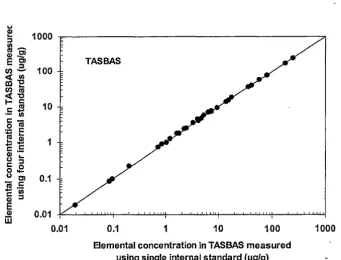
reference material-TASBAS between single and four internal standards ... .41

Figure 2.11. Comparison of analytical results for international rock standard

BHV0-1 using 115In and 185Re as internal standards respectively ... .41

Figure 2.12. Comparison of analytical results for the in-house rock standard

TASBAS using 115In and 185Re as internal standards respectively ... .42

Figure 3.1. PicoTrace® TC-805 Pressure Digestion System: ... 60

Figure 3.2. MLS-1200 MEGA Microwave Digestion System ... 61

Figure 3.3. Comparison between the measured results and reference values

for three basaltic rock standard materials (BHV0-1, T AF AHI and

TASBAS) by Savillex Teflon beaker digestion ... 68

for AC-E. Digestion conditions ... 68

for GSR-1 ... 69

for TASGRAN ... 69

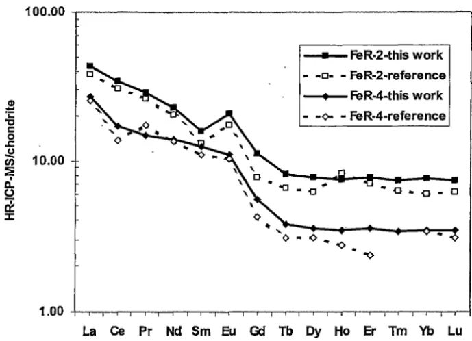
Figure 3.7. Chondrite normalised distribution patterns of REE for FeR-2

(15)

Figure 3.8. Recoveries ofHFSE and REE for GSR-1 and G-2

by HF/HCl04 high pressure digestion ... , ... 81

Figure 3.9. Representative elemental recoveries for GSR-1

using five different digestion methods,. ... 81

Figure 3.10. The recoveries ofHFSE and REE for GSR-1

under various digestion conditions ... 92

Figure 3.11. Comparison ofHR.-ICP-MS results with reference values

for international basalt rock standard BHV0-1 ... 96

Figures 3.12. Comparison ofHR.-ICP-MS results with reference values

for international granite rock standard GSR-1 ... 96

Figures 3.13. Comparison ofHR-ICP-MS results with reference values

for in-house granite rock standard TASGRAN ... 97

Figure 3.14. Comparison ofHR-ICP-MS results with reference values

for magnetite rich rock standard FeR-2 ... 97

Figure 3.15. Chondrite normalised distribution patterns of rare earth

elements for the eight selected geological reference materials

(BHV0-1, TAFAHI, TASBAS, GSR-1, AC-E, TASGRAN, FeR-2

and F eR-4) usin.g lithium tetraborate fusion digestion ... 106

Figure 3.16. Chondrite normalised distribution patterns of rare earth

elements for nine geological reference materials (GSR-1, G-2,

AC-E, TASGRAN, FeR-2, FeR-4, BHV0-1, TAFAHI and TASBAS)

using sodium peroxide sinter decomposition technique ... 116

Figure 4.1. Concentration variations ofHFSE through a 12-hour

(16)

Figure 4.2. Chondrite normalised REE distribution pattern and

comparison with those obtained from the previous reference values

for geological reference material BIR-1 (basalt) ... 138

for geological reference material DTS-1 ( dunite) ... 13 8

for geological reference material DNC-1 (dolerite) ... : ... 139

for geological reference material PCC-1 (peridotite) ... 13-9

for geological reference material UB-N (serpentine) ... 140

Figure 4. 7. Chondrite normalised REE distribution pattern and

for geological reference material T AF AHI (basalt) ... 140

Figure 4.8. Comparison of primitive mantle normalised patterns

for BIR-1, DTS-1 and PCC-1 ... 142

Figure 5.1. A comparison of blank levels (ng g-1) for citrate, tartrate,

EDTA, DTPA and acid blank ... 148

Figure 5.2. Complex stabilities of Zr-citrate, tartrate, EDTA and

DTPA; Nb-citrate, tartrate, EDTA and DTP A; Rf-citrate, tartrate,

(17)

tartrate, EDTA and DTP A and U-citrate, tartrate, EDTA and DTP A

for rock reference material-Mica-Fe (biotite) ... 153

Figure 5.3. Measured concentrations ofHFSE for the geological reference

material - YG-1 by HR-ICP-MS using different chelate reagents ... 156

Figure 5.4. Stability of HFSE- DTPA chelates for the selected geological

reference materials over a period of 5 days after sample dissolution ... 159

Figure 5.5. Stability of HFSE - DTPA chelates for the selected geological

reference materials over a period of 28 days after sample dissolution ... 163

Figure 5.6. Variations of Ta concentrations for GSR-1, Mica-Fe, YG-1

and MA-N over a period of 28 days after sample dissolution ... 166

Figure 5.7. HFSE correlation plot between the measured results and

reference values for the ten selected geological reference materials ... 1 71

Figure 6.1. Comparison of trace element concentrations for glass samples,

60701, G855 and G882b using laser ablation (LA, solid sampling)-,

quadrupole (HP 4500, solution sampling)- and high resolution (HR,

solution sampling)- ICP-MS methods. Results obtained by different

methods were normalised to average values ... 179

Figure 6.2. Comparison of trace element concentrations for glass samples,

40428, G465 and G955b using laser ablation (LA, solid sampling)-, quadrupole (HP 4500, solution sampling)- and high resolution (HR, solution sampling)- ICP-MS methods. Results obtained by different

methods were normalised to average values ... 180

Figure 6.3. Correlation between measured concentrations for elements

with same or very similar incompatibility (Sun and McDonough 1989). Data used for plots were the values of LA-, HP 4500

(18)

Figure 6.4. Correlation between Ti02 concentrations (wt%) measured

by both ICP-MS (including LA-, HP 4500 (quadrupole)- and HR-ICP-MS

methods) and electron microprobe ... 181

Figure 6.5. Relationship between Mg# and major & trace elements

(Ti02, FeO, MgO, V, Cr and Ni) in Macquarie Island primitive glasses

(Group I) and fractionated glasses (Group II, (La!Yb)n = 3-4) ... 186

Figure 6.6. Relationship between (La/Yb )n and Mg# & Fe0%

in Macquarie Island primitive glasses (Group I) and fractionated glasses

(Group II, (La!Yb)n = 3 - 4) ... 187

Figure 6.7. Abundance of major and trace elements vs (La!Yb)n

in Macquarie Island primitive glasses and five fractionated glasses

with (La/Yb )n between 3-4. Trace elements before Dy are in the

incompatibility order proposed by Sun and McDonough (1989) ... 189

Figure 6.8. Plots of Macquarie Island primitive glasses normalised

to most MORB-like sample #47979. Note: Elements are arranged

in the element order of Sun and McDonough (1989) ... 193

Figure 6.9. Plots of the average abundances ofleast, moderately

and most enriched groups normalised to most MO RB-like glass #4 7979 ... 195

Figure 6.10. Mg# vs S, Cu, Zn and Pb in Macquarie Island primitive

glasses and fractionated glasses with (La/Yb )n between 3 and 4 ... 198

Figure 6.11. Most MORB-like glass #47979 normalised plots

of Macquarie Island primitive glasses. a: Plotted using the incompatibility

order proposed by Sun and McDonough (1989) for elements more

incompatible than Yb. b: Organised according to systematically increasing incompatibility during mantle partial melting event responsible

(19)

Figure 7.1. Observed relationship between 208Pb/2°4Pb ratio and

instrumental dead time using 10, 25 and 50 ng g-1 lead solutions ... 206

Figure 7.2. Observed relationship between 207Pb/2°4Pb ratio and instrumental dead time using 10, 25 and 50 ng g-1 lead solutions ... 206

Figure 7.3. Observed relationship between 206Pb!2°4Pb ratio and instrumental dead time using 10, 25 and 50 ng g-1 lead solutions ... 207

Figure 7.4. Relationship between 208Pb/2°4Pb ratio and lead concentrations ... 218

Figure 7.5. Relationship between 207Pb/2°4Pb ratio and lead concentrations ... .218

Figure 7.8. Relationship between 207Pb!2°6Pb ratio and lead concentrations ... .220

Figure 7.9. Corrections of the mercury and tungsten interferences on 206Pb/2°4Pb and 207Pb/2°4Pb using 201Hg and 202Hg isotopes respectively ... 228

Figure 7.10. Correlation oflead isotopic ratio data between sector field ICP-MS and conventional TIMS techniques for 206Pb/2°4Pb ... 233

Figure 7.11. Correlation oflead isotopic ratio data between sector field ICP-MS and conventional TIMS techniques for 207Pb/204Pb ... 233

Figure 7.12. Correlation oflead isotopic ratio data between sector field I CP-MS and conventional TIMS techniques for 208Pb/2°4Pb ... 234

(20)

Figure 7.14. Correlation oflead isotopic ratio data between sector field

ICP-MS and conventional TIMS techniques for 208Pb/2°6Pb ... 235

Figure 8.1. HP 4500 (plus) inductively coupled plasma mass spectrometer (Hewlett Packard, Japan) in operation at the School of Earth Sciences of the University of Tasmania ... 240

Figure 8.2. Relationship between 208Pbi2°4Pb ratio and instrumental dead time using 50, 100 and 200 ng g-1 multi-element solutions ... 242

Figure 8.3. Long-term lead isotope ratio precision using 100 ng g-1 Pb 981 solution. Number of measurements ... 251

Figure 8. 7. Lead isotope precision with concentric nebuliser over a period of two days ... 257

Figure 8.8. Correlation of206Pb/204Pb ratios between the quadrupole-TCP-MS and conventional TIMS techniques ... .261

Figure 8.9. Correlation of207Pb/2°4Pb ratios between the quadrupole-ICP-MS and conventional TIMS techniques ... 262

Figure 8.10. Correlation of208Pbi2°4Pb ratios between the quadrupole-ICP-MS and conventional TIMS techniques ... 262

(21)

Figure 8.12. Correlation of208Pb/2°6Pb ratios between the quadrupole-ICP-MS

and conventional TIMS techniques ... 263

Figure 9.1. Major geological elements and the location of important

Zn-Pb deposits of the northern Australian Proterozoic Zinc Belt

(Large and McGoldrick 1998) ... .266

Figure 9.2. Samples used in this study ... 270

Figure 9.3. Variation of lead isotopic compositions for Lady Loretta

deposit. DDH = diamond ... 272

Figure 9.4 206Pb/204Pb and 207Pb/204Pb ratio plot of four different group

samples from the Lady Loretta deposit. The analytical error shows

two standard deviations using HP 4500 ICP-MS ... 273

Figure 9.5. Lead isotope composition plots for some sediment-hosted

base-metal deposits in the Mount Isa Inlier (modified from Cumming and Richards, 1975). HYC deposit was used as the control

with a geological age of 1640 Ma ... 274

Figure 9.6. Conceptual model of hydrothermal flow for HYC deposit

(from Large et al. 1998; Garven and Bull 1999) ... 276

Figure 9.7. Conceptual model ofhydrothermal flow showing discrete

Pb sources for Lady Loretta deposit (inferred structural setting is from

(22)

LIST OF TABLES

Table 2.1. Typical instrumental settings ... 14

Table 2.2. Memory effects for trace elements at low resolution (R = 300) ... 27

Table 2.3. Memory effects for REE at medium resolution (R = 3000) ... 28

Table 2.4. Example HFSE memory effects associated with the determination

ofBIR-1 ... 28

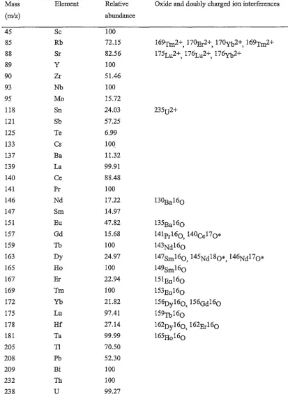
Table 2.5. Oxide, doubly charged ion interferences and relative abundances

of trace elements ... 33

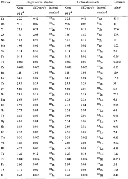
Table 2.6. A comparison of measured trace element concentrations (µg g"1)

for international rock standard BHVO-i' using single and four internal

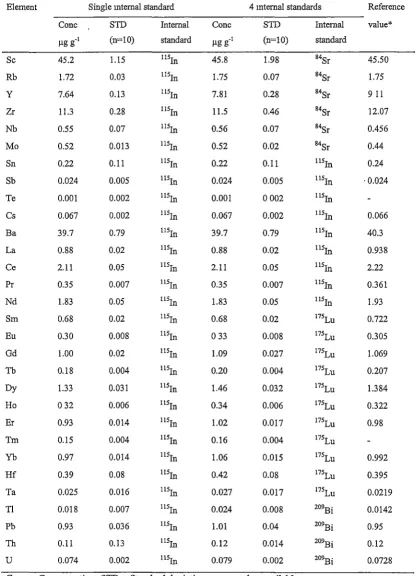
standards ... 37

Table 2.7. A comparison of measured trace element concentrations (µg g-1)

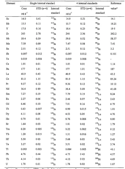
for rock standard TAFAHI using single and four internal standards ... ; ... 38

Table 2.8. A comparison of measured trace element concentrations (µg g"1)

for in-house rock standard TASBAS using single and four internal standards ... 39

Table 2.9. A comparison of REE detection limits between HR-ICP-MS

and some other instrumental techniques ... .44

Table 2.10. Detection and quantitation limits for trace elements ... .45

Table 2.11. Trace element concentrations (µg g"1), precision and reference

(23)

Table 3.1. Geological reference materials studied ... .57

Table 3.2. General physical properties of mineral acids used for sample

digestion and preparation ... 58

Table 3.3. Measured trace element concentrations (µg g-1), precision

and reference values for the three basaltic rock standards: international

standard material BHV0-1, laboratory standard T AF AHI and an in-house

standard TASBAS by Savillex Teflon beaker digestion ... 67

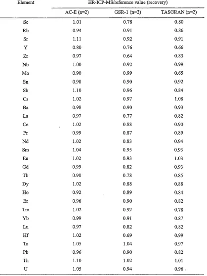
Table 3.4. Comparison between HR-ICP-MS results and reference values

for the granitic rock standards (AC-E, GSR-1 and TASGRAN)

using Savillex Teflon beaker digestion ... 70

Table 3.5. Measured results (µg g-1) for basalt and iron formation reference

materials ... 73

Table 3.6. Measured concentrations (µg g-1) for GSR-1 by HF/HC10JHN0₃

and HF/HC104 high pressure digestion ... 78

Table 3.7. Measured concentrations (µg g-1) for G-2 by HF/HC10JHN0₃

Table 3.8. Measured concentrations (µg g-1) for AC-Eby HF/HCIOJHN0₃

Table 3.9. Measured concentrations (µg g-1), precisions and reference values

for GSR-1 and AC-Eby 3 ml HF/3 ml H2S04 high pressure digestion ... 86

Table 3.10. Measured concentrations (µg g-1), precisions and reference values

for G-2, MA-N, YG-1 and TASGRAN by 3 ml HF/3 ml H2S04 high pressure

(24)

Table 3.11. Measured concentrations (µg g-1), precisions and reference values

for FeR-2, FeR-4, TAFAHI and TASBAS and by 3 ml HF/3 ml H2S04

high pressure digestion ... 88

Table 3.12. Measured concentrations (µg g-1) for GSR-1 using different

HF/H2S04 ratio and digestion time ... 89

Table 3.13. Measured concentrations (µg g-1) for G-2 using different

Table 3.14. Measured concentrations (µg g-1) for AC-E using different

Table 3.15. Comparison of digestion power and pressure among different

microwave digestion works ... 93

Table 3.16. Measured trace and rare earth element concentrations (µg g-1)

and comparison between HR-ICP-MS results and reference values

for eight geological reference materials (BHV0-1, TAFAHI, TASBAS,

GSR-1, AC-E, TASGRAN, FeR-2 and FeR-4) by lithium tetraborate

fusion decomposition ... 102

Table 3.17. Effect of the levels of total dissolved solids (TDS)

on the analytical results for rock reference material TASBAS using lithium

tetraborate fusion decomposition by HR-ICP-MS ... 107

Table 3.18. Measured rare earth element concentrations (µg g-1), precision

and comparison between HR-ICP-MS results and reference values

for nine geological reference materials (GSR-1, G-2, AC-E, TASGRAN, FeR-2,

FeR-4, BHV0-1, TAFAHI and TASBAS) by sodium peroxide sinter digestion ... 110

Table 3.19. Summary of measurable elements by different digestion methods ... 117

(25)

Table 4.2. Procedure detection limits of the low-level analysis of geological

reference materials by HR-ICP-MS and comparisons with those

from previous workers ... 122

Table 4.3. Average measured results (µg g-1), reproducibilities (%RSD) and

comparisons with published values for BIR-1 (basalt) ... , ... 130

Table 4.4. Average measured results (µg g-1), reproducibilities (%RSD) and

comparisons with published values for DTS-1 (dunite) ... · ... 131

comparisons with published values for DNC-1 (dolerite) ... 132

Table 4.6. Average measured results (µg g-1), reproducibilities (%RSD) and

comparisons with published values for PCC-1 (peridotite) ... 133

comparisons with published values for UB-N (serpentine) ... 134

comparisons with published values for T AF AHI (basalt) ... 135

Table 5.1. A list of extra geological reference materials studied ... 145

Table 5.2. Chelate stability constants of high field strength elements ... 146

Table 5.3. Preparation of the 20 mM chelate reagent solutions ... 147

Table 5.4. Blank levels (ng g-1) of citrate, tartrate, EDTA, DTPA and acid

(26)

Table 5.5. Measured results (µg g-1) of HFSE for selected geological

reference materials using DTP A ... 169

Table 6.1. Analyzed elements, isotopes, abundances, internal standards

and resolutions ... ' ... 176

Table 6.2. Major element concentrations (wt%) for "near-primitive"

glass samples (Group I) from Macquarie Island ... 183

Table 6.3. Major element concentrations (wt%) for "fractionated"

glass samples (Group II) from Macquarie Island ... 183

Table 6.4. Trace element concentrations (ppm) for "near-primitive"

glass samples (Group I) from Macquarie Island ... 184

Table 6.5. Trace element concentrations (ppm) for "fractionated"

glass samples (Group II) from Macquarie Island ... 185

Table 7.1. Instrumental signal relative standard deviations (%RSD)

of 2osPbJ204Pb, 201PbJ204Pb, 206pbJ204Pb, 2osPbJ206pb and 201PbJ206Pb

isotope ratios at different passes ... 208

of 2osPbJ204Pb, 201PbJ204Pb, 206PbJ204Pb, 2osPbJ206Pb and 201PbJ206Pb

isotope ratios under a consistent 500 sample data points for each method ... 209

of 2osPbJ204Pb, 201PbJ204Pb, 206PbJ204Pb, 2osPbJ206pb and 201PbJ206Pb

isotope ratios under a total 1000 sample data points for each method ... 209

of 2osPbJ204Pb, 201PbJ204Pb, 206Pb/204Pb, 20sPbJ206Pb and 201Pbf206Pb

(27)

Table 7.5. Instrumental signal relative standard deviations (%RSD)

of 2osPbJ204Pb, 201PbJ204Pb, 206Pb/204Pb, 2osPbf206pb and 201Pbf206Pb

isotope ratios at different sample data points per peak ... 211

Table 7.6. Optimised operating parameters for lead isotopic ratio

measurements ... , ... 212

Table 7.7. Lead isotopic ratio precision data for a standard multi-element

solution (PE-Pb-STD), NIST Pb SRM 981 and a Broken Hill galena (BH2) ... 213

Table 7.8. Instrument mass bias for lead isotope ratios ... 215

Table 7.9. A comparison of lead isotopic ratios of uncorrected, 201Hg

corrected and 202Hg corrected at different mercury concentrations

by sector field ICP-MS with TIMS values ... : ... 222

corrected and 202Hg corrected at different tungsten concentrations

by sector field ICP-MS with TIMS values ... 224

corrected and 202Hg corrected under the co-presence of mercury and tungsten

by sector field ICP-MS with TIMS values ... 226

Table 7 .12. A comparison of lead isotope ratios in NIST Pb RSM 982

and 11 geological samples from different localities in Australia

by sector field ICP-MS and conventional TIMS ... 230

Table 8.1. Typical instrumental settings ... 239

Table 8.2. Relationship between instrumental dead time and lead isotope ratios

(28)

Table 8.3. Instrument signal relative standard deviations (%RSD)

of 2osPbf204Pb 201Pbf2D4pb 206Pbf204pb 2osPbf206Pb and 201Pbf206Pb _, _, _,

in 25, 50 and 100 ng g-1 Pb solutions at different data points per mass ... 243

of 2osPb/204Pb, 201Pbf2D4Pb, 206Pbf204Pb, 2osPbf206Pb and 201Pbf206Pb

in 25 and 50 ng g-1 Pb solutions at different integration time per data point ... 244

of 2osPbf204Pb, 201Pbf204Pb, 206Pbf204Pb, 20sPbf206Pb and 201Pbf206Pb

using 25 and 50 ng

t

1 Pb solutions at different repetitions per mass ... 246

Table 8.6. Optimised instrument operating parameters for the measurement

of Pb isotope ratios using HP 4500 ICP mass spectrometer ... 246

Table 8.7. Lead isotope ratio precision (short-term) and theoretical

precision using BH2 digest. Lead ratios were analysed at Pb concentrations

of 50, 100 and 200 ng g-1 ....•.•...••••...•••••••.••..•...•....•...• 248

Table 8.8. Lead isotope ratio precision (short-term) and theoretical

precision using NIST Pb 981. Lead ratios were analysed at Pb concentrations

of 50, 100 and 200 ng g-1 •...•..•....•...•..•.•..••.•.••...•.•.••..•... 249

Table 8.9. Lead isotope ratio precision (short-term) and theoretical

precision using multi-element standard solution. Lead ratios were analysed

at Pb concentrations of 50, 100 and 200 ng g-1 ...•... 249

Table 8.10. Long-term lead isotope ratio precision (%RSD)

using 100 ng g-1 BH2 digest. ... 252

Table 8.11. Lead isotope precision (%RSD) with concentric nebuliser

(29)

'Table 8.12. A comparison of lead isotope ratios in NIST Pb RSM 982

and 11 geological samples from different localities in Australia

, by quadrupole-ICP-MS, HR-ICP-MS and TIMS ... 259

Table 9.1. Comparison of geological ages (U-Pb zircon ages)

and Terrain Specific Control Model ages ... 268

Table 9.2. Lead isotopic compositions for the Lady Loretta deposit ... 271

(30)

Chapter 1 INTRODUCTION

Understanding the behaviour of trace elements over a wide range of temperatures, pressures and environments applicable to the Earth has played an important role in formulating models of a variety of geological processes. These processes include magmatic and metamorphic differentiation, mantle and crustal anatexis as well as ore-formation. Evaluating models for these processes requires accurate and precise measurements of trace element abundances in rocks and minerals, a major focus of analytical geochemistry for many decades.

Gray (1989) conducted a survey of available and emerging spectrometric techniques suitable for multi-element analysis and concluded that atomic mass spectrometry (MS) was the only potential technique which could offer· the combination of simple spectra, adequate resolution and low detection limits that was desirable for multi trace element determination in complex matrices. In order to improve the precision, sensitivity, detection limit and increase dynamic range of the conventional MS technique, inductively coupled plasma-mass spectrometry (ICP-MS) was initially developed from the work of Gray (1975), who demonstrated that good detection limits can be obtained and isotope ratios can be determined when a solution is introduced into a d. c. plasma (DCP) at atmospheric pressure and the ions formed are extracted into a mass spectrometer.

At present, although ICP-MS has become a standard and routine analytical technique for the analysis of trace elements in geological samples (e.g. Jenner et al. 1990; Eggins et al. 1997), quality analysis of geological materials presents a particularly challenge for ICP-MS due to:

(31)

(b) limitation in low abundance analy,,sis due to the low sensitivity of the older generations of quadrupole instruments and other problems such as memory effects (particularly for low abundance Nb and Ta analyses);

( c) the hydrolysing tendency of high field strength elements (HFSE: Nb, Ta, Zr, Hf, Th and U) in aqueous solutions (e.g. Perrin 1964; Heslop and Jones 1976; Miinker 1998).

Furthermore, attempts were made to analyse lead isotope ratios using old generations of quadrupole instruments to reduce the high cost of lead isotope ratio measurement in geological materials using the conventional thermal ionisation mass spectrometry (TIMS) (Smith et al. 1984; Date and Cheung 1987; Longerich et al. 1992). However, those instruments were specifically designed for the rapid scanning of relatively large mass ranges and sensitivities were relatively low. Therefore, the precision and accuracy of lead isotope ratio data were limited by counting statistics.

In order to overcome and better understand these limitations, this thesis presents a systematic investigation of dissolution techniques for different types of geological materials, analytical methods for the reliable measurement of trace elements at low abundance, and a new technique for measuring lead isotope ratios using a high resolution (HR)-ICP-MS and current generation quadrupole ICP-MS.

1.1 Inductively Coupled Plasma-Mass Spectrometry

(32)

British Geological Survey (headed by Date) and VG Instruments (Horlick et al. 1987).

The first ICP-MS system certainly showed promise of very high sensitivity, giving essentially zero background levels between mass peaks and signals of between 104 and 105 counts per second (cps) for fully ionised mono-isotopic elements such as Co at a concentration in solution of 1 µg mr1 (Gray 1989). Haulk et al. (1980) studied inductively coupled argon plasma (ICAP) as an ion source for mass spectrometric determination of trace elements and found that the positive ion mass spectrum obtained during nebulization of a typical solvent (1 % _{HN03 in H20) consisted}

mainly of Arir, Ar+, H30+, NO+, 02+, HO+, Ar1+, Ar1H+ and Af2+, and the mass spectra of the trace elements investigated consisted mainly of singly charged monatomic

(Ml

or oxide (MOl ions in the correct relative isotopic abundances. Based on the elements studied, Houlk et al. (1980) found that working range generally covered nearly 4 orders of magnitude with detection limits of 0.002-0.06 µg m1-1. As summarised by Jarvis and Jarvis (1992), the main advantages ofICP-MS for the analysis of geological materials include:

1. rapid simultaneous multi-element measurement;

2. superior sensitivity and detection limits, particularly for heavy elements; 3. wide linear dynamic range of at least 6 orders of magnitude;

4. simple spectra and low background even for complex matrices; 5. adequate precision, reproducibility and good accuracy;

6. rapid isotope ratio capacity, enabling stable-isotope tracer studies and the use of isotope-dilution techniques for optimum precision and accuracy;

7. excellent performance for "difficult" elements (such as rare earth and high field strength elements).

(33)

solution concentrations in excess of 10 µg m.r1, and the use oflarge apertures in the continuum mode, which should greatly increase the upper concentration limit of the system, was initially prevented by the formation of the "pinch" discharge in the aperture mouth caused by compression of the electron population of the plasma gas. Date and Gray (1983a and 1983b) found that, by regulating the pressure immediately behind the sampling aperture, it was possible to suppress the discharge and achieve controlled expansion of the plasma gas into the vacuum system. By sampling in this way with ICP-MS, the sampled gas was no longer cooled immediately in front of the aperture, and there was little salt condensation around the aperture rim for salt concentrations up to 1 OOO µg mr1• Furthermore, because the ionisation equilibrium

in the sampled plasma corresponded more closely to plasma rather the boundary layer temperatures, ionisation suppression was greatly reduced.

In the meantime, Gray and Date (1983) studied inductively coupled plasma source mass spectrometry using continuum flow ion extraction. Detailed operating characteristics and performance of the continuum flow ion extraction system were investigated in the work. Houk et al. (1983) investigated mass spectra and ionisation temperatures in an argon-nitrogen inductively coupled plasma. Positive ions were extracted from the axial channel of an inductively coupled plasma (ICP) in which the out gas flow was Ar, N2 or a mixture of Ar and N2 in their work. They found that

Ar2+, 02+ and ArH+ reacted with N-containing species in the plasma and/or during

the ion extraction process and ionisation temperatures measured from the ratio Cd+

It

were 5750-6700 K for a N2 outer flow ICP at a forward power of 1.2 kW.

(34)

ICP mass spectrometers equipped with a double-focusing magnetic sector mass spectrometer, instead of a quadrupole filter, have also been commercially available since 1989. These instruments are also referred to as HR-ICP mass spectrometers due to their ability to resolve isotopes from molecular ions, which cannot be done using quadrupole instruments. The heart of a double-focusing instrument is a magnetic sector field. If ions that have uniform energy but different mass are injected perpendicular to a magnetic sector field, they pass the field on a circular trajectory because of Lorentz force. The radius of the trajectory depends on the mass of the ion, leading to a mass dispersion.

However, it was not until 1996 that precise measurement of isotope ratios with a double-focusing magnetic sector ICP mass spectrometer was reported by Vanhaecke et al. (1996). It was also found that double-focusing magnetic sector ICP-MS, operated under low resolution conditions, yielded a remarkable improvement in isotope ratio precision relative to quadrupole-based ICP-MS. Vanhaecke et al. (1997) also studied the applicability of HR-ICP-MS for the accurate and precise measurements of isotope ratios of which at least one of the isotopes involved was spectrally interfered when measrired at low resolution (using copper as a typical example). Their study showed that HR-ICP-MS, operated at a resolution setting of 3000, could be successfully used to determine the natural 63Cu/65Cu ratio in both an Antarctic sediment sample and a human serum reference material, even though the isotopes involved severely isobarically interfered with each other at low resolution.

(35)

1.2 Decomposition of Geological Samples

Sample decomposition is a fundamental and critical stage in the process of geochemical sample analysis. It is often the limiting factor to sample throughput, which is particularly true with the recent application of the fast and modem multi-element measurement instrumentation, such as ICP-AES and more recently ICP-MS.

Many digestion methods have been used for the decomposition of geological samples. These include open and closed vessel acid digestion methods (Moselhy et al. 1978; McQuaker et al. 1979; Lechler et al. 1980; Church 1981; Uchida et al. 1980; Lechler et al. 1980; McLaren et al. 1981; Hee and Boyle 1988; Karstensen and Lund 1989; Dulski 1994; Mfinker 1998; Liang et al. 2000), microwave dissolution (Lamothe et al. 1986; Borman 1988; Kingston and Jassie 1988; Mathes 1988; Matusiewicz and Sturgeon 1989; Kemp and Brown 1990; Ncnter et al. 1990; Totland et al. 1995; Yoshida et al. 1996), Na20 2 sintering (Robinson et al. 1986; Potts 1987; Chao and Sanzolone 1992), and fusions with a~ali fluxes such as LiB02, Li2B407,

Na20 2 etc. (Burman et al. 1978; Bankston et al. 1979; Walsh and Howie 1980; Brenner et al. 1980; Norman et al. 1989).

Despite this multitude of techniques, in practical ICP-MS analysis, caution must be taken when adapting them for multi-element determination since some of the digestion procedures were only developed for measurement of one or several elements. In fact, the solution chemistry involved in many dissolution procedures is poorly understood and refinements and understanding of these techniques have not kept pace with the rapid development in modem analytical instrumentation (Totland et al. 1992).

Hence, one of the main aims of this thesis is a systematic investigation on the decomposition technique for a wide range of geological reference materials with a view to achieving complete dissolution.

(36)

Lithophile trace elements can be present at very low levels (~ng g-1) in some rocks,

particularly ultramafic rocks (such as peridotite and dunite), and the limited instrumental sensitivity generally associated with older generations of quadrupole ICP-MS means that their quantitative measurement often becomes problematic and complicated. For instance, Makishima and Nakamura (1997) used flow injection ICP-MS to measure Rb, Sr, Y, Cs, Ba, REE, Pb, Th and U at ng g-1 levels in silicate

samples.

The determination of high field strength elements (HFSE) in solution is particularly

difficult because:

1. HFSE are often contained in refractory minerals that are resistant to acid attack, and they also have a tendency to polymerise or hydrolyse in aqueous

solution.

2. Memory effect is one of the most important problems associated with the

accurate measurement of HFSE. As reported by McGinnis et al. (1997), the

HFSE generally exhibit a "sticky" nature in which they may adhere to the surfaces of the sample introduction system, allowing for the possibility of

remobilisation by trace amounts of hydrofluoric acid (HF) present in the rock solution.

3. Sample dissolution often needs to be carried out in strict "clean-room"

laboratory conditions when analysing low levels (Ionov et al. 1992).

For the purpose of low level analysis, this thesis presents an application of HR-ICP-MS techniques in conjunction with high pressure HC104/HF digestion by developing

a reliable analytical method for low abundance analysis. The technique is tested on

six selected low abundance reference materials (including BIR-1, DTS-1, PCC-1

etc.).

1.4 Measurement of Lead Isotope Ratios

The study of the lead isotopic composition of rocks and minerals began in the early

(37)

instrumentation, notably TIMS, lead isotopic analysis became widely applied. The widespread use of lead isotopes in geological studies began in the 1950s & 60s (Cannon et al. 1961 and Rankama 1963) and it has received increasing attention since then (Doe and Stacey 1974; Gulson and Mizon 1979; Smith et al. 1984; Gulson 1986; Marcoux and Moelo 1991; Le Guen et al. 1992; Arribas and Tosdal 1994;

Foley and Ayuso 1994; Arias et al. 1996; Childe 1996).

Currently, TIMS is the technique of choice for all types of geological lead isotope·

measurements in order to achieve satisfactory accuracy and precision. However, the relative high cost of the instrumentation and complicated chemical pre-treatment of

geological samples, usually involving ion exchange separation due to serious isobaric

interferences (Potts 1987), have imposed serious limitations on the widespread

application of Pb isotope techniques to routine geological exploration programs.

The ability of quadrupole ICP-MS to measure lead isotopic ratios was initially

demonstrated by Smith et al. (1984), followed by Date and Cheung (1987) and Longerich et al. (1992). However, quadrupole ICP-MS instruments are specifically

designed for the scanning of relatively large mass ranges, and such are inherently less

stable than magnetic sector ICP-MS and cannot achieve the accuracy and precision needed for isotope ratio analysis.

After carefully considering all possible causes of instrumental bias, Begley' and Sharp

(1997) recently undertook a rigorous investigation of lead isotopic ratios using a

quadrupole ICP-MS instrument. The precision obtained from the analysis of NIST

Standard Reference Material (SRM) 981 Natural Lead ranged from 0.04 to 0.12%

(depending on the ratio studied). This accuracy and precision has been until now the best presented from a quadrupole ICP-MS instrument. However, despite the use of

high Pb concentration (1000 ng g-1) in testing solutions, Begley and Sharp (1997)

were still unable to report the ratio data of 207Pb/2°4Pb and 208Pb/2°4Pb using an early model quadrupole ICP-MS instrument (VG Micromass Model 12-12S).

Sector field ICP-MS overcomes many of the inherent problems exhibited by quadrupole instruments, and is becoming more used for the precise measurement of

(38)

it has been applied in a variety of fields such as environmental and biological analysis, and the monitoring ofradionuclides (Becker and Dietze 1997). However, to date little has been made of the sector field ICP-MS for measuring lead isotopic ratios in geological samples (Shuttleworth et al. 1997).

In this thesis, the feasibility of precisely measuring lead isotope ratios in geological materials (mainly sulfides) using sector field ICP-MS (Finnigan MAT Element) and a recent quadrupole ICP-MS (HP 4500 plus) is systematically investigated. In addition, as a case study, a group of selected sulfides from the Lady Loretta deposit is measured for lead isotopic compositions using the HP 4500 ICP-MS.

1.5 Measurement of HFSE

HFSE play an important role in understanding and interpreting petrogenetic processes (Sun and McDonough 1889; Rollinson 1993). However, due to their tendency to hydrolyse in aqueous solutions, reliable measurement of HFSE has been a challenge (e.g. Perrin 1964; Heslop and Jones 1976; Milnker 1998).

(39)

measured concentrations of Zr, Nb, Hf and Ta were found to be lower than those

provided by isotope dilution-spark source mass spectrometry (ID-SSMS) and instrument neutron activation analysis (INAA). Low results for Zr, Nb, U Th were also noted with the analysis of Japanese rock reference samples (including basalt, granodiorite, rhyolite, gabbro apd andesite) by ICP-MS (Yoshida et al. 1996). Preliminary work for this thesis, despite the use ofH2S04/HF high pressure digestion

method and fresh solution determinations, yielded low HFSE recoveries for high

HFSE abundance rock standards, due to the hydrolysis of HFSE in aqueous

solutions. For instance, recoveries for Nb, Hf and Ta were found to less than 50% of

published values (Govindaraju 1994). Low Ta recovery was also found for samples containing more than 1 µg g-1 in solid, such as AC-E, GSR-1, YG-1, TASBAS and

TASGRAN.

This study reports the investigation of a range of chelating reagents to prevent or

minimise hydrolysis of HFSE in aqueous solutions in order to obtain reliable

analytical data for HFSE in geological materials.

1.6 Scope of this Study

I

In summary, the major objectives of this project have been to evaluate and optimise a

variety of geoanalytical techniques based on ICP-MS analysis of multi trace elements

and lead isotope ratios in geological samples. Specifically, I report herein:

• an investigation of the performance characteristics ofHR-ICP-MS associated with the measurement of multi trace elements in geological samples.

• optimized decomposition techniques for the analysis of geological samples

(mainly silicates such as basalt, granite, dunite, peridotite, dolerite, serpentine etc.) byICP-MS.

(40)

• an investigation of the use of complexing reagents ,to improve the accuracy of HFSE measurements in geological materials using ICP-MS.

• development of a method for the accurate and precise measurement of lead isotope

ratios in geological samples using HR-ICP-MS, and study the interference and correction of Hg and W on the measurement of Pb isotope ratios.

• development of a method for the accurate and precise determination of lead

isotopic compositions in geological samples using a modem quadrupole ICP-MS.

Application of these techniques is demonstrated via two case studies:

• an evaluation of the relative compatibility/incompatibility of a range of trace elements, especially the rarely analyzed (in basaltic rocks) Mo, Sn and Sb in a

suite of basaltic glasses from Macquarie Island in the Southern Ocean.

• a Pb isotope investigation of a representative suite of sulfides from the Lady

(41)

Chapter 2 PERFORMANCE CHARACTERISTICS OF

SECCTOR FIELD ICP-MS FOR THE

DETERMINATION OF TRACE ELEMENTS

IN

GEOLOGICAL MATERIALS

2.1 Introduction

Although ICP-MS has its origin in the 1970s, in comparison with some other analytical techniques (such as INAA, XRF and ICP-AES etc.), it is still a relatively

new technique for high precision trace element analysis in geological samples. In the

past, the analytical performance of the quadrupole ICP-mass spectrometer has been studied and the quadrupole ICP-MS has been successfully applied to the analysis of

trace elements in geological samples by several workers (e.g. Riddle et al. 1988; Garbe-Schonberg 1993; Hollocher and Ruiz 1995; Eggins et al. 1997). By contrast,

little has been reported on the analytical performance, and applications to the

analysis of trace elements in geological samples by sector field ICP-MS. In this

chapter, comprehensive performance characteristics of a sector field ICP-MS

(Finnigan MAT Element ICP-mass spectrometer with a double-focusing magnetic

sector mass analyser of reversed Nier-Johnson geometry) for determination of trace elements in geological materials will be discussed.

2.2 Experimental

2.2.1 Reagents and Standards

HF (50% w/w Analar, AR grade), HCl (33% w/w BDH, AR grade) and HN03 (70%

w/w BDH, AR grade) were all used in this study for sample decomposition. HCI and

HN03 were further doubly distilled in a sub-boiling quartz distillation system before

(42)

ultra-pure HC104 (70% w/w ARISTAR®, BDH Chemicals) was also used. Ultra-pure

water(~ 16.7MQ) used in the study was first distilled with a glass distillation system and then further purified with a MODULAB Water Purification System (Continental Water System Corporation, Melbourne, Australia).

External calibration standards were prepared by gravimetric serial dilution from 100

µg mr1 multi-element standards (QCD Analyst, USA). The standard solutions were prepared at the beginning of each analytical sequence with doubly distilled water and

2%HN03.

Indium and lutetium standard solutions (1000 ± 3 µg mr1 in 2% HN03, High-Purity

Standards (South Carolina, USA)) were diluted to working concentration in 2%

HN03 before use as internal standards for ICP-MS analysis. An 84Sr isotope solution (83.2% 84Sr, provided by the University of Adelaide), Re and Bi (high purity

standard from Spex Chemical & Sample Preparation, USA) were additionally used as internal standards for comparison purposes.

2.2.2 Instrumentation

A Finnigan MAT Element ICP-mass spectrometer (Bremen, Germany) was used in

this study (Figure 2.1). The instrument is in operation at the Central Science Laboratory of the University of Tasmania, and is equipped with a compact

double-focusing magnetic sector mass spectrometer ofreversed Nier-Johnson geometry. The

mass range of the double-focusing magnetic sector field analyser extends from 5 to

260 atomic mass units. Pre-defined resolution settings (ml Lilli at 10% valley

definition) of 300 (low), 3000 (medium) and 7500 (high) allow the operating

resolution to be adjusted, depending mainly on the analytical matrices met. As a

result, this type of instrumentation is often referred to as sector field or high-resolution (HR) ICP-MS. Both "sector field ICP-MS" and "HR-ICP-MS" are used throughout this thesis. In this investigation, isotopes of interest were measured using electric scanning, with the magnet held at fixed mass. Instrument tuning and

optimisation were performed daily using a 10 ng g-1 multi-element solution containing the elements of interest. In general, instrument parameters were adjusted

(43)

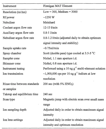
study are summarised in Table 2.1. Further details regarding this instrument have

been reported elsewhere (Moens et al. 1994; Townsend et al. 1998; Robinson et al.

[image:43.572.89.516.176.698.2]

1999; Yu et al. 2000).

Table 2.1. Typical instrumental settings for the Finnigan MAT Element

Instrument

Resolution (m/&n)

Rfpowe~

Nebuliser

Coolant argon flow rate Auxiliary argon flow rate

Nebuliser argon flow rate

Sample uptake rate

Spray chamber Sampler cone

Skimmer cone Instrument tuning

Ion transmission

Finnigan MAT Element

Low= 300, Medium = 3000

~1250W

Meinhard 12-13 l/min

0.8-11/min

0.8-1.21/min (adjusted daily to obtain optimum

signal intensity and stability)

~o. 75ml/min

Scott (double pass) type cooled at 3.5-5 °C Nickel, 1.1 mm aperture i.d.

Nickel, 0.8 mm aperture i.d.

Performed using a 10 ng g-1 multi-element solution

~1,000,000 cps per 10 ng g-1 indium at low

-resolution

Rinse time between standards 200 sec (with 5% HN03) or samples

Takeup and equilibrium time 240 sec

Scan type Magnetic jump with electric scan over small mass

range

Ion sampling depth Adjusted daily in order to obtain maximum signal intensity

(44)

(45)

2.3 Instrumental Sensitivity

Instrumental sensitivity (counts s-1 per ng g-1) depends on the efficiency of sample

jntroduction, ion transmission through the plasma - vacuum interface and lens stack, instrumental tuning, and the performance of the detector in ICP-MS analysis.

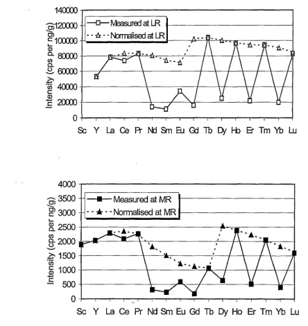
The mean sensitivities (counts s-1 per ng g-1) for REE at low resolution (R = 300) and

medium resolution (R = 3000) are given in Figure 2.2. The mean instrumental

sensitivities at low resolution are the average intensity values of 7 separate

measurements during a 12-hour analytical run. Figure 2.2 (top) shows that

HR-ICP-MS is a very sensitive analytical technique. The intensity range for REE is between 103925 and 52989 counts s-1 per ng g-1 from the intensity normalised to 100%

isotopic abundance. The measured instrumental intensities for REE are in the range of 16018 to 103925 counts s-1 per ng g-1• G~dolinium shows the lowest instrumental

intensity (16018 counts s-1 per ng g-1) simply due to the lowest isotope abundance of

15.68% for the isotope 157Gd. On the other hand, the normalised intensities for REE are in the range of 52989 to 103925 counts s-1 per ng g-1• Terbium has the maximum

normalised intensity, whereas Y has the minimum normalised intensity. The

saw-toothed shape for the measured intensity curve is largely produced by the difference in isotopic abundance. For' instance, the intensities for 139La, 141Pr, 159Tb, 165Ho,

169

Tm and 175Lu with 100% or close to 100% isotopic abundance are clearly higher

than those (ie. 14°Ce 88.50%, 146Nd 17.22%, 147Sm 14.97%, 151Eu 47.80%, 157Gd

15.68, 163Dy 24.97%, 167Er 22.94% and 172Yb 21.82%) with lower isotopic

abundance. In addition, the difference in the ionisation energy may also be

responsible in part for the saw-toothed shape for the measured intensity curve (Jarvis et al. 1992).

Due to strong interferences by silicon oxides (such as 29Si160 and 28Si1601H, also see Finnigan MAT Element ICP-MS Interference Tabk for more information), Sc is

generally determined at medium resolution (R = 3000). In practical HR-ICP-MS analysis, in order to avoid severe interferences from a complicated matrix, Y and REE are also determined at medium resolution. Hence, the instrument intensities for Sc, Y and REE are also described herein. Normally, the instrumental intensities of

(46)

The mean instrumental sensitivities at medium resolution were the average intensity values of 6 separate measurements during a 10-hour analytical sequence. Figure 2.2 (bottom) shows that HR-ICP-MS is st_ill a very sensitive analytical technique, even at medium resolution. The measure intensity is between 176 and 2384 counts s-1 per ng g-1

. Again Gd gave the lowest measured intensity value mainly due its low isotope

abundance. The intensity range for REE is between 2535 and 1122 counts s-1 per ng g-1 from the intensify normalised to 100% isotopic abundance. It also can be found that Dy has the maximum intensity, and Tb has the lowest intensity from the intensity normalised to 100% isotopic abundance. Similarly, the saw-toothed shape for the measured intensity curve is mainly caused by the difference in isotopic abundance and ionisation energy of individual isotopes.

The mean sensitivities (counts s-1 per ng g-1) for trace elements at low resolution (R

'

= 300) during a 10-hour analytical run are given in Figure 2.3. The intensity range

for trace elements is from 98748 to 12318 counts s-1 per ng g-1 from the intensity normalised to 100% isotopic abundance, which is much higher than the normal quadrupole ICP-MS (Begley and Sharp 1997). Uranium has the maximum intensity, and Te has the minimum intensity from the intensity normalised to 100% isotopic abundance. The saw-toothed shape for the measured intensity' curve is also caused by the difference in isotopic abundance and ionisation energy of individual isotopes. The isotopic abundances of trace elements used in this work are 72.15% for 85Rb, 82.56% for 88Sr, 51.46% for 90Zr, 100% for 93Nb, 15.72% for 95Mo, 24.03% for

118

Sn, 57.25% for 121Sb, 6.99% for 125Te, 100% for 133Cs, 11.32% for 137Ba, 27.14% for 178Hf, 99.99% for 18Ta, 70.5% for 205Tl, 52.3% for 208Pb, 100% for 209Bi, 100% for 232Th and 99.27% for 238U. As clearly seen in Figure 2.3, Mo, Te and Ba gave very low values of the measured instrumental intensities mainly due to their low isotope abundances.

Comparison between sector field and quadrupole ICP-MS methods: Sector field

(47)

115In, whereas the attainable sensitivity for a quadrupole instrument has been reported as (2-5) x 104 counts s-1 per ng g-1 115In (Eggins et al. 1997).

140CKJo-.-~~~~~~~~~~~~~~~~~~~~

-12CXXJ0

-0--Mmured at LR

~

g>

1 CXXXJO - --t:x • • l\brrralised at LR

I

-Q)

c.. 8CXXJO-t---l!i:.:::::~7'"""'('-=--'-:U:-.--;:-:.---;----r-t---t-t---ir---t---w

[ • -h.- -

tl

~ 6CXX)()+--~,__ _ _ _ _ _ _ _ _ _ _ _ , _ - - l - - f - - l - - - f - - - + - - - - l - l

~ 4CXX)()+---~-~----1---~-~1--~-t-1---\-f----\t----l---I

c Q)

c

2CXXJ0-1---~---\---=---u---4~---l

O+--,-~.,...--.----,~-.----..~-.---r-~.,...--.----,~-.---.~-.----1

Sc Y La

Ce

Pr

l\k:f

Sm

Eu

Q:I Tb Dy

1-b

Er

Tm Yb Lu

4000-.-~~~~~~~~~~~~~~~---0)

3500

• Measured at MR

-

g>

3000

--* --

Normalised at MR ____________ _,

I

-~

2500

-1---c---~---1

fr

2000

.i.-:::...---\---'-:---____!.---J-l,.---a.,.--,---1

--

~ 1500-+---+---'--l-~--l---\---'ll'

·u;

a5

1 OOO -1---\---~-~-1----r-1----\---1--1

+-'

c 500+-~~~~~-\-~--~---/-~---=-~-tm-~~---I

0+----.-~.,.--,-~.,...--..,..-~~-.---..~...,.._--....~..,-...,...~...-... ---1

[image:47.572.59.503.117.587.2]

Sc Y La

Ce

Pr Nd Sm Eu Gd Tb

Dy

Ho Er Tm Yb Lu

Figure 2.2. Mean instrumental sensitivity for REE at both LR (low resolution) (top, R = 300) and MR (medium resolution) (bottom, R =3000). The testing solutions

were in 2% HN0_{3. The measured shows the instrumental intensity at the analytical}

masses (45Sc, 89y, 139La, 140Ce, 141Pr, 146Nd, 147Sm, 1s1Eu, 1s1Gd, 1s9Tb, 163Dy, 165Ho, 167_Er,169_Tm,172_{Yb and}175_{Lu). The normalised plots show the intensity normalised}

(48)

100000

90000

•

Maasured

...

-

80000

. . * . .

Norrralised

~

O"l ₇₀₀₀₀

c::

...

Q)

60000

0..

en

0.. ₅₀₀₀₀

()

...

~ 40000

·u;

c::

30000

2

E

20000

10000

Resolution= 300 0

Rb Sr Zr Nb Ml Sn Sb Te Cs Ba Hf Ta 11 Pb Bi Th u

Figure 2.3. Mean instrumental sensitivity for trace elements showing the average

instrumental intensity of seven analytical runs. The testing solutions were in 2% HN03. Masses used in this investigation are 85Rb, 88Sr, 91Zr, 93Nb, 95Mo, 118Sn, 121Sb 12sTe 133Cs 137Ba 178Hf is1Ta 2osTl 20sPb 209Bi 232Th and 23sU

' ' ' ' '

' ' ' '

.

2.4 Instrumental Drift

One of the p1incipal limitations on the accuracy of the ICP-MS technique is the drift

of the instrumental response relative to the calibration standard during the course of

an analytical sequence. Instrumental drift is often a complicated function of mass and

can 'be the single most important factor in determining the accuracy of an ICP-MS

analysis (Norman 1997). The instrumental drift expressed as the maximum deviation

of a single measurement on the calibration standard from the average is usually less

than 20% within one shift (8-12 hour) run (Jackson et al. 1990). With a quadrupole ICP-MS method, several internal standards are generally spiked into sample

solutions to correct the instrumental drift (Jackson et al. 1990; Jenner et al. 1990; Eggins et al. 1997). For instance, Jem1er et al. (1990) used three mass-dependent drift correction factors to correct the instrumental drift. A light mass correction factor,

Development and application of inductively coupled plasma mass spectrometric techniques for the precise measurement of trace elements and lead isotopic compositions in geological materials