Interactions between flavour compounds and milk proteins : a thesis presented in partial fulfilment of the requirements for the degree of Master of Philosophy in Food Technology at Massey University

Full text

(1)Copyright is owned by the Author of the thesis. Permission is given for a copy to be downloaded by an individual for the purpose of research and private study only. The thesis may not be reproduced elsewhere without the permission of the Author..

(2) INTERACTIONS BETWEEN FLAVOUR COMPOUNDS AND MILK PROTEINS. A THESIS PRESENTED IN PARTIAL FULFILMENT OF THE. REQUIREMENTS FOR THE DEGREE OF MASTER OF PHILOSOPHY IN FOOD TECHNOLOGY AT MASSEY UNIVERSITY, PALMERSTON NORTH, NEW ZEALAND. XIANQ QIAN ZHU 2003 \._/.

(3) Acknowledgement. 1. ACKNOWLEDGEMENTS. I would like to thank my chief supervisor, Professor Harjinder Singh, for the many hours of discussion and guidance throughout the length of this project. I am also thankful for the support of my co-supervisors, Dr Rogerio Pereira and Professor Peter Munro. I would also like to thank Dr Owen Mills (Fonterra Research Center, Palmerston North) for kindly providing flavour compounds and making time to discuss aspects of this project. Thanks also to Dr Mike Taylor for him kindly taking time to discuss the solubility of sodium palmitate.. I would also like to thank Mr. John Sykes for his kindly help in setting up GC machine in the beginning of my project. I am grateful for the help and support the staff and students in dairy cluster have given me throughout this project, especially Dr Aiqian Ye, Mr. Warwick Johnson, Mr. Steve Glasgow, Ms Karen Pickering, Maya Sugiarto, Jian Cui, Yiling Tan and Kelvin Goh.. I would like to sincerely thank the staff in First Aid Office and Reception of Institute of Food, Nutrition and Human Health for their kindly help during my project.. Finally, I would like to express my sincere gratitude to my family- my wife, Yanli, for her love, supporting and encouragement throughout this thesis; my parents and my son.. 111.

(4) Table of contents. TABLE OF CONTENTS. CHAPTER ONE: INTRODUCTION. 1. CHAPTER TWO: LITERATURE REVIEW. 3. 2.1 Flavour-matrix interaction. 3. 2.2 Interactions of volatile flavours in aqueous solution. 3. 2.3 Mechanism ofbinding of ligands to ~-lactoglobulin. 5. 2.3 .1 The structure of ~-lactoglobulin and the binding sites. 5. 2.3.2 Effect of pH on ligand binding. 7. 2.4 Equilibrium binding phenomena. 9. 2.5 Published results on flavour-protein binding. 11. 2.6 Analysis methods. 14. 2.6.1 Fluorescence. 14. 2.6.2 Affinity chromatography. 15. 2.6.3 Headspace techniques. 17. 2.6.4 Equilibrium dialysis. 17. 2. 7 Solid-phase microextraction technique. 18. 2. 7 .1 Equilibrium sampling. 19. 2.7.2 Dynamic sampling (rapid sampling). 21. 2.8 Conclusions. 26. 2.9 Objectives. 27. CHAPTER THREE: MATERIALS AND METHODS 3 .1 General materials and equipment. IV. 28 28.

(5) Table of contents. 3 .2 Gas chromatography. 29. 3.3 Headspace solid-phase microextraction. 29. 3 .4 Standard solutions. 31. 3.4.l Flavour compounds stock solution. 31. 3.4.2 External standard method. 31. 3.4.3 Protein solutions. 31. 3.4.4 Flavour-protein mixed solutions. 32. 3 .5 Determination of analyte retention times. CHAPTER FOUR: OPTIMISATION OF SOLID-PHASE MICROEXTRACTION CONDITIONS FOR FLAVOUR BINDING ANALYSIS. 32. 35. 4.1 Introduction. 35. 4.2 Materals and methods. 35. 4 .3 Results and discussion. 35. 4.3 .1 The size of containers. 35. 4.3.2 The type of fibre and extraction time. 37 43. 4 .4 Conclusions. CHAPTER FIVE: BINDING OF FLAVOUR COMPOUNDS TO MILK PROTEINS USING SOLID-PHASE MICROEXTRACTION. 45. 5 .1 Introduction. 45. 5 .2 Materals and methods. 46. 5 .3 Results and discussion. 47. 5 .3 .1 The effect of ethanol addition. v. 47.

(6) Table of contents. 5.3 .2 The equilibrium binding time. 50. 5 .3 .3 Flavour binding to sodium caseinate. 52. 5.3.4 Flavour binding to whey protein isolate. 55 64. 5 .4 Conclusions. CHAPTER SIX: EFFECT OF pH AND SODIUM PALMITATE ADDITION ON BINDING OF 2NONANONE TO WPI. 66. 6 .1 Introduction. 66. 6.2 Materals and methods. 66. 6.2.1 Preparation of solutions. 66. 6.3 Results and discussion. 67. 6.3.1 Effect of pH on WPI-2-nonanone binding. 67. 6.3.2 Effect of sodium palmitate on WPI-2-nonanone binding. 74 80. 6.4 Conclusions. CHAPTER SEVEN: CONCLUSIONS AND FURTHER DIRECTIONS. 82. REFERENCE. 84. APPENDIX A: CALCULATION RESULTS FOR KLOTZ PLOT. 96. APPENDIX B: SIMULATION OF DISSOCIATION OF~ LACTOGLOBULIN. 99. VI.

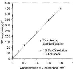
(7) List of figures. LIST OF FIGURES. Title. Figure 2.1. Page. Schematic representation of the tertiary structure of bovine 6. (3-lactoglobulin. 2.2. The effect of pH on the quaternary structure of (3-lactoglobulin. 7. 2.3. Modification of aroma compound retention according to structural modifications of (3-lactoglobulin with pH between 3 and 11.. 8. Hummel and Dreyer type chromatograms obtained for 40 and 80 ppm ethyl benzoate concentration in the eluent. 16. 2.5. Various components of the SPME device. 20. 2.6. Temperature dependence of the adsorption versus time profiles obtained for methamphetamine. 22. 2.7. Demonstration of myoglobin (M) and cytochrome (C) displacement by lysozyme (L) with time (A) and protein extraction using a polyacrylicacid-coated fibre (B).. 22. 2.8. Adsorption curve under different convection conditions. 23. 2.9. Boundary layer model. 24. 2.10. SPME configuration. 25. 3.1. Typical GC response (ethanol+ 2-heptanone). 32. 3.2. Typical GC response (ethanol+ 2-nonanone). 33. 4.1. SPME results for different sub-samples of 0.6 mM 2-heptanone standard solution. 37. Effect of extraction time at 25°C for 2-heptanone on the SPME results. 39. Effect of extraction time at 25°C for 2-nonanone on the SPME results. 39. 4.4. GC response curve of 2-heptanone standard solution. 40. 4.5. GC response curve of2-nonanone standard solution (7 µm PDMS coating fibre, extraction time 5 minutes). 41. 2.4. 4.2 4.3. Vll.

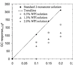
(8) List of figures. 4.6 4.7 5.1 5.2. GC response curve of2-nonanone standard solution (30 µm PDMS coating fibre; extraction time: 5 min). 42. GC response curve of 2-nonanone standard solution (30 µm PDMS coating fibre, extraction time: 30 seconds). 43. The effect of the addition of ethanol to 0.2 mM 2-nonanone standard solution on the GC response. 48. The effect of ethanol addition to a flavour-protein solution on the GC response. 49. The effect of ethanol addition to a flavour-protein solution on the GC response (0.2 mM 2-nonanone in 2% WPI solution; 30 µm PDMS fibre; extraction time: 5 min). 50. The interaction between WPI and 2-heptanone with time (0.4 mM 2-heptanone solution; 100 µm PDMS fibre; extraction time: 5 min). 52. The interaction between WPI and 2-heptanone with time (0.8 mM 2-heptanone solution; 100 µm PDMS fibre; extraction time: 5 min). 52. The interaction between WPI and 2-nonanone with time (0.2 mM 2-nonanone solution; 30µm PDMS fibre; extraction time: 5 min). 53. The interaction between WPI and 2-nonanone with time (0.2 mM 2-nonanone solution; 30µm PDMS fibre; extraction time: 30 seconds). 53. SPME results for the binding of2-heptanone to Na-CN (lOOµm PDMS fibre; extraction time: 5 min). 54. 5.9 5.10. Figure 5.9. SPME result for the binding of2-nonanone to Na-CN. 55. Klotz plot for 2-nonanone binding to Na-CN. 56. 5.11. SPME result of the binding of 2-heptanone to WPI (100 µm PDMS fibre; extraction time: 5 min). 57. SPME result of the binding of 2-nonanone to WPI (30 µm PDMS fibre; extraction time: 5 min). 57. SPME result of the binding of 2-nonanone to WPI (30 µm PDMS fibre; extraction time: 30 seconds). 58. Amount of bound 2-nonanone at different WPI concentrations. 58. Klotz plot for 2-heptanone binding to WPI. 60. Klotz plot for the binding of 2-nonanone to WPI at WPI concentrations ~ 0.5%. 61. 5.3 5.4 5.5 5.6 5.7 5.8. 5.12 5.13 5.14 5.15 5.16. Vlll.

(9) List of figures. 5.17. Klotz plot for the binding of 2-nonanone to WPI at WPI concentrations ;;:: 1 %. 5.18. Klotz plot for 2-nonanone binding to J3-lactoglobulin in WPI, assuming that all the binding occurred with J3-lactoglobulin alone at WPI concentrations ~ 0.5% Klotz plot for 2-nonanone binding to J3-lactoglobulin in WPI, assuming that all the binding occurred with J3-lactoglobulin alone at WPI concentrations ;;:: 1%.. 5.19. 62. 63 64. The proportion of monomer J3-lactoglobulin as a function of the protein concentration (simulated data using an association constant K = 4.88 x 104 M-1). 65. 6.1. The effect of pH on the binding of2-nonannone to WPI (1 %). 68. 6.2. Klotz plot for 2-nonanone and WPI binding at pH = 3. 69. 6.3. Klotz plot for 2-nonanone and WPI binding at pH= 4. 69. 6.4. Klotz plot for 2-nonanone and WPI binding at pH= 6. 70. 6.5. WPI-2-nonanone binding parameters at different pH values. 71. 6.6. Klotz plot for binding of 2-nonanone to J3-lactoglobulinbinding in WPI solution at pH = 4. 72. 6.7. Klotz plot for binding of 2-nonanone to J3-lactoglobulin in WPI solution at pH = 6. 73. 6.8. The effect of sodium palmitate on the binding of 2-nonanone to WPI. 76. 6.9. The effect of added sodium palmitate on J3-lactoglobulin2-nonanone binding. 78. 6.10. Comparison of the competition model and experimental results (0.5% WPI, 0.2 mM 2-nonanone). 81. 5.20. IX.

(10) LIST OF TABLES. Table. 2.1. Title. Page. Comparison of binding constants obtained with different methods. 12. 3.1. Temperature and conditioning recommendations for fibres. 30. 3.2. Retention times for the two components in standard solutions. 33. 3.3. Retention times of individual components. 34. 4.1. Container and liquid amount used for optimization of SPME conditions. 36. 4.2. The SPME-GC results obtained using different containers. 36. 4.3. The SPME results for 2-heptanone standard samples. 40. 4.4. The SPME results of 2-nonanone standard samples. 41. 6.1. WPI-2-nonanone binding parameters at different pH values. 70. 6.2. (3-Lactoglobulin-2-nonanone binding parameters at different pH. 72. values. 6.3. Bound amount of 2-nanonone in different sodium palmitate added. x. 80.

(11) Chapter One. futroduction. CHAPTER ONE INTRODUCTION. Flavour is an important quality factor of food products. Flavour binding to protein may change the flavour profile of food products, especially for new products. fu many new food products, additional proteins are often added to make the food more nutritious. However, sometimes the binding between flavour and protein can make the food lose its flavour balance and make the food lack flavour.. The interaction of flavour with protein has been the focus of research for a long time (Franzen and Kinsella, 1974). Much research has focused on. ~-lactoglobulin,. not only. because the binding can be easily detected but also because the well-studied structure of ~-lactoglobulin. makes it possible to investigate in detail the chemistry of flavour-protein. binding (Papiz et al., 1986).. Several techniques have been used to investigate the interaction between ~-lactoglobulin and flavours: these include equilibrium dialysis (O'Neill and Kinsella, 1987), static headspace (Charles et al., 1996), fluorimetry (Muresan and Leguijt, 1998), affinity chromatography. (Sostmann. and. Guichard,. 1998),. dynamic. coupled. liquid. chromatography (Jouenne and Crouzet, 1998) and exclusion chromatography (Pelletier et al., 1998). The results published for the same flavour compound interacting with. ~. lactoglobulin under certain experimental conditions were different, mostly because of the different techniques used (Guichard & Langourieux, 2000). Hence determing an efficient and reliable method of analysis is important.. Solid-phase microextraction (SPME) has been used in flavour analysis for more than 10 years (Arthur and Pawliszyn, 1990; Martos and Pawliszyn, 1997). It is a simple analytical tool and is relatively cheap. It is a solventless extraction method and increased sensitivity. 1.

(12) Chapter One. futroduction. and precision can be obtained with a suitable fibre and optimal experimental conditions (such as the temperature, the extraction time etc.). SPME is a convenient method for an experienced person. However, the experimental conditions must be optimized at the beginning of the analysis of a new system. The SPME process is very complex: adsorption, diffusion and desorption occur during SPME. As each process is important for the analysis, SPME is sometimes regarded as a technique that is not convenient for an inexperienced person.. Although there is much published work on the binding between. ~-lactoglobulin. and. flavours, in the food industry, commercial protein products are not pure products like. ~. lactoglobulin, and therefore establishing how protein products interact with flavour compounds is of real interest to the food industry. There is no published work on the use of SPME to investigate dairy protein-flavour binding.. This investigation on the interaction between flavour and dairy protein products (such as whey protein isolate and sodium caseinate) using SPME was a pilot study in the field and the results obtained will be useful to the food industry.. 2.

(13) Chapter Two. Literature Review. CHAPTER TWO. LITERATURE REVIEW 2.1 Flavour-matrix interactions Flavours are usually volatile chemical compounds that occur in very low concentrations (parts per million (ppm) or even parts perbillion (ppb )) in foods. These flavour compounds are not just mechanically trapped; they often interact with the matrix.. Lipids may be the most important factor affecting the flavour profile of a food product, because many of the naturally occurring flavour compounds are lipid soluble. However, as the development of new food products and ingredients has increasingly been aimed at enhanced nutrition, improved flavour and low fat, an understanding of the interactions between flavour and the food matrix will enable the manufacture of fat-reduced and fatfree products with satisfactory flavour profiles. It is also known that many non-volatile food ingredients, such as proteins and starch, influence the flavour of a food product (Wassef and Nawar, 1971; Franzen and Kinsella, 1974; Gremli, 1974). Early research focused on some proteins that bind flavour compounds in an easily detectable manner; soy protein and f3-lactoglobulin were the proteins of interest. Recently, ovalbumin and 11 S globulin have been studied (Adams et al., 2001; Semen ova et al., 2002). The quantitative binding parameters (the total number ofbinding sites in the protein molecule, the intrinsic binding constant and the Gibbs' free energy of binding) of some :flavours have been published (O'Neill and Kinsella, 1987).. 2.2 Interactions of volatile flavours in aqueous solution The concentration of flavour above the surface in aqueous solutions (headspace) can be easily theoretically predicted. From gas-liquid equilibrium (GLE) theory, the partition coefficient between the gaseous and liquid phases (Kgz} for a volatile compound (i), for. 3.

(14) Literature Review. Chapter Two. example, can be either measured directly in a system by determining the concentrations of (i) in the gaseous and liquid phases (equation 2-1) or calculated from :fundamental physicochemical parameters according to equation 2-2:. c~ I. 2-1. c'. I. 2-2. where P°i(T) is the vapour pressure (Pa) of pure (i) at temperature T, Pr, is the total pressure (Pa) in the gaseous phase and Vi and Vg are the molar volumes (m3 .mor1) of the liquid and the gaseous phase respectively. Normally, as the volatile compound is highly diluted in the liquid phase, the activity coefficient. ncan be assumed to be independent of. the concentration of the volatile compound in the liquid, and is equal to a constant. nro· Pi(T) is a constant (Henry's constant), so that the value ofK!gl depends only on the temperature. In all but the simplest systems, ndepends valuenro. In this case, the product. on the other components present in the aqueous phase and its value varies from the ideal value of 1. Although partition data can be calculated, experimental data are also required to check that the value chosen for. n is appropriate and to ensure that no other unknown. interactions are occurring.. The partition of volatile compounds is affected by soluble non-volatile flavour components such as sugars, acids, proteins and salts. There have been many papers on the subject since Buttery and his group (1971) reported changes in the headspace concentration of a flavour compound caused by its interactions with food components. In the dairy field, an understanding of the protein-flavour interaction in aqueous solution will be very useful for new product development because many products are water based.. 4.

(15) Literature Review. Chapter Two. It is worth pointing out that food systems are not usually equilibrium systems, because. not enough time is available for the equilibrium to be reached in the mouth while the food is consumed. This particular case comes within another area of flavour research (flavour release) and is not discussed in this work.. 2.3 Mechanism of binding of ligands to. ~-lactoglobulin. B-Lactoglobulin is the most used dairy protein in flavour binding research. Flavour-protein binding is actually related to the chemical properties and the structures ofboth the flavour compounds and the proteins. For example, it has been pointed out that B-lactoglobulin binds some hydrophobic ligands (Cho et al., 1994) in its hydrophobic pocket. Therefore, an understanding of the structure of the molecule is vital for understanding of the binding mechanism.. 2.3.1 The structure of ~-lactoglobulin and the binding sites B-Lactoglobulin is one of the major proteins in bovine milk, accounting for more than 50% of the total whey proteins and 10% of the total proteins of milk (Rambling et al., 1992). The amino acid sequence (Swaisgood, 1982) ofbovine B-lactoglobulin consists of 162 residues per monomer. The isoionic point of bovine B-lactoglobulin is pH 5.2 (Cannan et al., 1942). It is a typical globular protein and its structure has been extensively studied (Papiz et al., 1986). B-Lactoglobulin is a highly structured protein: optical rotary dispersion and circular dichroism measurements show that, at pH in the range 2-6,. B-. lactoglobulin consists of 10-15% a-helix (Frushour and Koenig, 197 5), 43 % B-sheet and 47% unordered structure (Townend et al., 1967), including B-turns. The tertiary structure of B-lactoglobulin is a very compact structure in which the B-sheets occur in a B-barreltype or calyx (Figure 2.1 ). Each monomer exists almost as a sphere with a diameter of about 3 .6 nm. There is a hydrophobic pocket in the tertiary structure of B-lactoglobulin (Papiz et al., 1986). Many hydrophobic molecules including retinol (vitamin A) and free fatty acids have been shown to bind inside this pocket (Fugate and Song, 1980; Puyol et. al., 1991 ). Similarly, some hydrophobic flavours have been found to bind to. 5. B-.

(16) Literature Review. Chapter Two. lactoglobulin (Futterman and Heller, 1972); however, unlike retinol and free fatty acids the binding positions for these flavours have not been reported.. B. molecule. Figure 2.1. Schematic representation of the tertiary structure of bovine f3-lactoglobulin, showing the binding of retinol; the arrows indicate antiparallel f3-sheet structures (from Papiz et al, 1986).. It can be assumed that the flavour should bind within the hydrophobic pocket; however, binding of the flavour could take place not only inside the pocket but also at some other sites on the surface of the molecule. Narayan and Berliner (1997) found at least two different types of simultaneous hydrophobic ligand binding sites and pointed out that there are also several weaker sites for 5-doxylstearic acid. Sawyer and coworkers (1998) identified three distinct sites with the two main sites being the retinol site (in the centre of the f3-barrel) and another site on the outer surface close to the helix. They described the 6.

(17) Chapter Two. Literature Review. three kinds of binding sites as the retinol binding site, the fatty acid binding site and the polar aromatic binding site. However, it is still unclear where the binding sites for flavour compounds are on 13-lactoglobulin.. 2.3.2 Effect of pH on ligand binding pH is an important factor in the binding of ligands to 13-lactoglobulin (Sostmann and Guichard, 1998). It has been found that the quaternary structure of 13-lactoglobulin changes with changes in pH.. 8. Dimer (pl f 5.5-7.5). Octa mer {pI I 3.5-5.5). 1. J. 0. 0. Monomer (pH<3.5). Monomer (pl!> 75). Figure 2.2. The effect of pH on the quaternary structure of f3-lactoglobulin (Fox and Mcsweeney, 1998). 13-Lactoglobulin is a dimer at physiological pH (Fox and Mcsweeney, 1998). Below pH 3.5, 13-lactoglobulin dissociates to monomers with a molecular mass of18 kDa. Between pH 3.5 and pH 5.2, 13-lactoglobulin occurs as octamers of molecular mass 144 kDa. Between pH 5.5 and pH 7.5, 13-lactoglobulin forms dimers of molecular mass 36kDa.. 7.

(18) Chapter Two Above pH 7.5,. Literature Review ~-lactoglobulin. dissociates to monomers. The association of. ~. lactoglobulin as a function of pH is summarized in Figure 2.2.. It is likely that the binding ligands will be affected by the changing structure of. ~. lactoglobulin as the pH changes. Jouenne and Crouzet (2000) proposed the relationship between structure and binding shown in Figure 2.3. Retention%. Primary site Junction area Band I. 7,5. 3. Tanford Transition. 6. ~ Compact and rigid tertiary structure. @. @ Flexible tertiary structure, exposition. @. of hidden residues, ionization. · ··. .. Alkaline denaturation ~. pH 11. Partial unfolding, ionization. Total unfolding of 13-sheet, modification of the hydrophobic cavity structure. Figure 2.3. Modification of aroma compound retention according to structural modifications of. ~-lactoglobulin. with pH between 3 and 11. Site accessibility: (+). medium; (++) high; (+++) very high; (±) more or less important (Jouenne and Crouzet, 2000).. Around pH 3, the tertiary structure of. ~-lactoglobulin. is compact and rigid. The. accessibility of the binding sites is medium for the first binding site and high for the second binding site. Around pH 6, the tertiary structure of~-lactoglobulin is flexible, the hidden residues are exposed and the molecules are partly ionized. The accessibilities of the binding sites are high for both the first and second binding sites. Around pH 9, the. 8.

(19) Literature Review. Chapter Two. tertiary structure of 13-lactoglobulin is partially unfolded and the molecules are ionized; the accessibility of the first binding site is very high and the second binding site is damaged. Above pH 11, the tertiary structure of 13-lactoglobulin is totally unfolded 13sheet and the hydrophobic cavity structure is modified. The accessibility of the first binding site is more or less important.. 2.4 Equilibrium binding phenomena The most commonly used method for interpreting binding data makes use of the Scatchard (1949) equation. This model is based on two assumptions: that each of the protein molecules has n indistinguishable and independent binding sites; that the binding is an equilibrium (reversible) binding. For a system consisting of protein and flavour, when equilibrium is reached, the concentrations of protein and flavour are P and L respectively, and the equilibrium for one binding site can be expressed as. P+L. ~PL. According to equilibrium theory,. K = [PL] [PJL]. 2-3. where K is the equilibrium constant. Therefore. [PL]=K[P]·[L]. 2-4. [PL]= K[L]. [~oral - PL]. 2-5. As P1ora1=P+PL,. 9.

(20) Chapter Two. Literature Review. or. [PL]. [~otal]. K[L] = I+K[L]. 2-6. Now,. [PL] --=v. 2-7. [~otal]. where vis the number of moles ofligand bound per mole of total protein. Thus:. K[L] - I+K[L]. 2-8. v--~~. If there are n independent binding sites, the equation of the extent ofbinding is simply n. times that for a single site with the same intrinsic binding constant, K. Hence:. nK[L] I+K[L]. 2-9. v=-~~. or. v/L=Kn-Kv. 2-10. A plot of v/L against v gives the Scatchard plot. The equation may be rearranged to give:. 1 1 1 = +v nK[L] n. 2-11. A plot of 1/v againt I IL gives rise to the Klotz, or double reciprocal plot, in which the slope of the line is llnK and the intercept is lln (Klotz, 1946).. 10.

(21) Literature Review. Chapter Two. However, sometimes the plot will not be a straight line, because the different binding sites are not independent. In these circumstances, the Hill equation is applied (Hill, 1910):. n. 2-12. v=----. 1 +1 (K[L]t. 1. v. 1. 1. n(K[L]t. n. ---+-. 2-13. where h is the Hill coefficient reflecting the co-operation between the sites. The other parameters have the same meaning as in the Klotz plot.. 2.5 Published results on flavour-protein binding f3-Lactoglobulin has been well studied in flavour binding as a pure protein. However, as well as pure f3-lactoglobulin, other daicy products such as whey proteins and casein are of great interest.. Several methods have been used to analyse the interaction between f3-lactoglobulin and flavours. Up to now, the results reported have been more or less different because different methods have been used, which is an indication that not all the methods available are reliable. Some of the published results selected from the literature can be found in Table 2.1 and illustrate how much work still needs to be done with respect to technique development in spite of the many papers published in this field. Binding parameters detected under different conditions (such as equilibrium temperature, pH), using different methods, will have different meaning. It is vecy difficult to determine out which method is the most reliable and appropriate to use.. 11.

(22) Literature Review. Chapter Two. Table 2.1. Comearison of binding constants obtained with different methods. Flavours. Method. Conditions. pH= 3 at room temperature. n.d.. 341*. Exclusion chromatography (Pelletier et al., 1998). pH= 3 at room temperature. 0.3. 1800 M-1. Static headspace (Charles et al., 1996). pH=3 at 30°C. 0.57. 533 M- 1. Fluorescence (Muresan and Leguijit, 1998). Not mentioned. 0.8. 2.5x10 6 M-1. pH=6.7 at 25°C. 1. 150 M- 1. pH=3 at room temperature. n.d.. pH=6.7 at 25°C. 1. pH= 3 at room temperature. n.d.. 1287 M- 1. pH=6.7 at 25°C. 1. 2440 M- 1. Benzaldehyde Affinity -chromatography (Sostmann and Guichard, 1998). 2-Heptanone. Equilibrium dialysis (O'Neill and Kinsella, 1987) Affinity -chromatography (Sostmann and Guichard, 1998). 2-0ctanone. Equilibrium dialysis (O'Neill and Kinsella, 1987) Affinity -chromatography (Sostmann and Guichard, 1998). 2-Nonanone. Binding Binding sites constants n Kb. Equilibrium dialysis (O'Neil and Kinsella, 1987). 465 * 480 M- 1. Affinity-chromatography pH=3 at room (Sostmann & Guichard, 1998) temperature. n.d.. 3629 *. Equilibrium dialysis (Muresan et al., 1999). pH=3 at room temperature. 0.5. 1756 M- 1. pH=3 at 30°C. 0.5. 1667 M- 1. n.d.. 4433*. Static headspace (Charles et al., 1996) 2-Nonenal. Affinity -chromatography (Sostmann and Guichard, 1998). pH= 3 at room temperature. a-Ionone. Fluorescence (Dufour and Haertle, 1990). Not mentioned. Affinity-chromatography (Sostmann and Guichard, 1998). 12. pH=3 at room temperature. 0. n.d.. 13456 *.

(23) Literature Review. Chapter Two. Table 2.1 (continued) f3-Ionone. Fluorescence (Dufour and Haertle, 1990). Not mentioned. 1.08. 1670000. Fluorescence (Muresan and Leguijit, 1998). Not mentioned. Affinity -chromatography (Sostmann and Guichard, 1998). pH= 3 at room temperature. n.d.. 19143*. Equilibrium dialysis (Muresan et al., 1999). pH= 3 at room temperature. 0.9. 11700 M- 1. M-1. 0.8. 1.9x106 M-1. * The binding constant obtained using affinity chromatography is presented as the product nKb. n.d. = not determined.. Milk protein products, such as sodium caseinate (Na-CN) and whey protein concentrate (WPC) have also been investigated for their interaction with flavour using different methods. In contrast to the methods mentioned above, sensory panels have been used. Hansen and Heinis (1991) used sensory evaluation to investigate the interactions ofNaCN and WPC with vanillin. The vanillin-Na-CN and vanillin-WPC solutions contained 78.5 ppm vanillin, 2.5% sucrose, and 0.125, 0.25 or 0.5% Na-CN or WPC. A 12-member trained panel evaluated the samples at room temperature and found that the vanillin flavour intensity was moderately less than the vanillin reference for all Na-CN levels. As the WPC concentration increased from 0.125 to 0.5%, the vanillin flavour intensity decreased from moderately less than the vanillin reference to much less than vanillin reference.. Fares et al. (1998) studied the physico-chemical interactions between aroma compounds and Na-CN by complementary techniques involving the protein in aqueous solution at 25 or 75 g/L (exponential dilution and equilibrium dialysis) or in a solid state (sorption and infrared spectroscopy). Diacetyl and benzaldehyde were found to interact with Na-CN through strong and weak bonds in aqueous solution. Although no retention ofacetone and. 13.

(24) Literature Review. Chapter Two. ethyl acetate was found in aqueous solution, the compounds that sorbed best to Na-CN in the solid state were acetone and ethyl acetate.. 2.6 Analysis methods As mentioned previously, several instrumental methods for detecting flavour-protein. binding have been reported. Each method has its benefits and shortfalls. The basic principles of these methods are discussed below.. 2.6.1 Fluorescence Fluorescence can be used to detect the concentration of protein in solution. However, when some flavour compounds bind to protein, the fluorescence intensity changes at a fixed wavelength. For example difference in fluorescence intensity at 332 nm between complexed and free f3-lactoglobulin has been monitored to determine apparent dissociation constants of various ligands complexed by the protein (Fugate and Song, 1980; Dufour and Haertle, 1990). It was assumed that the change in fluorescence depended on the amount of protein-ligand complex, and the apparent dissociation constants were obtained according to the method of Cogan et al. (1976):. K/ = (a/1-a)[B-nPa(l-a)}. 2-14. which can be rearranged to. Paa. lln[B(a/1-a}]-(K/!n). 2-15. where K/ is the apparent dissociation constant, n is the number ofindependent binding sites and Pa is the total protein concentration. a is defined as the fraction of free binding sites in total binding sites on the protein molecules. The value of a was calculated for every desired point on the titration curve of fluorescence intensity versus total ligand concentration using the relation:. 14.

(25) Literature Review. Chapter Two. 2-16. where F represents the fluorescence intensity at the certain total ligand concentration B,. F0 is the fluorescence of the free protein and Fmin represents the fluorescence intensity upon saturation of all the protein molecules. A plot of P0 a against B(a/1-a) yields a straight line with an intercept of K/!n and a slope of 1In.. Dufour and Haertle (1990) studied interactions of P-ionone and related flavour compounds with P-lactoglobulin. In their work, the independent binding sites and dissociation constants were calculated (see Table 2.1 ). Muresan and coworkers (1999) published their binding constants and binding sites. It can be seen in Table 2.1 that the binding constants obtained from fluorescence measurements are much higher than those obtained using other techniques.. 2.6.2 Affinity chromatography Affinity chromatography is a well-known method that immobilizes the protein in the column. Sostmann and Guichard (1998) first used this technique to investigate flavour-protein binding. The most important step in the experimental process is immobilization of the protein in the column. After the immobilization is achieved, the determination is fast and convenient.. Calculation of the binding constants (Kb), given by Nilsson and Larson (1983), is as follows:. 2-17 where Cp is the concentration of protein, t 0 is the void time and fR represents the retention time of the compound. The void time can be determined by injection of water on to the column and can be used for calculation of the column void volume. 15.

(26) Chapter Two. Literature Review. Retention times can be determined by two methods because the support material (normally silica-diol or silica gel) is not inert to all flavour compounds, which causes some compounds to be retained by the column: (i) experimentally, by applying a chromatographic material treated using the same conditions as for immobilization of the protein, but without protein in the treatment solution; (ii) by determining the linear relationship between protein content and retention time for each compound at more than five different protein concentrations and calculating the retention time for zero protein concentration. The two methods should give results that are in good agreement.. Ethyl benzoate. Ethyl benzoate 40ppm. 80ppm. a Without. P-lactoglobulin I.' 'I·. j. m.. I. I. J ' ~. I. I. 1 1 1'1'.:'1·;. I Ii H. I. I I. I. l. ••£~••••I~. • • 0 CJM. .. d. b. With. P-lactoglobulin ( l % ). [. ( I 'I. i. •. 8. i'l·t t a •. D M. 'I. I. l'l'1. U. •. •. •. I. \ J-~. 11 11. 1·1·1 1 1. c •. • •. •. i'l. •. •. •. •. I. •. I. •. Figure 2.4. Hummel and Dreyer type chromatograms obtained for 40 and 80 ppm ethyl benzoate concentration in the eluent: injection of ethyl benzoate 40 ppm without ~-lactoglobulin (a) or With ~-lactoglobulin (b); injection of ethyl benzoate 80 ppm without ~-lactoglobulin (c) or with ~-lactoglobulin (d). 16.

(27) Literature Review. Chapter Two. One shortfall of this method is that no information about binding sites can be obtained. To overcome that limitation, Pelletier et al. (1998) used the Hummel and Dreyer method (1962) to calculate the number of binding sites. In their study, injection of. ~. lactoglobulin with the esters led to the observation of a negative peak (Figure 2.4) corresponding to the bound ester. The amount of bound ester was determined by internal calibration. Different concentrations of ester in the eluent (free ester) were used to develop a Klotz plot.. Affinity chromatography is a rapid method for detecting flavour-protein binding. The data obtained are reproducible. The number ofbinding sites and the affinity constants can be calculated using the Hummel and Dreyer method, when possible.. 2.6.3 Headspace techniques The static headspace technique is based on gas-liquid equilibrium (GLE) theory. When the headspace of the sample is in equilibrium with the sample solution, the concentration of the flavour in the headspace corresponds to the concentration of the free flavour in the sample solution. For detection of the binding, a standard curve is drawn. The response of the standard minus that of the corresponding sample is regarded as the binding response. The concentration of free flavour is calculated using the following equation (O'Keefe et al., 1991):. 2-18. L = (RIT)I. where R (mol.r 1) is the measured concentration of :flavour in the headspace of the protein solution, T (mol.r 1) is the measured concentration of :flavour in the headspace of the solution without protein (standard solution) and I (mol.r 1) is the initial concentration of flavour in the solution (concentration of the standard solution).. 2.6.4 Equilibrium dialysis 17.

(28) Chapter Two. Literature Review. Equilibrium dialysis (O'Neill and Kinsella, 1987) has been used to determe the binding constants and binding sites of J3-lactoglobulin for different flavour compounds. Usually, acrylic cells of equal volume, separated by a membrane and belted together, are put into a waterbath. A defined volume of solution (1 ml for example) containing the flavour compound only is put into one side of the membrane, and the same amount of solution containing protein only is placed into the other side of the membrane. The cells are then shaken for 20-40 h at the required temperature (25°C for example) to attain equilibrium between the flavour and the protein. Aliquots are then removed from each compartment, placed in vials and extracted using an extractant (e.g. isooctane). Gas chromatography is used for quantitative determination of the amount of flavour in each compartment. The difference in the concentrations of the flavour compound in the respective compartments relates to the amount of flavour compound bound by the protein.. Headspace analysis has played a key role in flavour-protein binding research. However, there are still several major experimental limitations (O'Neill, 1994). Generally, because the concentration of flavour compounds in the sample is quite low, a large sample volume is needed for adequate detection, which can affect the chromatographic analysis. To overcome this shortfall, a better analysis technique is needed.. 2. 7 Solid-phase microextraction technique Solid-phase microextraction (SPME) is a solventless extraction method (Arthur and Pawliszyn, 1990; Arthur et al., 1992). It is inexpensive and rapid. It can be used both for the headspace of the sample, as the HS-SPME method, and for a liquid sample directly (Yang and Peppard, 1994; Steffen and Pawliszyn, 1996). Because the components in the solution can sometimes affect the analysis results (for example, in a protein solution, protein may be adsorbed to the fibre and make the analysis incorrect), SPME is mostly used with the headspace option.. 18.

(29) Chapter Two. Literature Review. The principle of the technique is based on adsorption theory. A fibre coated with a defined volume of adsorbent is put into the headspace of the sample for extraction. The extraction needs to be carried out under defined conditions (temperature, sample volume, container shape and volume, time of extraction) to make the analysis reproducible. After extraction, the fibre is transferred into a gas chromatograph for analysis. It is not like a traditional solvent extraction where the sample must be extracted completely to maintain the accuracy of the determination. SPME is a partial extraction method. The amount of analyte remaining after SPME does not affect the result of the SPME determination under defined conditions.. 2. 7.1 Equilibrium sampling Figure 2.5 shows the various components of the SPME device. A fibre coated with adsorbent is attached to the plunger of a modified syringe. The fibre is sheathed in a stainless steel septum-piercing needle. When sampling, the septum of the sample is pierced by the needle and the fibre is then pushed out of the sheath. Several different kinds of fibres coated with different materials are now available commercially.. In a closed system consisting of only the sample and the SPME fibre, the following. relationship exists if the sampling time is sufficiently long to allow equilibrium to be established between the sample and the fibre:. (K JsV1 VsC0. n = (KfsV! +. ). 2-19. vJ. where n is the mass of flavour compound extracted by the fibre coating,. Krs. is the. partition coefficient of the flavour compound between the fibre and the sample (distribution constant), 1j and Vs are the volumes of the fibre coating and the sample respectively and Ca is the initial concentration of the flavour compound in the sample.. 19.

(30) Chapter Two. Literature Review. plunger. syringe barrel. stainless steel needle/ wire attached to fibre /. __.. fibre and coating /. Figure 2.5: Various components of the SPME device. In practice, two different situations can occur. When Vs is much greater than K1s· Vj,. equation 2-19 can be simplified to:. 2-20. In this case, the results are not affected by the volume of the samples.. If Vs is not very large, the concentration of the samples will change when the samples are. extracted by the SPME fibre. In this case, the results will change with the volume of the samples. The same amount ofliquid sample and the same size and shape of the container should be used to obtain reproducible results. 20.

(31) Literature Review. Chapter Two. For. 2-21. ifthe volume of the sample (Vs) is maintained the same during the determination, then k will be a constant. Equation 2-19 can be simplified as:. 2-22. The principle of SPME is similar to those of traditional extraction techniques and it is a successful method. Unlike the traditional extraction method, SPME can also be used as dynamic system (rapid sampling).. 2. 7 .2 Dynamic sampling (rapid sampling) It may take a long time before equilibrium is reached in a system. Figure 2.6 illustrates equilibrium time profiles obtained for the extraction of methamphetamine at various temperatures. Generally, the higher the temperature, the shorter is the equilibrium time (Pawliszyn, 2000).. From Figure 2.6, we can see that, even in the fastest case, at a temperature of 73 °C, the equilibrium time for extraction can be less than 20 min; it is not the exact thermodynamic equilibrium time, but it works well for analysis. In the low temperature case, for example at 22 °C, the equilibrium time is more than 90 min, which is too long. In this situation, the rapid sampling (dynamic sampling) method should be applied.. 21.

(32) Literature Review. Chapter Two. --. ~ 450. 1l. -.. c. e. >< ~. 40Q ~50. •. 300. !II. c. em 250. Qi. 200. ,t;:; Q.. E 150. l'!!. .c O>. :::. 100 50. 0. 0. 20. 40. 60. 100. 80. Time (min). Figure 2.6. Temperature dependence of the adsorption versus time profiles obtained for methamphetamine (Pawliszyn, 2000). Temperature: • 22°C •40°C 111160°C • 73°C. A. B. c. L L. l. M. L __.....__..__-41..,.. min 0. 5. t.i;;;: 240 s. 10. Figure 2. 7. Demonstration of myoglobin (M) and cytochrome (C) displacement by Iysozyme (L) with 1ime (A) and protein extraction using a polyacrylicacid-coated fibre (B) (Pawliszyn, 2000).. 22.

(33) Chapter Two. Literature Review. The other reason for using a short extraction time is for the analysis of a multi-component system. In the case of more than one component in the system, the competition among these components is quite important. If SPME is to be used to extract a mixture that contains, for example, the three compounds myoglobin, cytochrome and lysozyme, only the compound with the weakest affinity will be observed at short extraction times (illustrated in Figure 2.7). When the extraction time is longer, the analytes that have lower affinities will be displaced by the analyte that has higher affinity for the polyacrylic-acid-coated fibre. In this case, lysozyme (having the strongest affinity) will replace the other two compounds during the extraction. This occurs because, at the beginning of the extraction, all the surface of the fibre is free, and all the analytes can be adsorbed by the fibre; when the whole surface of the fibre is occupied by the analytes, the analyte with strong affinity for the fibre will displace the analytes with weaker affinity for the fibre. Therefore, the equilibrium amount extracted may vary with the concentration of both the target and other analytes (Liao et al., 1996; Gorecki et al., 1999).. Good convection ~condition. Extraction time Figure 2.8. Adsorption curve under different convection conditions (imaging). • Transit time; a Typical extraction time for equilibrium sampling; o Typical extraction time for dynamic sampling.. 23.

(34) Chapter Two. Literature Review. The short-time-exposure HS-SPME measurement (dynamic sampling) 1s used to overcome the shortfall mentioned above. The short time extraction avoids the replacement by the stronger analytes (Figure 2. 7). When performing such an analysis it is critical not only to precisely control the extraction times, but also to monitor the convection conditions to ensure that they are constant. Figure 2.8 illustrates the difference between equilibrium sampling and dynamic sampling. fu the equilibrium system, the extraction time must be longer than the transit time. Although equilibrium has not been reached after the transit time, it is precise enough for the determination because the amount of analyte adsorbed changes very slowly with the extraction time after the transit time.. fu the dynamic system, the extraction time is very important for the analysis. It can be. seen in Figure 2.8 that the slope of the adsorption curve is quite steep in dynamic sampling. A small difference in the extraction time may cause a big difference in the amount adsorbed. The convection condition is also an important factor that must be taken into account. fu Figure 2.8, the same extraction time, but under different convection conditions, would result in totally different results. fu dynamic sampling, the whole adsorption process can be simplified as in Figure 2.9 (Pawliszyn, 2000).. Fibre core /iFibre coating. Boundary layer. Sample. Distance Figure 2.9. Boundary layer model (Pawliszyn, 2000).. 24.

(35) Literature Review. Chapter Two. The mass of extracted analyte can be estimated from the following equation:. n(t). =. {21CD/.Jln[(b+5)/b]} ·Cgt. 2-23. In this situation, agitation affects the boundary thickness ( b), which is the important. factor in equation 2-23. A diffilsion coefficient is used in equation 2-23, rather than distribution coefficients.. If the amount adsorbed in sampling is large enough to have changed the concentration of. the headspace, the equilibrium between the liquid and the headspace will also affect the analysis result, because there are two different kinds of equilibrium, as shown in Figure 2-10, while HS-SPME is being conducted: vapour-solid-equilibrium (V-S-E) as mentioned above; liquid-vapour-equilibrium (L-V-E) between the liquid sample and its headspace. The latter equilibrium is usually reached before HS-SPME is applied.. V-S-E. L-V-E. Figure 2-10. SPME configuration. If the amount of analyte adsorbed is quite small, then the L-V-E is not affected and the. sampling process does not affect the L-V-E; a more complex case occurs when the amount ofanalyte adsorbed is not small enough, in which case L-V-E will be affected. In. 25.

(36) Literature Review. Chapter Two. this case, the analyte will escape from the water phase to the headspace to satisfy the LV-E while HS-SPME is being performed. The whole extraction process is too complex to describe using theory. In practice, it is hard to distinguish the two different kinds of sampling.. In summary, it is important when using HS-SPME to maintain all the conditions as. constant as possible, because it is difficult to establish whether or not the sampling process is carried out under equilibrium conditions. Even under the equilibrium conditions, L-V-E may be affected. Conditions to be kept constant include the amount of liquid used for one sample, the size and shape of the containers, the speed of the agitator for both liquid and vapour, the temperature of the extraction process and the time taken to prepare a sample ... 2.8 Conclusions In conclusion, it is apparent that HS-SPME in conjunction with gas chromatography. would be an appropriate method to use in flavour-protein binding research. There is only one reported study on flavour-protein (ovalbumin) binding using HS-SPME (Adams et al., 2001 ). The technique has the potential to be applied to dairy protein-flavour binding research.. Another potential application for the HS-SPME technique is in the area of quality control, where the method would be used to assess dairy products, especially new products based on the flavour analytes, and to determine whether the products would be acceptable to the consumer. The advantage of such a technique would be that the HS-SPME method would replace time-consuming and expensive to run sensory analysis. However, in order to use such an objective analytical tool to assess the flavour profile of dairy products, there are many steps that need to be taken to ensure that the analytical method is measuring exactly what the consumer perceives. Hence, it is important that the analytical and sensory responses are correlated before the analytical tool is used alone.. 26.

(37) Chapter Two. Literature Review. 2.9 Objectives The present study was divided into four sections, with four main objectives.. •. Development of a sampling methodology for HS-SPME. •. Investigation of whey protein isolate-flavour binding. •. Investigation of sodium caseinate-flavour binding. •. Mechanism of 13-lactoglobulin-flavour interaction. 27.

(38) Chapter Three. Materials and Methods. CHAPTER THREE. MATERIALS AND METHODS 3.1 General materials and equipment •. Whey protein isolate (WPI) and sodium caseinate(Na-CN) powders were obtained from Fonterra (New Zealand).. •. 4 ml glass vials with open-hole screw top lids were obtained from Alltech, and butyl rubber resealable septa were purchased from Chromspec Distributors (NZ) Ltd.. •. Distilled, deionized water (DDI) was obtained from a MilliQ filter system in the laboratory. Henceforth, the term "water" refers to DDI.. •. AnalaR grade ethanol was obtained from Sigma-Aldrich Fine Chemicals (St. Louis, Missouri, USA).. •. 2-Nonanone and 2-heptanone were food grade and were supplied by Sigma-Aldrich Fine Chemicals (St. Louis, Missouri, USA).. •. A Supelco (Bellefonte, Pennsylvania, USA) NukoI™ capillary column (15 m x 0.53 mm x 0.53 µm) was used throughout the experimental work.. •. The. manual. SPME. syringe. and. coated. fibres,. 100,. 75,. and. 30. µm. polydimethylsiloxane (PDMS) fibres, were purchased from Chromspec Distributors (NZ) Ltd.. 28.

(39) Materials and Methods. Chapter Three •. Nitrogen (oxygen-free, OFN) and hydrogen gas cylinders, hooked up to the gas chromatograph (GC), were supplied by BOC Gases (Palmerston North) Ltd.. •. A Heidolph waterbath ± 0.1°C was supplied by Watson Victor Ltd. New Zealand.. 3.2 Gas chromatography A Supelco Nukol™ capillary column (15 m x 0.53 mm x 0.5 µm) was used in the present study. The carrier gas used was OFN and while hydrogen and dry air were mixed in optimum proportions for use in the flame ionization detector (FID40). The flow rates of the carrier and fuel gases and the temperature were as follows: •. Nitrogen (carrier gas). 20 ml/min. •. Hydrogen (fuel). 50 ml/min. o. Make up. 35 ml/min. o. Dry air. 100 ml/min. •. Injector port temperature. 250°C. •. Detector temperature. 250°C. o. Maximum column temperature. 200°c. •. Oven temperature. 100°c. The splitless model was used, as the concentrations of the volatiles being analysed were very low (0-1 OOppm). This model allows the maximum volume of analyte to reach the detector from the injector port via the column. The column was conditioned overnight before commencing a batch of GC experiments. This was done by heating the column slowly (5°C/min ramp) to 195°C, holding it for lh and then cooling the column back down to 40°C. This cycle was carried out repeatedly throughout the night before the day of use, particularly if the GC had not been used for more than 2 weeks.. 3.3 Headspace solid phase microextraction. 29.

(40) Chapter Three. Materials and Methods. All the new fibres were conditioned before use to prolong their extraction abilities. Up to 50 or more injections were possible with each fibre after the conditioning treatment had been applied. The details of conditioning are shown in Table 3 .1.. Table 3.1. Temperature and conditioning recommendations for fibres Stationary phase. Film. Maximum Recommended Conditioning. Time. thickness. temperature. temperature. temperature. (h). 100 µm. 2so 0 c. 200-270°C. 250°C. 1. 30µm. 2so 0 c. 200-270°C. 250°C. 1. 7µm. 340°C. 220-320°C. 320°C. 2-4. PDMS/DVB. 65 µm. 210°c. 200-270°C. 260°C. 0.5. Polyacrylate. 85 µm. 320°C. 220-310°C. 300°C. 2. CAR/PDMS. 75 µm. 320°C. 240-300°C. 2so 0 c. 0.5. CW/DVB. 65 µm. 265°C. 200-260°C. 250°C. 0.5. 50130 µm. 270°C. 230-270°C. 270°C. 4. PDMS. DVB/CAR/PDMS. The analysis process consists of several steps, as follows.. 1.. SPME extraction The SPME fibre is put into the headspace of the sample at a constant temperature for a definite time. In this stage, the important factors are maintaining a constant extraction time for each sample, maintaining the same depth of fibre into the vials for each sample and not damaging the fibre while piercing and withdrawing the fibre through the septa of the vials.. 2. GC analysis The fibre is transferred into the injector port of the GC as soon as possible after the extraction is completed.. 30.

(41) Chapter Three. Materials and Methods. 3. Fibre purge and reuse The fibre is left in the port at 250°C for 5 min, and then withdrawn from the port. The fibre is kept on the bench for 15 min to cool to the room temperature before analysing the next sample.. 3.4 Standard solutions 3.4.1 Flavour compounds stock solution 0.01 M flavour compounds stock solutions were made by weighing 0.057 g 2-heptanone and 0.071 g 2-nonanone respectively into a 50 ml volumetric flask using the capillary technique (Bassette, 1984) and making up to the required volume with 30% and 50% ethanol solution respectively. The stock solution was stored at 5°C and was used as required. The solution was stable for up to 2 months at this temperature according to Ulberth (1991).. 3.4.2 External standard method The dynamic and equilibrium sampling SPME technique was used in this study. Calibration was performed for the GC and the SPME fibres. For every fibre, a calibration curve was prepared before analysis of the samples. 0.01 M stock solutions of the two flavour compounds were diluted with water to give 0.1, 0.2, 0.4, 0.6 and 0.8 mM standard solutions.. 0.4 ml of a standard solution was pipetted into a 4 ml glass vial and the vial was covered with a screw cap immediately. Different fibres were calibrated independently. Four subsamples were prepared for each solution.. 3.4.3 Protein solutions WPI and Na-CN solutions at 0.5,1,1.5 and 2% were prepared by weighing 2.5, 5, 7.5 and. 10 g powder into a beaker and adding 200 ml water. The solution was stirred for 1 h and then transfered to a 500 ml volumetric flask. The beakers were washed with water and the. 31.

(42) Materials and Methods. Chapter Three. wash water was transferred into the volumetric flask. The solutions were stored at 5°C for 6 h before using them to prepare the flavour-protein mixture solutions.. 3.4.4 Flavour-protein mixed solutions Flavour-protein binding was detected by comparing the SPME analysis of the standard flavour solution with that of a flavour-protein solution at the same flavour concentration at a given protein concentration. The flavour-protein solutions were made in the same way as the standard flavour solutions. For example, 0.1, 0.2 and 0.4 mM flavour in 1% WPI solutions were prepared by pipetting 1 ml stock solution into 100, 50 and 25 ml volumetric flasks and making up to the final volume with 1% WPI solution. The concentration of protein in the mixture solutions changed after mixing with 1 ml of stock flavour solution. The concentration ofWPI solution was calculated from the volume of each flask used. The samples were stored at 5°C for> 40 h.. 3.5 Determination of analyte retention times The retention time for a given analyte will be different under different GC conditions. The GC conditions used were as mentioned earlier, the samples were analysed at 25°C and were extracted for 5 min. Typical GC graphs are shown in Figures 3.1 and 3.2.. TOP Figure 3.1. Typical GC response (ethanol+ 2-heptanone).. 32.

(43) START. G.845. ..;TOP. Figure 3.2. Typical GC response (ethanol + 2-nonanone).. There were at least two components in each of the standard flavour solutions (i.e. the flavour compound and ethanol). Which peaks represented the target flavour compound, ethanol and other impurity components had to be identified. The obvious way would be to use GC-MS to identify the flavours. However, because there were only two major components in the solution, it was possible to use just the GC to identify the peaks. The components in the two standard flavour solutions and their retention times were as shown in Table 3.2.:. Table 3.2. Retention times for the two components in standard solutions Standard solutions. Retention times Peak 1. Peak2. 1. Ethanol+ 2-heptanone. 0.842 min. 1.35 min. 2. Ethanol+ 2-nonanone. 0.845 min. 2.72 min. Although the retention times of peak 1 were slightly different, it was still quite clear that this was the retention time of ethanol. In fact, the retention times of all analytes will differ slightly in different analyses. The retention times of the analytes are listed in Table 3.3.. 33.

(44) Chapter Three. Materials and Methods. Table 33. Retention times ofindividual components Analyte. Retention time (Rn. Ethanol. ~0.84min. 2-Heptanone. ~1.35. min. 2-Nonanone. ~2.72. min. 34.

(45) Chapter Four. Optimization ofSPME Conditions for Flavour Binding Analysis. CHAPTER FOUR OPTIMIZATION OF SOLID PHASE MICROEXTRACTION CONDITIONS FOR FLAVOUR BINDING ANALYSIS 4.1 Introduction Suitable conditions for the operation of the SPME technique must be chosen. The SPME conditions include the type of fibre, the thickness of the coating, the time of the extraction, the temperature and the component effects. In the work described in this chapter, the type of fibre, the extraction time and the size of container were optimized.. 4.2 Materials and methods The materials and methods used to optimize the SPME conditions were as follows: •. 100, 30 and 7 µm PDMS fibres and a manual syringe (as described in Section 3.1).. •. 250 and 150 ml flasks and 4 ml vials (as mentioned in Section 3.1). •. Waterbath (± 0.1°C). •. Carlo Erba GC6000 system with Nukol™ column (as mentioned in Section 3.2). •. Food-grade 2-nonanone and 2-heptanone (as mentioned in Section 3.1). •. DDiwater (as mentioned in Section 3.1). 4.3 Results and discussion. 4.3.1 The size of the containers The size of the container used for SPME analysis may result in different GC responses, as mentioned in Chapter 2. A suitable container size can make the analysis easier and more accurate. Different sizes of containers were chosen, as shown in Table 4.1.. 35.

(46) Optimization ofSPME Conditions for Flavour Binding Analysis. Chapter Four. Table 4.1. Container and liquid amount used for optimization of SPME conditions. Volume ofthe. Amount of sub-. Ratio of. container (Ve). sample (Vs). Vs/Ve. 1. 250 ml. 25 ml. 0.1. 25°C. 2. 150ml. 15 ml. 0.1. 25°C. 3. 4ml. 0.4. 0.1. 25°C. Number. Temperature. The sample was 0.6mM 2-heptanone standard solution and the results are shown in Table 4.2.. Table 4.2. The SPME-GC results obtained using different containers. Number of sub-samples. Volume of the container (Ve). Deviation. 1. 2. 3. 250ml. 2542176. 4013489. 3056890. >±20%. 150ml. 3678543. 4351042. 2483056. >±25%. 4ml. 3587589. 3781561. 3843338. <±4%. It was found that the reproducibility using large containers (250 and 150 ml flasks) was rather poor whereas the small vials showed good repeatability. There are several reasons for this observation.. The diffusion of a flavour compound is more important in a large container than in a small vial. In a large container, the flavour compound has to diffuse a much longer distance, compared with a small container from the liquid sample to the SPME fibre. It is difficult in a large container to put the fibre into the headspace at exactly the same position. Moreover, the seal on a large containers is much bigger than that in a small vial which may cause more volatile flavour compound to escape from the container. Finally, it. 36.

(47) Chapter Four. Optimization ofSPME Conditions for Flavour Binding Analysis. talces longer to transfer and measure larger volumes, allowing greater chance of escape of the flavour compounds.. It was found that the 4 ml vial was the best container for the SPME techique. Analysis of. seven sub-samples is shown in Figure 4.1.. 4500000 4000000. • • • • •. 3500000 Cl). .... •. 3000000. 00. s:::. 0. 00. 2500000. u. 2000000. 0... ~. 0. 1500000 1000000 500000 0. I. 0. 2. 4. I. 6. 8. 10. Number of sub-samples Figure 4.1 SPME results for different sub-samples of 0.6 mM 2-heptanone standard solution, lOOµm PDMS coating fibre, using 4 ml vials.. 4.3.2 The type of fibre and the extraction time Only a limited number of fibre coatings are manufactured by Supelco (see Table 3.1). The specific extraction properties of these fibres, as recommended by Supelco are shown below.. •. 100 µm PDMS coating for volatiles and semi-volatiles;. 37.

(48) Chapter Four. Optimization ofSPME Conditions for Flavour Binding Analysis. •. 30 µm PDMS coating for non-polar semi-volatiles;. •. 7 µm PDMS coating for mid- to non-polar semi-volatiles;. •. 65 µm carbowax/divinylbenzene (CW/DVB) coating for polar analytes;. •. 85 µm polyacrylate (PA) coating for polar semi-volatiles.. The information from Supelco is that the polarity of the analytes is an important consideration in choosing the fibre. For the two flavour compounds, i.e. 2-nonanone and 2-heptanone, PDMS fibre should be suitable, but the thickness of the coating needs to be investigated. It is known that the amount of analyte adsorbed by the fibre is an important factor. If the adsorbed amount is very small, the GC analysis will be difficult. Conversely, if the amount adsorbed is very large, some unknown factors might be brought into the flavour analysis. After the 4 ml vial had been chosen as the container, the amount of analyte adsorbed by the fibre depended on the extraction time, the temperature and the material and thickness of the coating. In this study, the temperature was kept constant at 25°C and the other two factors were investigated further.. The equilibrium extraction time was determined using 4 ml vials, as mentioned in Section 4.3.1. The results are shown in Figures 4.2 and 4.3. It was found that 5 min was an acceptable time because the curve became flat after that point and a 5 min extraction allowed a reasonable number of samples to be analysed in a given time. All the extraction process was done manually in this study and full attention was paid to ensure that every extraction time was exactly the same.. Using a 5 min extraction time, standard curves for the two flavour compounds (Figures 4.4 and 4.5) were generated. In the standard curves, each point was repeated at least three times, as shown in Tables 4.3 and 4.4.. 38.

(49) Chapter Four. Optimization ofSPME Conditions for Flavour Binding Analysis. 4500000 - , . - - - - - - - - - - - - - - - - - . 4000000 3500000 Q) r.f.l. c 0. ~ ~. 3000000 2500000 -. u 2000000 C'.j. 0.6mM 2-heptanone standard solution, 1OOµm PDMS coating. 1500000. ------ equilibrium curve (ideal). 1000000 500000 0 0. 10. 5. 15. 20. 25. Extraction time (min) Figure 4.2. Effect of extraction time at 25°C for 2-heptanone on the SPME results.. 160000 1400000 1200000 Q) r.f.l. c0. 1000000. 0.. r.f.l. ~. u. 800000. C'.j. -. 600000. 0.2 mM 2-nonanone standard solution, 7µm PDMS coating. 400000. ------ equilibrium curve (ideal). 200000 0 0. 5. 10. 15. 20. 25. 30. Extraction time (min) Figure 4.3. Effect of extraction time at 25°C for 2-nonanone on the SPME results.. 39.

(50) Chapter Four. Optimization of SPME Conditions for Flavour Binding Analysis. 5000000 4500000. 2. R. 4000000. • *. =0.9977. 3500000 (]) Cl). c:. 3000000. 0. ~ 2500000 ..... (.). (!). Sub-sample 1 Sub-sample 2 Sub-sample 3 Sub-sample 4 Sub-sample 5 Trendline of average. D. 2000000. 0. •. 1500000. >< A. 1000000 500000 0 0.2. 0. 0.4. 0.6. 0.8. 1. Concentration of 2-heptanone (mM ). Figure 4.4. GC response curve of2-heptanone standard solution (100 µm PDMS coating fibre; extraction time: 5 min). Table 4.3. The SPME results for 2-heptanone standard samples GC response of sub-samples. Flavour concentration. 1. 2. 3. 0.1 mM. 664170. 665013. 641096. 656760. 2.4%. 0.2mM. 1186381 1228030 1240400 1233048 1223214 1231173. 3.6%. 0.4mM. 2345754 2314490 2450130. 2370125. 3.4%. 0.6mM. 3468798 3436338 3485815 3401154. 3448026. 1.4%. 0.8mM. 4568257 4648699 4453655 4339735 4321987 4466467. 4.1%. 4. 40. 5. Maximum Average deviation.

(51) Optimization ofSPME Conditions for Flavour Binding Analysis. Chapter Four. 3000000 - . - - - - - - - - - - - - - - - - - - - ,. • 2500000 2000000 Q). en c: 0. ~ 1500000 s.... • •. 1000000. Sub-sample 1 Sub-sample 2 Sub-sample 3 Average. a. 500000. 0. 0.2. 0.6. 0.4. 0.8. 1. Concentration of 2-nonanone (rrM). Figure 4.5: GC response curve of2-nonanone standard solution (7 µm PDMS coating fibre, extraction time 5 minutes). Table 4.4 The SPME results of 2-nonanone standard samples Flavour concentration. GC response of sub-samples 1. 2. 3. Average. Maximum deviation from average. 0.1 µM. 770464. 770283. 737784. 759510.3. 2.9%. 0.2µM. 1400148. 1406046. 1387768. 1397987. 0.7%. 0.4µM. 2509321. 2524461. 2660447. 2564743. 3.7%. 0.8µM. 2748788. 2623031. 2578447. 2650089. 3.7%. 41.

(52) Optimization ofSPME Conditions for Flavour Binding Analysis. Chapter Four. For 2-nonanone, the standard curve was not a straight line (Figure 4.5), because the fibre adsorbed too much 2-nonanone at a low concentration (the partition coefficient was very large) and the surface of the fibre was saturated at a moderate concentration of 2nonanone (0.4 mM). Therefore, a higher concentration of 2-nonanone could not produce a proportional response (see 0.8 mM). Several methods can be used to overcome the problem: using a fibre with a larger surface to maintain sufficient free surface for adsorption; using a fibre with a low partition coefficient for 2-nonanone; using the same fibre and extracting for a shorter time.. 3500000. -r-------------------,. R2 = 0.9992. 3000000 2500000 (]). § 2000000 Cl.. CJ). ~. (.) 1500000 (.9 [J. 1000000. 0. 500000. 0. 0.05. 0.1. Sub-sample 1 Sub-sample 2 Sub-sample 3 Trendline of average. 0.15. 0.2. 0.25. Concentration of 2-nonanone (mM). Figure 4.6. GC response curve of 2-nonanone standard solution (30 µm PDMS coating fibre; extraction time: 5 min). The first method may cause a much larger amount of 2-nonanone to be adsorbed by the fibre; considering that there was only a 0.4 ml liquid sample at very low flavour. 42.

(53) Chapter Four. Optimization of SPME Conditions for Flavour Binding Analysis. concentration (< 1 mM), this method is not a good choice. The second method may be a good way to perform the analysis, but a lot of time will be required to select a suitable kind of coating and there are only a limited number of commercial fibres to choose from. The third method was used in this study. The 30 µM PDMS coating fibre and a short extraction time (30 seconds) were used in the analysis of 2-nonanone in the higher concentration range. It must be pointed out that, when dynamic sampling is performed, the extraction time is extremely important as the curve is very steep at that time. A small error in extraction time will cause a significant difference in the GC response. The results obtained for extraction times of 5 min and 30 seconds are shown in Figures 4.6 and 4.7 respectively.. 7000000 6000000. R2 = 0.9922. 5000000 (I) (.(). 4000000. c 0. 0... ~. () (9. 0. 3000000. o 0. 2000000. 1::.. 1000000. Sub-sample 1 Sub-sample 2 Sub-sample 3 Trendline of average. 0 0. 0.2. 0.4. 0.6. 0.8. 1. Concentration of 2-nonanone (mM). Figure 4.7. GC response curve of2-nonanone standard solution (30 µm PDMS coating fibre, extraction time: 30 seconds).. It can be seen that the result in Figure 4.7 was much better than that in Figure 4.5. although the curve was still slightly non-linear when the concentration of 2-nonanone was above 0.6 mM. Considering all the factors mentioned above, the 30 µM PDMS. 43.

(54) Optimization ofSPME Conditions for Flavour Binding Analysis. Chapter Four. coating :fibre and an extraction time of30 seconds were used for the analysis 2-nonanone in the range 0.4-0.8 mM.. 4.4 Conclusions In conclusion, this work showed that SPME could be used to analyse the two flavour. compounds if the conditions were satisfactory. The method was successfully used to quantify the analyte concentrations in the laboratory-prepared standard solutions.. The experimental data were well replicated when 4 ml glass vials were used as the containers for the SPME extraction. When the data were replicated three times, the maximum deviation from the average was less than 4%. The experiment was hard to replicate when 250 and 150 ml flasks were used.. A linear standard curve was obtained when a 5 min extraction was performed using a 100 µM PDMS coating fibre for analysing 2-heptanone. In this case, the maximum deviation from average was 4%. For analysing 2-nonanone, a 30 µM PDMS coating fibre was selected. The extraction times applied were 5 min (equilibrium sampling) for low concentrations. c~. 0.2 mM) and 30 seconds (non-equilibrium sampling) for high. concentrations. Using these extraction times, straight lines were obtained for the standard response curve, with the maximum deviation from the average being 2.5%.. 44.

(55) Chapter Five. An Investigation of Flavour-Protein Binding Using SPME. CHAPTER FIVE BINDING OF FLAVOUR COMPOUNDS TO MILK PROTEINS USING SOLID PHASE MICROEXTRACTION. 5.1 Introduction The objective of the work described in this chapter was to investigate flavour binding to milk proteins using the SPME technique. The study was divided into the following parts. •. Factors other than SPME conditions that affected flavour analysis. •. The equilibrium binding times. •. Na-CN-flavour binding. •. WPI-flavour binding. Ethanol was introduced into the system because of the low solubility of the flavour compounds in water. Although the PDMS fibre is designed for non-polar analytes, the competitive adsorption between ethanol and the flavour compound needs to be considered because the concentration of ethanol is 3 00-600 times higher than that of the flavour compounds. The mechanism of two components adsorbing at the same time is unknown. Ethanol may have a considerable effect on the flavour analysis. Therefore, to ensure that the analysis is reliable, the effect of ethanol on the flavour analysis must be taken into account.. The interaction between the flavour compound and protein was regarded as an equilibrium reaction, as mentioned in Section 2.4. Many factors affect this equilibrium, including the reactants involved in the reaction, temperature and reaction time. In this study, the reactants were milk proteins and one of the two flavour compounds. The. 45.

(56) Chapter Five. An Investigation ofFlavour-Protein Binding Using SPME. samples were stored at 5°C all the time before analysis. The reaction time was determined in this study.. 5.2 Materials and methods The materials and methods used to optimize the SPME conditions were as follows.. •. 100 and 30 µm PDM coating fibres and manual syringe (as described in Section 4.1).. •. 4 ml vials with open hole lids (as mentioned in Section 3.1).. •. Heidolph waterbath ± 0.1°C supplied by Watson Victor Ltd. New Zealand.. •. Carlo Erba GC6000 system with Nukol™ column (as mentioned in Section 3.2).. •. Whey protein isolate (WPI) and sodium caseinate (Na-CN) (as mentioned in section 3.1).. •. Food-grade 2-nonanone and 2-heptanone (as mentioned in Section 3.1).. •. DDI water (as mentioned in Section 3.1 ).. •. AnalaR grade ethanol, obtained from Sigma-Aldrich Fine Chemicals (St. Louis,. USA).. •. OFN and hydrogen gas cylinders, hooked up to the GC, supplied by BOC Gases (Palmerston North) Ltd.. 46.

(57) Chapter Five. An Investigation ofFlavour-Protein Binding Using SPME. The effect of ethanol was determined by adding known amounts of ethanol into the standard flavour solution followed by determination of the GC response.. The method of analysis of flavour binding consisted of two steps. The first step was to find the relationship between the concentration of the flavour compound in the standard solution and the GC response (standard curve). This standard curve included all the information of partition coefficients of the flavour compounds between the SPME fibre and water. The standard curves were plotted as the GC response versus the concentration of each flavour compound. Ideally, a linear standard curve would be obtained if suitable SPME and GC conditions were used.. The second step was to use SPME and the GC to analyse the mixtures of protein and flavour compound. A definite concentration of protein and flavour compound in aqueous solution (e.g. 0.4 mM 2-nonanone and 1% WPI solution) was analysed using SPME and the GC. The GC response of the mixture solution reflected the free flavour concentration in the solution. The free flavour concentration could be obtained from the standard curve. The difference between the original concentration in the mixture solution and the free flavour concentration was regarded as the amount of flavour bound to the protein.. The equilibrium binding time of protein and flavour was determined by plotting the concentrations of free flavour compounds in the mixture solution against the time after the mixture solution had been made. The concentration of the free flavour normally dropped sharply initially and then decreased very slowly. Equilibrium was reached when the concentration of free flavour became a constant. The corresponding time was the equilibrium binding time.. 5.3 Results and discussion 5.3.1 The effect of ethanol addition. 47.

(58) An Investigation of Flavour-Protein Binding Using SPME. Chapter Five. Figure 5.1 shows the GC response of 0.2 mM 2-nonanone standard solution with different amounts of ethanol addition.. 350 330 310 290. - 270. '<!". 0. x en Q). D. c:. 8. 250. en ~. 0. 230. (!). y. 210. =-10.956 x10 4 X + 324.64 x104 2 R =0.9797. 190 170 150 0. 2. 4. 6. 8. 10. Concentration of ethanol (v/vo/o). Figure 5.1. The effect of the addition of ethanol to 0.2 mM 2-nonanone standard solution on the GC response {30 µm PDMS coating fibre).. Figure 5.1 shows thatthe GC response of2-nonanone decreased with increasing amounts of ethanol. The equation for the standard solution was:. y = -09561x + 3246400. 5-1. It was calculated from equation 5-1 that the GC response would be 3246400 if there were. no ethanol in the solution. When the analysis was performed with 1% added ethanol and the average GC response was 3103208. The deviation of 4.4% between the two cases was 48.

(59) An Investigation of Flavour-Protein Binding Using SPME. Chapter Five. acceptable. The results obtained for 1% and 2% WPI solutions containing 0.2 mM 2nonanone and different concentrations of ethanol are shown in Figures 5.2 and 5.3.. 180. ""0 x 160 (]) (/). c 0. Cl.. (/). a. ~ 140 (.) (9. y. =-5.9507. 8. x10 4 x + 191.79 x10 4. 2. R = 0.9482. 120. 0. 2. 4. 6. 8. 10. Concentration of ethanol (v/vo/o). Figure 5.2. The effect of ethanol addition to a flavour-protein solution on the GC response (0.2 mM 2-nonanone in 1 % WPI solution; 30 µm PDMS fibre; extraction time: 5 min). The trendline for the 1% WPI solution was:. y = -59507x + 1917900. 5-2. The trendline for the 2% WPI solution was:. y=-35619x + 1459100. 49. 5-3.

No results found