GPS derived tropospheric delay corrections to differential InSAR results

GPS-Derived Tropospheric Delay Corrections to

Differential InSAR Results

Volker Janssen

School of Surveying and Spatial Information Systems The University of New South Wales

Sydney NSW 2052, Australia

BIOGRAPHY

Volker Janssen is currently a Ph.D. student in the School of Surveying and Spatial Information Systems (formerly the School of Geomatic Engineering), The University of New South Wales, Sydney, Australia. He received a Dipl.-Ing. (Surveying) from the University of Bonn, Germany, in 1997. His research is focused on GPS deformation monitoring, and the integration of GPS and InSAR for such purposes.

ABSTRACT

Differential Interferometric Synthetic Aperture Radar (DInSAR) techniques have been recognized as an ideal tool for many ground deformation monitoring applications. However, the spatially and temporally variable delay of the radar signal propagating through the atmosphere is a major limitation to accuracy. The dominant factor to be considered is the tropospheric heterogeneity, which can lead to misinterpretation of differential InSAR results. In this paper a between-site and between-epoch double-differencing algorithm for the generation of tropospheric corrections to DInSAR results based on GPS observations is proposed. In order to correct the radar results on a pixel-by-pixel basis, the GPS-derived corrections have to be interpolated. Using experimental data it has been found that the inverse distance weighted and kriging interpolation methods are more suitable than the spline interpolation method. Differential corrections as large as several centimeters may have to be applied in order to ensure sub-centimeter accuracy for the DInSAR result. The algorithm and procedures described in this paper could easily be implemented in a CGPS data network center. The gridded between-site, single-differenced tropospheric delay values can be derived as a routine product to assist radar interferometry.

INTRODUCTION

Interferometric Synthetic Aperture Radar (or InSAR) is a technique first suggested in the early 1970s (Graham, 1974). The technique produces an ‘interferogram’ from

the phase difference between two SAR images acquired over the same region. Radar satellites acquire images at frequencies in the C-, L- or X- microwave bands. The satellites which currently acquire SAR images are ERS-2 and RADARSAT-1, both in the C-band. ENVISAT was launched in March 2002 (also C-band), and new radar satellites are planned for launch over the next few years (including in the L-band).

The InSAR interferogram contains several types of information: 1) topographic pattern, a contour-like pattern representing the topography of the area; 2) geometric pattern, a systematic striped pattern caused by differences between the two SAR sensor trajectories; and 3)

differential pattern, fringes associated with any change of the range between the two SAR images, the sources of which include ground displacement, change of atmospheric refraction, and phase change by reflection due to, for example, growth of vegetation.

While the geometric pattern can be removed by modeling the geometry of the satellite orbits and ground targets, differential InSAR (DInSAR) has to be employed to remove the topographic pattern from the interferogram. In a typical ERS three-pass DInSAR procedure, two repeat-pass ERS-2 images will be processed to generate the interferogram (InSAR result 1), containing all the information mentioned earlier. A third ERS-1 image which forms a tandem pair with one of the two ERS-2 images is also introduced. The tandem pair with the ERS-2 satellite following the ERS-1 satellite one day later can be processed to generate the topographic pattern (InSAR result 2), because the deformation and growth of vegetation, etc., within one day can be neglected. By differencing the two InSAR results, the residual

Studies, however, have shown that a change of atmospheric refraction (e.g. caused by a cold front moving across the region being imaged) can result in biases, which can lead to a misinterpretation of the DInSAR results (Hanssen et al., 1999). Therefore, in order to reliably derive ground displacement from DInSAR results, it is crucial to correct for the atmospheric heterogeneity. The atmospheric heterogeneities can be partitioned into tropospheric and ionospheric components. In general, the troposphere can be divided into a wet layer (at about 0– 10km above the surface) and a dry layer (at 10–50km). The ionosphere extends, in a number of distinct layers, from about 50km to 1000km above the earth's surface. The SAR satellite orbit altitudes are typically in the range of 600–800km. The effect of the variations caused by the ionospheric layers lower than the SAR satellite altitude will be much smaller than that from the troposphere because the area penetrated by the radar is much smaller. For example, for a SAR satellite at 800km altitude the width of the area penetrated by radar in the ionosphere at the height of 400km is 40km, while the width will be about 80km within the troposphere. Therefore, the ionospheric delay on the radar signal is usually considered to be uniform within one SAR image and can mostly cancel because the SAR images are acquired at the same time of the day, and hence the residual effect can be neglected. It is the tropospheric variations that can lead to misinterpretation of DInSAR results. While the dry portion of the tropospheric delay is well modeled, the wet portion is much more difficult to model because of the large variations of water vapor content with respect to time and space (Spilker, 1996).

Since 1997 researchers have been developing methodologies to correct InSAR results for these biases using measurements from other techniques, such as GPS (e.g. Bock & Williams, 1997; Ge et al., 1997; Ge, 2000). However, progress has been slow because in order to integrate InSAR with GPS both sets of data have to be available for the same region, at the same time, and the region under study has to be experiencing ground displacement. The establishment of continuous GPS (CGPS) arrays in many parts of the world has eased such difficulties significantly (e.g. SCIGN, 2003; GSI, 2003). In this paper a between-site and between-epoch double-differencing algorithm for the generation of tropospheric corrections to DInSAR results based on GPS observations is proposed. The tropospheric parameters are interpolated in order to enable the radar results to be corrected on a pixel-by-pixel basis. Experimental results generated from data from two CGPS networks are presented.

GPS-DERIVED TROPOSPHERIC DELAY

Troposphere

The troposphere can be defined as the neutral (i.e. non-ionized) part of the atmosphere that stretches from the earth’s surface to a height of approximately 50km. The

dominant impact of tropospheric path delay on radio signals occurs in the lower part, typically below 10km (Spilker, 1996). The tropospheric delay is dependent on temperature, atmospheric pressure, water vapor content and the altitude of the GPS site. The type of terrain below the signal path can also have an effect. The tropospheric effect can be divided into two components, the dry and the wet component. The dry component accounts for about 90% of the effect and can be accurately modeled using surface measurements of temperature and pressure. However, due to the high variation in the water vapor content, it is very difficult to model the remaining wet component.

Modeling and Estimating the Tropospheric Delay

Several models based on a ‘standard atmosphere’ have been developed to account for the tropospheric delay in the absence of accurate ground meteorological data (e.g. the Hopfield model, Saastamoinen model, Black model). As recommended by Mendes (1999), the Saastamoinen model has been used in this study. This model utilizes the gas laws to deduce refractivity, and the tropospheric delay is therefore a function of zenith angle, pressure, temperature and the partial pressure of water vapor. Saastamoinen (1973) used the refractivity constant given by Essen & Froome (1951) for mid-latitudes and average conditions. The original model has subsequently been refined to include two correction terms: one being dependent on the station height (B) and the other on the height and the zenith angle (δR). Both terms can be obtained from tables.

The tropospheric delay, expressed in meters, is then given by (Bauersima, 1983):

R z tan B e 05 . 0 T 1255 p z cos 002277 . 0

dTropapr 2 _+δ

  

  

−     

  

+ +

= (1)

where z denotes the zenith angle of the satellite, p the atmospheric pressure in millibars, T the temperature in Kelvin, and e the partial pressure of water vapor in millibars.

For high precision surveys, an additional parameter can be introduced into the least squares reduction of the observations to estimate the residual tropospheric delay (after modeling). The total tropospheric delay correction

i k

dTrop can be expressed as (Rothacher & Mervart, 1996):

) z ( f ) t ( dTrop )

z ( f dTrop

dTrop k ik

i k apr k , apr i

k = + (2)

(different for each apriori model), dTrop_k(t) the time-dependent troposphere parameter for station k, and f(zik) is the mapping function used for the parameter estimation, which may be different from fapr and is usually 1/cos z. In this study the Bernese GPS processing software was used to derive tropospheric delay parameters for the individual stations of the network during parameter estimation. The user can specify the number of correction parameters to be estimated within the observation period. Usually 6-12 parameters per site are estimated within a 24h observation session.

DOUBLE-DIFFERENCING ALGORITHM FOR TROPOSPHERIC DELAY CORRECTIONS

Only the relative tropospheric delay (the tropospheric heterogeneity) between two SAR imaging points and between the two SAR image acquisitions will distort the deformation information derived by DInSAR, because it is the phase difference that is used and deformation is always referenced to a stable point (site) in the image. Therefore, a between-site and between-epoch double-differencing algorithm can be used to derive the corrections to the DInSAR result from GPS observations.

Single-Differences

Assume that A is a stable site in the SAR image to be used as a reference point. B is another site in the same SAR image. If the tropospheric delay estimated from GPS for A and B at SAR imaging epoch j is denoted as DjA and

j B D respectively, the between-site difference of the delays is:

j A j B j

AB D D

D = − (3)

Using site A as the reference, single between-site difference delays at other GPS sites can also be calculated using equation (3), which are then interpolated (see next section) to generate a tropospheric delay image product similar to the radar SLC (single-look-complex) data.

Double-Differences

Assuming two sites A and B, and two epochs j (master SLC image) and k (slave image), two single-differences may be formed according to equation (3):

k A k B k AB

j A j B j AB

D D D

D D D

− =

− =

(4)

A double-difference is obtained by differencing these single-differences:

j AB k

AB jk

AB D D

D = −

) D D ( ) D D (

) D D ( ) D D (

j A k A j B k B

j A j B k A k B

− − − =

− − − =

(5)

Equation (5) illustrates two possible approaches to double-differencing, either between-site (BS) differencing first and then between-epoch (BE) differencing (BSBE approach), or between-epoch differencing first and then between-site differencing (BEBS approach). The BSBE approach is preferred because the BS difference can be interpolated to generate a single-difference correction product. This product will be associated with only the SLC image and hence can be used freely to form combinations for further BE differences as soon as InSAR pairs have been formed from SLC images.

INTERPOLATING TROPOSPHERIC DELAY CORRECTIONS

Although a continuous GPS network may be as dense as one station every 25km at the national level, as is the case for the GEONET in Japan (GSI, 2003), or as dense as one station every few kilometers at the regional level, as is the case for the SCIGN in the USA (SCIGN, 2003), the GPS-derived tropospheric corrections have to be interpolated in order to correct the DInSAR result on a pixel-by-pixel basis (ERS SAR resolution ~25m).

In the following sections the utility of three interpolating methods will be discussed. Each interpolation technique makes assumptions about how to determine the estimated (interpolated) values. Depending on the phenomenon being modeled (i.e. differential tropospheric delay) and the distribution of sample points (in this case, GPS stations), one interpolator may produce better models of the actual surface (the tropospheric delay correction model) than others. Regardless of the interpolator, as a rule-of-thumb, the more input points and the more even their distribution, the more reliable the results.

There are two main classes of interpolation techniques: deterministic and geostatistical. Deterministic interpolation techniques create surfaces from measured points, based on either the extent of similarity (e.g. Inverse Distance Weighted) or the degree of smoothing. Geostatistical interpolation techniques (e.g. Kriging) utilize the statistical properties of the measured points. The geostatistical techniques quantify the spatial autocorrelation among measured points and account for the spatial configuration of the sample points around the prediction location. Not only do geostatistical techniques have the capability of producing a prediction surface, but they can also provide some measure of the certainty or accuracy of the predictions.

Inverse Distance Weighted (IDW) Interpolation

assumes that each measured point has a local influence that diminishes with distance. It weights the points closer to the prediction location greater than those farther away, hence the name ‘inverse distance weighted’.

The general formula of IDW is:

) , ( D w ) , (

D i i

N

1 i

i 0

0 ϕ = λ ϕ

λ

_∑

= )

(6)

) , ( Dλ0 ϕ0

)

is the interpolated tropospheric delay for a location point with easting λ₀ and northing ϕ₀, N is the number of GPS stations surrounding the prediction location that will be used in the interpolation, and wi (i = 1, 2, … N) are the weights assigned to each GPS-derived delay value that will be used. For IDW these weights will decrease with distance to the interpolated location.

) , (

Dλ_i ϕ_i is the GPS-derived delay (either single-differenced or double-single-differenced) at location easting λ_i and northing ϕ_i.

The weights are determined as follows:

∑

= − −

= _N

1 i

p 0 i p 0 i i

d d

w and w 1

N

1 i

i=

∑

= (7)

From equation (7) it can be seen that as the distance becomes larger, the weight is reduced by a factor of p. The quantity di0 is the distance between the prediction location (λ₀,ϕ₀) and each of the GPS stations (λ_i,ϕ_i). The power parameter p influences the weighting of the GPS-derived delay on the interpolated value; that is, as the distance increases between the GPS stations and the prediction location, the weight (or influence) that the measured point will have on the prediction will decrease exponentially. By defining a high power, more emphasis is placed on the nearest points, and the resulting surface will have more detail (be less smooth). Specifying a lower power will give more influence to the points that are further away, resulting in a smoother surface. A power of 2 is most commonly used. The weights for the GPS measured locations that will be used in the prediction are scaled so that their sum is equal to 1.

Spline Interpolation

This general-purpose interpolation method fits a minimum-curvature surface through the input points (Schultz, 1973). Conceptually, this is like bending a sheet of rubber to pass through the points while minimizing the total curvature of the surface. It fits a mathematical function (a minimum-curvature, two-dimensional, thin-plate spline) to a specified number of the nearest input points while passing through all input points. Therefore, the idea behind a spline fit is to approximate a function by a polynomial which is defined piecewise. This method is best for gradually varying surfaces. It is not appropriate

when there are large changes within a short horizontal distance because it can overshoot estimated values. Hence, it would not be applicable to correct atmospheric interference induced by extreme weather conditions, which may be caused by a cold front moving across the area.

For simplicity, the 1D ‘basis’ splines (B-splines) are described here, which became popular when de Boor (1978) developed a package of FORTRAN routines for their numerical application. For example, a cubic spline fit uses cubic polynomials which are defined over distinct, non-overlapping regions. The term spline means that the coefficients of the polynomial are chosen so that at the borders when two regions abut not only are the values of the fit polynomials the same, but one or more of the derivatives match as well so that the slope (first derivative), etc., are continuous. For cubic splines, it is possible to match the function values and first derivatives (slopes) at both ends of the interval, resulting in a sufficiently smooth join for most purposes.

The idea behind B-splines is to expand the function in ‘basis’ splines B(x), which are zero over most of the domain to be fitted. The B(x) are splines, not simple polynomials – that is, they are different polynomials in different regions. Consider the simplest useful B-splines, the cubic splines. The B(x) will be non-zero in the region between x[i] and x[i+3]; for x < x[i] or x > x[i+3], B(x)=0. To be continuous, B(x[i])=B(x[i+3])=0. The function B(x) can be written for a cubic B-spline as:

3 3

3 3

]) 3 i [ x x ( D ]) 2 i [ x x ( C

]) 1 i [ x x ( B ]) i [ x x ( A ) x ( B

+ +

+ +

+ − + + − +

+ − + − =

(8)

where (x-y)+ is (x-y) if (x-y)>0 and 0 otherwise. Thus, in the left-most interval, only the term proportional to A contributes, while in the right-most interval all of the terms contribute. The additional conditions on the derivatives of B(x) at the end of the right-most interval, namely B’(x[i+3])=B”(x[i+3])=0, result in the B-spline being unique up to a normalizing constant which multiplies B. The resultant B-splines are bell-shaped functions which are non-negative. B-splines can be defined for higher degrees but cubic B-splines are generally used in practice.

Beyond the endpoints of the domain there are points which are needed to define the B-spline at the edge of the domain. Ibid (1978) typically chooses x[-3]=x[-2]=x[-1]=x[0] at the left-hand end, x[0] being the endpoint of the domain, and similarly at the right-hand side. These points x[i], at which the fit is defined, are typically called the

knots or breakpoints of the splines. Often, the knot spacing is uniform within the domain, i.e. x[i+1]-x[i]=dx is a constant, although this is not necessary.

the user-imposed conditions, which are typically to match the specified function and its derivatives on a set of points. In order to do this, a spline approximation to the function is built from overlapping splines. The first cubic B-spline might cover the region from x[0] to x[3]; the next would be defined over x[1] to x[4], and so on. Recall that each cubic B-spline, as defined above, has one free parameter, its scale factor. Performing the fit requires determining this scale factor. Because at the ends of its range the B-spline takes on the value 0, there will be three non-zero B-splines contributing to the value of the sum at each interior point. The linear system which must then be solved to fit the B-spline approximation to a set of function values is, then, a tri-diagonal system within the interior of the domain. Because of the multiple knots at the edges it is somewhat more complicated at either end. Such a system is still banded, and so generally can be solved without the complexity of a full system solver. One interesting feature of B-splines is the locality of influence. The value of a function to be fitted influences only the coefficients of the B-splines which are non-zero over that interval. Thus, for cubic splines, only four coefficients are affected.

Kriging Interpolation

This interpolation method assumes that the distance or direction between sample points reflects a spatial correlation that can be used to explain variations in the surface. Kriging fits a mathematical function to a specified number of points, or all points within a specified radius, to determine the output value for each location. Kriging is a multistep process; it includes exploratory statistical analysis of the data, variogram modeling, creating the surface, and (optionally) exploring a variance surface (Stein, 1999). This function is most appropriate when there is a spatially correlated distance or directional bias in the data.

Kriging is similar to IDW in that it weights the surrounding GPS-measured values to derive a prediction for a non-measured location. The general formula for the Kriging interpolator is the same as IDW, i.e. equation (6). However, in IDW the weight wi depends solely on the distance to the prediction location. In Kriging the weights are based not only on the distance between the measured points and the prediction location, but also on the overall spatial arrangement among the measured points. To use the spatial arrangement in the weights, the spatial autocorrelation must be quantified. Thus, in ordinary Kriging, the weight wi depends on a fitted model to the measured points, the distance to the prediction location, and the spatial relationships among the measured values around the prediction location.

In order to create the empirical semivariogram the distance and squared difference between each pair of locations has to be calculated. The distance between two locations (λ_i,ϕ_i) and (λj,ϕj) is determined by using the Euclidean distance:

2 j i 2 j i

ij ( ) ( )

d = λ −λ + ϕ −ϕ (9)

The empirical semivariance is half the square of difference between the GPS-derived tropospheric delay for the two locations:

2 j j i i

ij [D( , ) D( , )] 2

1

s = λ ϕ − λ ϕ (10)

With larger data sets (more GPS stations) the number of pairs of locations will increase rapidly and will quickly become unmanageable. Therefore it is necessary to group the pairs of locations, in a process referred to as ‘binning’. In this case, a bin is a specified range of distances. That is, all points that are 0<dij≤1 meter apart are grouped into the first bin, those that are 1<dij≤2meters apart are grouped into the second bin, and so forth. The average empirical semivariance of all pairs of points in a bin is taken as the semivariance of the bin.

Now the average semivariance can be plotted against the average distance of the bins, to produce the empirical semivariogram. However, the empirical semivariogram values cannot be used directly because standard errors for the predictions might be negative; instead, a model must be fitted to the empirical semivariogram. Once this is done, the fitted model can be used to determine semivariogram values for various distances.

For simplicity, the model to be fitted is a least squares regression line, which has been forced to have a positive slope and pass through zero. Many other models can also be used. The slope of the regression line k is then used to determine the semivariance at any given distance:

ij ij=kd

γ (11)

where dij is the distance between two GPS stations at (λ_i,ϕ_i) and (λj,ϕj) calculated using equation (9).

Then a Γ matrix can be defined using the semivariance of equation (11):

   

 

   

 

γ γ

γ γ

= Γ

0 1 ... 1

1 ...

1 ...

NN 1

N

N 1 11

M M O M

(12)

The 1s and 0s in the bottom row and the right-most column arise due to unbiasedness constraints.

   

 

   

 

γ γ =

1 g

N 0

01 M

(13)

Now that the Γmatrix and the g vector have been defined, the kriging weights vector w can be solved for:

g m

w w

w 1

N 1

−

Γ =    

 

   

 

= M (14)

where Γ-1 is the inverse matrix of Γ. The m is an unknown to be estimated, arising from unbiasedness constraints. Therefore, the interpolation now can be carried out using equation (6). It should be noted that Kriging uses the GPS-derived delay data twice: the first time to estimate the spatial autocorrelation of the data, and the second to make the predictions.

EXPERIMENTAL DATA ANALYSIS: SCIGN

Data from the Southern California Integrated GPS Network (SCIGN, 2003) were used to investigate the feasibility of the above methods to derive tropospheric delay corrections from GPS observations. Of the 23 stations considered, 14 were treated as measured locations (reference stations) and 9 were used as prediction locations (‘rover’ stations) for which tropospheric delay corrections had to be determined and compared with their GPS-derived delays. A 2-hour session was observed on August 2, 2001 (DOY 214) and again on September 6, 2001 (DOY 249), simulating a typical ERS SAR satellite single repeat cycle of 35 days. Data were collected at a 30s sampling rate for a period of one hour before and after the flyover of the radar satellite. Figure 1 shows the location of the GPS sites within a typical ERS SAR image frame (the dashed lines) for this area. A close-up of the GPS sites is shown in Figure 2, where the reference stations are denoted by triangles, while the sites to be interpolated are indicated by circles.

For all sites precise coordinates were obtained using the Scripps Coordinate Update Tool (SCOUT) provided by the Scripps Orbit and Permanent Array Center (SOPAC, 2003). This service computes the coordinates of a GPS receiver (whose data are submitted to the website) by using the three closest SCIGN reference sites and precise GPS ephemerides. In this case the coordinates were determined by taking the mean of six 24-hour solutions obtained in two blocks of three successive days (DOY 213-215 and 248-250). The average baseline lengths ranged from 2-7km. The repeatability of these six coordinate solutions was at the sub-centimeter level for all but one GPS site, indicating a solid, stable network. Site LBC1 showed relatively large coordinate variations

indicating lower quality data or a likely displacement of 3.5cm and has therefore been left out of the subsequent interpolation.

-119.4 -119.2 -119.0 -118.8 -118.6 -118.4 -118.2 -118.0 -117.8 33.2

33.4 33.6 33.8 34.0 34.2 34.4

GPS Network (SCIGN) and InSAR Image Frame

Longitude [deg]

Latitude [deg]

100 km

100 km LEEP

CIT1 UCLP

LASC

PVE3 VTIS

DYHS

Figure 1. SCIGN stations within the ERS SAR image

frame

-118.60 -118.50 -118.40 -118.30 -118.20 -118.10 -118.00 33.60

33.70 33.80 33.90 34.00 34.10 34.20

GPS Network (SCIGN)

Longitude [deg]

Latitude [deg]

UCLP LFRS

LEEP OXYC

CIT1

GVRS

BGIS DYHS SILK

PKRD

ELSC MTA1 USC1

LASC ECCO

TORP PVHS

PVE3

VTIS

LBCH LBC2 (LBC1) MHMS

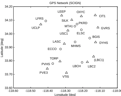
Figure 2. SCIGN stations used as reference stations (triangles) and ‘rover’ stations (circles)

GPS-Derived Tropospheric Delay Corrections

The Bernese GPS processing software (Rothacher & Mervart, 1996) was used to process the network on both days, the coordinates of CIT1 being held fixed as the primary reference station. Baseline lengths vary from 7km to 49km, and the largest height difference is 270m. For each site tropospheric delay corrections were determined every 20 minutes, resulting in six parameters per site throughout the 2-hour observation span. Single-differenced tropospheric corrections (equation (3)) were then obtained by forming the differences relative to CIT1. These corrections range from –6.1cm to +2.2cm, and in some cases show variations of a few centimeters within the 2-hour observation span.

change in the tropospheric conditions is of great importance. Hence double-differenced tropospheric corrections are obtained by forming the between-epoch difference of the single-differenced values derived in the previous step (equation (5)).

A comparison of the single- and double-differenced corrections revealed that almost all the double-differenced delay is smaller than the single-differenced delay (except for stations OXYC, MTA1 and PKRD). The double-differenced corrections range from –5.0cm to +3.3cm although the 23 stations spread over only a quarter of the SAR image frame (Figure 1). Therefore, it is crucial to apply such corrections in order for DInSAR to achieve sub-centimeter accuracy.

Interpolation of Tropospheric Delay Corrections

For each of the 9 ‘rover’ sites (prediction locations) shown in Figure 2, the tropospheric delay corrections were interpolated using the three methods described earlier: inverse distance weighted (IDW) interpolation, spline interpolation and kriging interpolation. Both the single-differenced tropospheric corrections relative to CIT1 for

days 214 and 249, and the double-differenced tropospheric corrections between these two epochs were investigated by comparing the interpolated values to the ‘true’ values obtained directly using the Bernese software. This was done for each of the six 20-minute time intervals within the 2-hour observation span.

As an example, Figure 3 shows the interpolation images obtained for the first time interval using the different interpolation methods in the double-differenced case, which is most important and can be directly used for the correction of differential InSAR results. The dots indicate the locations of the 22 GPS stations used in the analysis (refer to Figure 2 for their codes). The color/grey step interval is 1mm. The main areas of tropospheric activity can be recognized in all three images. Analysis of the images obtained for the following time intervals (not shown here) revealed the temporal and spatial variability of the tropospheric delay. The double-differenced interpolation values obtained with the different interpolation methods only differ by small amounts and are generally below or just above the cm-level. However, they can reach values of up to 3cm in some cases.

Figure 3. Double-differenced interpolation images for the first time interval using the (a) IDW, (b) spline and (c) kriging interpolation techniques

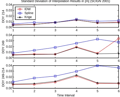
In order to determine which interpolation method gives the best results, the standard deviations of the results compared to the ‘true’ values obtained using the Bernese software were computed. Figure 4 shows the standard deviations for the single-differenced case on days 214 (top plot) and 249 (middle plot), as well as for the double-differenced case (bottom plot). It is obvious that all three interpolation techniques deliver results with the same accuracy in this particular case, which is mostly at the sub-centimeter level. For the fourth time interval the accuracy is considerably lower compared to the rest of the observation span, almost reaching the 2cm level. This may have been caused by a short-term tropospheric event on day 249, which again highlights the importance of

applying the differential tropospheric delay corrections to InSAR results.

Influence of Outliers in the GPS Reference Network on the Interpolation Results

site that had earlier been identified as having a problem, was now included as a reference station in the interpolation process. The data were then processed again. The standard deviations of the resulting tropospheric corrections for the single-differenced case on days 214 (top plot) and 249 (middle plot), as well as for the double-differenced case (bottom plot), are shown in Figure 5.

1 2 3 4 5 6

0.000 0.005 0.010 0.015 0.020 0.025

Standard Deviation of Interpolation Results in [m] (SCIGN 2001)

DOY 214

1 2 3 4 5 6

0.000 0.005 0.010 0.015 0.020 0.025

DOY 249

1 2 3 4 5 6

0.000 0.005 0.010 0.015 0.020 0.025

Time Interval

DOY 249-214

IDW Spline Krige

Figure 4. Standard deviation of the interpolation results obtained by different methods

1 2 3 4 5 6

0.00 0.01 0.02 0.03 0.04

Standard Deviation of Interpolation Results in [m] (SCIGN 2001)

DOY 214

1 2 3 4 5 6

0.00 0.01 0.02 0.03 0.04

DOY 249

1 2 3 4 5 6

0.00 0.01 0.02 0.03 0.04

Time Interval

DOY 249-214

IDW Spline Krige

Figure 5. Standard deviation of the interpolation results obtained by different methods (incl. outlier)

It is obvious that the spline interpolation method has difficulties coping with such an ‘outlier’ in the reference station network. Standard deviations reach values of up to 4cm in the double-differenced case. The values for the IDW and kriging interpolation techniques remain unchanged compared to the ‘clean’ reference network used in the previous study. Only the sixth time interval of the IDW interpolation on day 249 shows a change for the worse. However, this does not influence the double-differenced result (bottom graph of Figure 5), which indicates the robustness of the double-differencing algorithm proposed in this paper. It is therefore suggested that either the IDW or the kriging interpolation method be used to determine tropospheric delay parameters from

GPS observations. On the other hand, the two techniques can be used as checks on each other.

How Many Troposphere Parameters Should Be Determined?

The Bernese GPS processing software allows the user to specify the number of tropospheric delay parameters to be determined. Rothacher & Mervart (1996) recommend about 6-12 parameters for a 24-hour observation session. Estimating one parameter for every 2-4 hours may be sufficient for geodetic control surveys where a set of coordinates is derived from a long observation session, taking into account all possible atmospheric effects. However, a special situation arises when one is dealing with GPS-derived tropospheric corrections for InSAR. The SAR satellite will pass over the area of interest at a certain epoch and we are specifically interested in estimating the tropospheric delay as accurately as possible at this epoch within the observation span. It is therefore necessary to determine how many parameters should be estimated in order to obtain an accurate representation of the tropospheric conditions at any point in time.

A sub-network involving three GPS sites from the original network (Figure 2) was used. The baselines CIT1-UCLP and CIT1-VTIS are 30km and 49km in length with height differences of 104m and 156m respectively. The 2-hour session observed on September 6, 2001 (DOY 249) was processed several times incorporating a different number of estimable troposphere parameters. Tropospheric delay corrections were estimated for time intervals of 20, 10, 5 and 3 minutes in length, corresponding to 6, 12, 24 and 40 parameters per site respectively. Figure 6 shows the (single-differenced) tropospheric delay parameters for the sites UCLP (top) and VTIS (bottom), both relative to CIT1.

0 10 20 30 40 50 60 70 80 90 100 110 120 -0.020

-0.015 -0.010 -0.005 0.000 0.005 0.010

Relative Tropospheric Delay Parameters (UCLP)

Trop. Delay [m]

0 10 20 30 40 50 60 70 80 90 100 110 120 -0.020

-0.015 -0.010 -0.005 0.000 0.005 0.010

Relative Tropospheric Delay Parameters (VTIS)

Observation Time [min]

Trop. Delay [m]

20min 10min 5min 3min

Figure 6. Relative tropospheric delay parameters over 2 hours

and 20min cases produce a smoothed record of the tropospheric delay, which is obviously less likely to represent the correct conditions present at a specific SAR time epoch.

The resulting coordinates are practically the same for both the 3min and 5min tropospheric parameter estimation, with variations at the sub-mm level. If compared to the results obtained using 10min and 20min intervals, the coordinate differences are at the few-mm level. This corresponds to a difference of a few millimeters in the troposphere parameters between the 3min and 5min cases on the one hand and the 10min and 20min cases on the other (Figure 6).

These results indicate that by estimating tropospheric delay parameters for 5-minute time intervals during a 2-hour observation session, the short-term variations of the troposphere can be reliably modeled. At the same time the number of additional parameters to be estimated is still kept at a reasonable level.

EXPERIMENTAL DATA ANALYSIS: GEONET

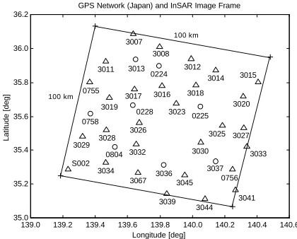
Based on the above findings a second data set from Japan’s GPS Earth Observation Network (GEONET) (GSI, 2003) was analyzed. Of the 37 stations considered, 29 were treated as measured locations (reference stations) and 8 were used as prediction locations (‘rover’ stations) for which tropospheric delay corrections had to be determined and compared with their GPS-derived delays. A 2-hour session was observed on June 17, 2002 (DOY 168) and on July 22, 2002 (DOY 203), again simulating a typical ERS SAR satellite single repeat cycle of 35 days, and covering the satellite flyover epoch. Figure 7 shows the location of the GPS sites, evenly distributed across a typical ERS SAR image frame (the dashed lines) for this area. The reference stations are denoted by triangles, while the sites to be interpolated are indicated by circles. Precise coordinates for all sites were provided by the Geographical Survey Institute (GSI) of Japan.

139.0 139.2 139.4 139.6 139.8 140.0 140.2 140.4 140.6 35.0

35.2 35.4 35.6 35.8 36.0 36.2

GPS Network (Japan) and InSAR Image Frame

Longitude [deg]

Latitude [deg]

100 km

100 km 3007

3011

3008 3013

0224 3012 ₃₀₁₄ 3018

3020 3015

0225 3023 3016 0755

3019 3017

0228 3026 0758

3029 3028 3032 0804 3034 S002

3067 3036 3045

3039 3044

3041 3033

0756 3037 3030

3025 3027

Figure 7. GEONET stations within the ERS SAR image

frame

GPS-Derived Tropospheric Delay Corrections

Again, the Bernese GPS processing software was used to process the network on both days, the coordinates of S002 being held fixed as the primary reference station. Baseline lengths vary from 22km to 121km, and the largest height difference is 321m. For each site tropospheric delay corrections were determined every 5 minutes, resulting in 24 parameters per site throughout the 2-hour observation span. It should be noted that in practice the primary reference station should be situated in, or close to, the center of the SAR image frame in order to keep the baseline lengths to a minimum. In this analysis, however, the results obtained over longer baselines are also of interest.

Single-differenced tropospheric corrections (equation (3)) were determined by forming the differences relative to S002. These corrections range from –9.5cm to +4.2cm, showing variations of up to a few centimeters within the 2-hour observation span.

The double-differenced tropospheric delay corrections were obtained by forming the between-epoch difference of the single-differenced values derived in the previous step (equation (5)). The double-differenced corrections range from –6.7cm to +10.9cm, indicating significant changes in the tropospheric conditions (see also Figure 8).

Interpolation of Tropospheric Delay Corrections

For each of the 8 ‘rover’ sites (prediction locations) shown in Figure 7, the tropospheric delay corrections were interpolated using the inverse distance weighted (IDW) interpolation method. Both the single-differenced tropospheric corrections relative to S002 for days 168 and 203, and the double-differenced tropospheric corrections between these two epochs were investigated by comparing the interpolated values to the ‘true’ values obtained directly using the Bernese software. This was done for each of the 24 5-minute time intervals within the 2-hour observation span.

Figure 8. Double-differenced interpolation maps for the 11th (left) and the 24th (right) time interval (IDW interpolation)

0 10 20 30 40 50 60 70 80 90 100 110 120 -0.10

-0.05 0.00 0.05 0.10 0.15

Double-Differenced Tropospheric Delay Parameters (0224, 85km)

Trop. Delay [m]

0 10 20 30 40 50 60 70 80 90 100 110 120 -0.10

-0.05 0.00 0.05 0.10

Double-Differenced Tropospheric Delay Parameters (0225, 85km)

Observation Time [min]

Trop. Delay [m]

Bernese interpolated difference

0 10 20 30 40 50 60 70 80 90 100 110 120 -0.10

-0.05 0.00 0.05 0.10

Double-Differenced Tropospheric Delay Parameters (0228, 55km)

Trop. Delay [m]

0 10 20 30 40 50 60 70 80 90 100 110 120 -0.10

-0.05 0.00 0.05 0.10

Double-Differenced Tropospheric Delay Parameters (0758, 38km)

Observation Time [min]

Trop. Delay [m]

0 10 20 30 40 50 60 70 80 90 100 110 120 -0.10

-0.05 0.00 0.05 0.10

Double-Differenced Tropospheric Delay Parameters (0804, 30km)

Trop. Delay [m]

0 10 20 30 40 50 60 70 80 90 100 110 120 -0.10

-0.05 0.00 0.05 0.10

Double-Differenced Tropospheric Delay Parameters (3013, 81km)

Observation Time [min]

Trop. Delay [m]

0 10 20 30 40 50 60 70 80 90 100 110 120 -0.10

-0.05 0.00 0.05 0.10

Double-Differenced Tropospheric Delay Parameters (3036, 54km)

Trop. Delay [m]

0 10 20 30 40 50 60 70 80 90 100 110 120 -0.10

-0.05 0.00 0.05 0.10

Double-Differenced Tropospheric Delay Parameters (3037, 83km)

Observation Time [min]

Trop. Delay [m]

Figure 9. Comparison of Benese-derived and interpolated double-differenced tropospheric corrections

Table 1. Standard deviations of the differences between Bernese-derived and interpolated troposphere corrections

Site STD [m] Baseline Length [km]

0224 0.00625 85

0225 0.00445 85

0228 0.00472 55

0758 0.00510 38

0804 0.00597 30

3013 0.01323 81

3036 0.00697 54

3037 0.00450 83

CONCLUDING REMARKS

Three interpolation methods, namely the inverse distance weighted, spline, and kriging techniques, have been investigated. Using GPS data from two test networks, it has been found that the inverse distance weighted and kriging interpolation methods are more suitable. Differential corrections as much as several centimeters may have to be applied in order to ensure sub-centimeter accuracy for the radar result. It seems optimal to estimate the tropospheric delay from GPS data at 5-minute intervals.

The algorithm and procedures developed in this paper could be easily implemented in a CGPS network data center. The interpolated grid of between-site, single-differenced tropospheric delays can be generated as a routine product to aid radar interferometry, in a manner similar to the SLC radar images.

ACKNOWLEDGMENTS

SCIGN and its sponsors, the W.M. Keck Foundation, NASA, NSF, USGS and SCEC, as well as Japan’s Geographical Survey Institute are thanked for providing the GPS data used in this study. The author is supported in his Ph.D. studies by an International Postgraduate Research Scholarship and funding from the Australian Research Council. The guidance and support provided by his supervisor Prof. Chris Rizos and Dr. Linlin Ge during this research are greatly appreciated. Mr. Yufei Wang is thanked for his assistance during the interpolation process.

REFERENCES

Bauersima, I. (1983): NAVSTAR/Global Positioning System (GPS) II: Radiointerferometrische Satelliten-beobachtungen, Mitteilungen der Satellitenbeobachtungs-station Zimmerwald, Bern, vol. 10.

Bock, Y. and S. Williams (1997): Integrated Satellite Interferometry in Southern California, EOS, 78(29), 293. de Boor, C. (1978): A Practical Guide to Splines, Springer, New York, 450pp.

Essen, L. and K.D. Froome (1951): The Refractive Indices and Dielectric Constants of Air and its Principal Constituents at 24000 Mc/s, Proc. of Physical Society, 64(B), 862-875.

Ge, L. (2000): Development and Testing of Augmentations of Continuously-Operating GPS Networks to Improve their Spatial and Temporal Resolution, The University of New South Wales, Australia, UNISURV S-63, 230pp. Ge, L., Y. Ishikawa, S. Fujiwara, S. Miyazaki, X. Qiao, X. Li, X. Yuan, W. Chen and J. Wang (1997): The Integration of InSAR and CGPS: A Solution to Efficient

Deformation Monitoring, Proc. Int. Symp. on Current

Crustal Movement & Hazard Reduction in East Asia and

South-East Asia, 4-7 November, Wuhan, P R. China, 145-155.

Graham, L.C. (1974): Synthetic Interferometer Radar for Topographic Mapping, Proc. IEEE, 62(6), 763-768. GSI (2003): http://mekira.gsi.go.jp/ENGLISH/index.html. Hanssen, R.F., T.M. Weckwerth, H.A. Zebker and R. Klees (1999): High-Resolution Water Vapor Mapping from Interferometric Radar Measurements, Science, 283, 1295-1297.

Lancaster, P. and K. Salkauskas (1986): Curve and

Surface Fitting: An Introduction, Academic Press,

London-Orlando, 280pp.

Lu, Z., R. Fatland, M. Wyss, S. Li, J. Eichelberger, K. Dean and J. Freymueller (1997): Deformation of New Trident Volcano Measured by ERS-1 SAR Interferometry,

Katmai National Park, Alaska, Geophysical Research

Letters, 24(6), 695-698.

Massonnet, D., M. Rossi, C. Carmona, F. Adragna, G. Peltzer, K. Feigl and T. Rabaute (1993): The Displacement Field of the Landers Earthquake Mapped by Radar Interferometry, Nature, 364, 138-142.

Mendes, V.B. (1999): Modeling the Neutral-Atmosphere

Propagation Delay in Radiometric Space Techniques,

PhD Dissertation, Dept. of Geodesy & Geomatics Eng. Tech. Rept. No. 199, University of New Brunswick, Fredericton, Canada, 353pp.

Rothacher, M. and L. Mervart (Eds.) (1996): Bernese GPS Software Version 4.0, Astronomical Institute, University of Berne, Switzerland, 418pp.

Saastamoinen, J. (1973): Contributions to the Theory of Atmospheric Refraction, Bulletin Géodésique, 107, 13-34.

Schultz, M.H. (1973): Spline Analysis, Prentice-Hall, Englewood Cliffs, N.J., 156pp.

SCIGN (2003): http://www.scign.org/.

SOPAC (2003): http://sopac.ucsd.edu/cgi-bin/SCOUT.cgi. Spilker, J.J. (1996): Tropospheric Effects on GPS, in: Parkinson, B.W. and J.J. Spilker (Eds.) (1996): Global

Positioning System: Theory and Applications Volume 1,

Progress in Astronautics and Aeronautics, 163, American Institute of Aeronautics and Astronautics, Washington, 517-546.