A randomised method for the shapely value for the voting game

A Randomized Method for the Shapley Value

for the Voting Game

Shaheen S. Fatima

Department of Computer Science, University of Liverpool Liverpool L69 3BX, UK.

[email protected]

Michael Wooldridge

Department of Computer Science, University of Liverpool Liverpool L69 3BX, UK.

[email protected]

Nicholas R. Jennings

School of Electronics and

Computer Science University of Southampton Southampton SO17 1BJ, UK.

[email protected]

ABSTRACT

The Shapley value is one of the key solution concepts for coali-tion games. Its main advantage is that it provides a unique and fair solution, but its main problem is that, for many coalition games, the Shapley value cannot be determined in polynomial time. In particular, the problem of finding this value for the voting game is known to be #P-complete in the general case. However, in this pa-per, we show that there are some specific voting games for which the problem is computationally tractable. For other general voting games, we overcome the problem of computational complexity by presenting a new randomized method for determining the

approxi-mate Shapley value. The time complexity of this method is linear

in the number of players. We also show, through empirical studies, that the percentage error for the proposed method is always less than 20% and, in most cases, less than 5%.

Categories and Subject Descriptors

I.2.11 [Distributed Artificial Intelligence]: Multiagent Systems

General Terms

Algorithms, Design, Theory

Keywords

Game-theory, Coalition Formation, Approximation, Shapley Value.

1.

INTRODUCTION

Coalition formation, a key form of interaction in multi-agent sys-tems, is the process of joining together two or more agents so as to achieve goals that individuals on their own cannot, or to achieve them more efficiently [1, 11, 14, 13]. Often, in such situations, there is more than one possible coalition and a player’s payoff de-pends on which one it joins. Given this, a key problem is to ensure that none of the parties in a coalition has any incentive to break away from it and join another coalition (i.e., the coalitions should be stable). However, in many cases there may be more than one

Permission to make digital or hard copies of all or part of this work for personal or classroom use is granted without fee provided that copies are not made or distributed for profit or commercial advantage and that copies bear this notice and the full citation on the first page. To copy otherwise, to republish, to post on servers or to redistribute to lists, requires prior specific permission and/or a fee.

AAMAS’07 May 14–18 2007, Honolulu, Hawai’i, USA. Copyright 2007 IFAAMAS .

solution (i.e., a stable coalition). In such cases, it becomes difficult to select a single solution from among the possible ones, especially if the parties are self-interested (i.e., they have different preferences over stable coalitions).

In this context, cooperative game theory deals with the prob-lem of coalition formation and offers a number of solution con-cepts that possess desirable properties like stability, fair division

of joint gains, and uniqueness [16, 14]. Cooperative game theory

differs from its non-cooperative counterpart in that for the former the players are allowed to form binding agreements and so there is a strong incentive to work together to receive the largest total pay-off. Also, unlike non-cooperative game theory, cooperative game theory does not specify a game through a description of the strate-gic environment (including the order of players’ moves and the set of actions at each move) and the resulting payoffs, but, instead, it reduces this collection of data to the coalitional form where each coalition is represented by a single real number: there are no ac-tions, moves, or individual payoffs. The chief advantage of this approach, at least in multiple-player environments, is its practical usefulness. Thus, many more real-life situations fit more easily into a coalitional form game, whose structure is more tractable than that of a non-cooperative game, whether that be in normal or extensive form and it is for this reason that we focus on such forms in this paper.

Given these observations, a number of multiagent systems re-searchers have used and extended cooperative game-theoretic solu-tions to facilitate automated coalition formation [20, 21, 18]. More-over, in this work, one of the most extensively studied solution con-cepts is the Shapley value [19]. A player’s Shapley value gives an indication of its prospects of playing the game – the higher the Shapley value, the better its prospects. The main advantage of the Shapley value is that it provides a solution that is both unique and

fair (see Section 2.1 for a discussion of the property of fairness).

be computed in polynomial time. By identifying such games, we show, for the first tme, when it is feasible to find the exact value and when it is not. For the computationally complex voting games, we present a new randomised method, along the lines of Monte-Carlo

simulation, for computing the approximate Shapley value.

The computational complexity of such games has typically been tackled using two main approaches. The first is to use

generat-ing functions [3]. This method trades time complexity for

stor-age space. The second uses an approximation technique based on

Monte Carlo simulation [12, 7]. However the method we propose is

more general than either of these (see Section 6 for details). More-over, no work has previously analysed the approximation error. The approximation error relates to how close the approximate is to the true Shapley value. Specifically, it is the difference between the true and the approximate Shapley value. It is important to determine this error because the performance of an approximation method is evaluated in terms of two criteria: its time complexity, and its ap-proximation error. Thus, our contribution lies in also in providing, for the first time, an analysis of the percentage error in the approx-imate Shapley value. This analysis is carried out empirically.

Our experiments show that the error is always less than 20%, and in most cases it is under 5%. Finally, our method has time complexity linear in the number of players and it does not require any arrays (i.e., it is economical in terms of both computing time and storage space). Given this, and the fact that software agents have limited computational resources and therefore cannot com-pute the true Shapley value, our results are especially relevant to such resource bounded agents.

The rest of the paper is organised as follows. Section 2 defines the Shapley value and describes the weighted voting game. In Sec-tion 3 we describe voting games whose Shapley value can be found in polynomial time. In Section 4, we present a randomized method for finding the approximate Shapley value and analyse its perfor-mance in Section 5. Section 6 discusses related literature. Finally, Section 7 concludes.

2.

BACKGROUND

We begin by introducing coalition games and the Shapley value and then define the weighted voting game. A coalition game is a game where groups of players (“coalitions”) may enforce cooperative be-haviour between their members. Hence the game is a competition between coalitions of players, rather than between individual play-ers.

Depending on how the players measure utility, coalition game theory is split into two parts. If the players measure utility or the payoff in the same units and there is a means of exchange of utility such as side payments, we say the game has transferable utility; otherwise it has non-transferable utility. More formally, a coalition game with transferable utility,_hN, vi, consists of:

1. a finite set (N =_{1,2, . . . , n_}) of players and

2. a function (v) that associates with every non-empty subsetS

ofN(i.e., a coalition) a real numberv(S)(the worth ofS).

For each coalitionS, the numberv(S)is the total payoff that is available for division among the members ofS(i.e., the set of joint actions that coalitionS can take consists of all possible divisions ofv(S)among the members of S). Coalition games with non-transferable payoffs differ from ones with non-transferable payoffs in the following way. For the former, each coalition is associated with a set of payoff vectors that is not necessarily the set of all possible divisions of some fixed amount. The focus of this paper is on the

weighted voting game (described in Section 2.1) which is a game with transferable payoffs.

Thus, in either case, the players will only join a coalition if they expect to gain from it. Here, the players are allowed to form bind-ing agreements, and so there is strong incentive to work together to receive the largest total payoff. The problem then is how to split the total payoff between or among the players. In this context, Shapley [19] constructed a solution using an axiomatic approach. Shapley defined a value for games to be a function that assigns to a game (N, v), a numberϕi(N, v)for eachiinN. This function satisfies three axioms [17]:

1. Symmetry. This axiom requires that the names of players play no role in determining the value.

2. Carrier. This axiom requires that the sum ofϕi(N, v)for all playersiin any carrierCequalv(C). A carrierCis a subset ofN such thatv(S) =v(S∩C)for any subset of players

S_⊂N.

3. Additivity. This axiom specifies how the values of different games must be related to one another. It requires that for any gamesϕi(N, v)andϕi(N, v0),ϕi(N, v)+ϕi(N, v0) =

ϕi(N, v+v0_{)for alliinN.}

Shapley showed that there is a unique function that satisfies these three axioms.

Shapley viewed this value as an index for measuring the power of players in a game. Like a price index or other market indices, the value uses averages (or weighted averages in some of its generaliza-tions) to aggregate the power of players in their various cooperation opportunities. Alternatively, one can think of the Shapley value as a measure of the utility of risk neutral players in a game.

We first introduce some notation and then define the Shapley value. Let_S denote the setN _{− {}i_}and fi : _{S →} 2N−{i}_be

a random variable that takes its values in the set of all subsets of

N_{− {}i_}, and has the probability distribution function (g) defined as:

g(fi(S) =S) = |S|!(n− |S| −1)!

n!

The random variablefiis interpreted as the random choice of a coalition that playerijoins. Then, a player’s Shapley value is de-fined in terms of its marginal contribution. Thus, the marginal con-tribution of playerito coalitionSwithi /∈Sis a function∆ivthat is defined as follows:

∆iv(S) =v(S_{∪ {}i_})₋v(S)

Thus a player’s marginal contribution to a coalition S is the in-crease in the value ofSas a result ofijoining it.

DEFINITION 1. The Shapley value (ϕi) of the game_hN, v_ifor player iis the expectation (E) of its marginal contribution to a coalition that is chosen randomly:

ϕi(N, v) =E[∆iv_◦fi] (1)

The Shapley value is interpreted as follows. Suppose that all the players are arranged in some order, all orderings being equally likely. Thenϕi(N, v)is the expected marginal contribution, over all orderings, of playerito the set of players who precede him.

The method for finding a player’s Shapley value depends on the definition of the value function (v). This function is different for different games, but here we focus specifically on the weighted

2.1

The weighted voting game

We adopt the definition of the voting game given in [6]. Thus, there is a set ofnplayers that may, for example, represent shareholders in a company or members in a parliament. The weighted voting game is then a gameG=_hN, v_iin which:

v(S) =



1 ifw(S)≥q

0 otherwise

for someq_∈IR+andwi∈IRN+, where:

w(S) = X

i∈S wi

for any coalitionS. Thuswiis the number of votes that playeri

has andqis the number of votes needed to win the game (i.e., the

quota).

Note that for this game (denoted _hq;w1, . . . , wni), a player’s

marginal contribution is either zero or one. This is because the value of any coalition is either zero or one. A coalition with value zero is called a “losing coalition” and with value one a “winning coalition”. If a player’s entry to a coalition changes it from losing to winning, then the player’s marginal contribution for that coalition is one; otherwise it is zero.

The main advantage of the Shapley value is that it gives a so-lution that is both unique and fair. The property of uniqueness is desirable because it leaves no ambiguity. The property of fair-ness relates to how the gains from cooperation are split between the members of a coalition. In this case, a player’s Shapley value is proportional to the contribution it makes as a member of a coali-tion; the more contribution it makes, the higher its value. Thus, from a player’s perspective, both uniqueness and fairness are desir-able properties.

3.

VOTING GAMES WITH POLYNOMIAL

TIME SOLUTIONS

Here we describe those voting games for which the Shapley value can be determined in polynomial time. This is achieved using the direct enumeration approach (i.e., listing all possible coalitions and finding a player’s marginal contribution to each of them). We char-acterise such games in terms of the number of players and their weights.

3.1

All players have equal weight

Consider the gamehq;j, . . . , jiwithmparties. Each party hasj

votes. Ifq_≤j, then there would be no need for the players to form a coalition. On the other hand, ifq=mj(m=_|N_|is the number of players), only the grand coalition is possible. The interesting games are those for which the quota (q) satisfies the constraint: (j+ 1)_≤q_≤j(m₋1). For these games, the value of a coalition is one if the weight of the coalition is greater than or equal toq, otherwise it is zero.

Letϕdenote the Shapley value for a player. Consider any one player. This player can join a coalition as theith member where 1≤i≤m. However, the marginal contribution of the player is1 only if it joins a coalition as the_dq/j_eth member. In all other cases, its marginal contribution is zero. Thus, the Shapley value for each playerϕ = 1/m. Sinceϕrequires one division operation, it can be found in constant time (i.e.,_O(1)).

3.2

A single large party

Consider a game in which there are two types of players: large (with weightwl > ws) and small (with weightws). There is one large player andmsmall ones. The quota for this game isq; i.e., we

have a game of the form_hq;wl, ws, ws, . . . , ws_i. The total number of players is(m+ 1). The value of a coalition is one if the weight of the coalition is greater than or equal toq, otherwise it is zero. Letϕldenote the Shapley value for the large player andϕsthat for each small player.

We first considerws = 1and thenws >1. The smallest pos-sible value forqiswl+ 1. This is because, ifq ≤wl, then the large party can win the election on its own without the need for a coalition. Thus, the quota for the game satisfies the constraint

wl+ 1≤q ≤m+wl−1. Also, the lower and upper limits for

wlare2and(q₋1)respectively. The lower limit is2because the weight of the large party has to be greater than each small one. Furthermore, the weight of the large party cannot be greater than

q, since in that case, there would be no need for the large party to form a coalition. Recall that for our voting game, a player’s marginal contribution to a coalition can only be zero or one.

Consider the large party. This party can join a coalition as the

ith member where1 _≤ i _≤ (m+ 1). However, the marginal contribution of the large party is one if it joins a coalition as the

ith member where(q−wl) ≤i < q. In all the remaining cases, its marginal contribution is zero. Thus, out of the total(m+ 1) possible cases, its marginal contribution is one inwlcases. Hence, the Shapley value of the large party is: ϕl=wl/(m+ 1). In the same way, we obtain the Shapley value of the large party for the general case wherews>1as:

ϕl = _dwl/ws_e/(m+ 1)

Now consider a small player. We know that the sum of the Shap-ley values of all them+ 1players is one. Also, since the small par-ties have equal weights, their Shapley values are the same. Hence, we get:

ϕs = 1−ϕl

m

Thus, bothϕlandϕscan be computed in constant time. This is because both require a constant number of basic operations (ad-dition, subtraction, multiplication, and division). In the same way, the Shapley value for a voting game with a single large party and multiple small parties can be determined in constant time.

3.3

Multiple large and small parties

We now consider a voting game that has two player types: large and small (as in Section 3.2), but now there are multiple large and multiple small parties. The set of parties consists ofmllarge par-ties andmssmall parties. The weight of each large party iswland that of each small one isws, wherews< wl. We show the compu-tational tractability for this game by considering the following four possible scenarios:

S1 q≤mlwlandq≤msws

S2 q≤mlwlandq≥msws

S3 q≥mlwlandq≥msws

S4 q≥mlwlandq≤msws

Consider a coalition such that when the large player joins in, there areilarge players and(q₋iwl₋1)/wssmall players al-ready in it, and the remaining players join after the large player. Such a coalition gives the large player unit marginal contribution. Let_Cl2(i, q)denote the number of all such coalitions. To begin, consider the casei= 0:

C2l(0, q) = C

„

ms,q−1

ws

«

×FACTORIAL

„

q−1

ws

«

×

FACTORIAL

„

ml+ms−q_ws−1−1

«

whereC(y, x)denotes the number of possible combinations ofx

items from a set ofyitems. Fori= 1, we get:

C2l(1, q) = C(ml,1)×C

„

ms,q−wl−1

ws

«

×

FACTORIAL

„

q−wl−1

ws

«

×

FACTORIAL

„

ml+ms−q−_wswl−1−1

«

In general, fori >1, we get:

Cl2(i, q) =C(ml, i)×C

„

ms,q−iwl−1

ws

«

×

FACTORIAL

„

q₋iwl₋1

ws

«

×

FACTORIAL

„

ml+ms₋q−wl−1

ws −1

«

Thus the large player’s Shapley value is:

ϕl =

q−1

wl

X

i=0

C2l(i, q)/FACTORIAL(ml+ms)

For a giveni, the time to find_Cl2(i, q)is_O(T)where

T = (mlms(q−iwl−1)(ml+ms))/ws

Hence, the time to find the Shapley value is_O(T q/wl). In the same way, a small player’s Shapley value is:

ϕs =

q−1

ws

X

i=0 C2

s(i, q)/FACTORIAL(ml+ms)

and can be found in time_O(T q/ws). Likewise, the remaining three scenarios (S2toS4) can be shown to have the same time

complex-ity.

3.4

Three player types

We now consider a voting game that has three player types:1,2, and3. The set of parties consists ofm1 players of type 1(each

with weightw1),m2players of type2(each with weightw2), and

m3players of type3(each with weightw3).

For this voting game, consider a player of type1. It is possible for the marginal contribution of this player to be one if it joins a coalition in which the number of type1players is between zero and(q₋1)/w1. In other words, there are(q−1)/w1+ 1such

cases and we now consider each of them.

Consider a coalition such that when the type1player joins in, there areitype1players already in it. The remaining players join after the type1player. Let_Cl3(i, q)denote the number of all such

coalitions that give a marginal contribution of one to the type 1 player where:

C13(i, q) = q−1

w1

X

i=0 q−iw1−1

w2

X

j=0

C12(j, q−iw1)

Therefore the Shapley value of the type1player is:

ϕ1 =

q−1

w1

X

i=0 C3

1(i, q)/FACTORIAL(m1+m2+m3)

The time complexity of finding this value isO(T q2/w1w2)where:

T = (

3

Y

i=1

mi)(q₋iwl₋1)(

3

X

i=1

mi)/(w2+w3)

Likewise, for the other two player types (2and3).

Thus, we have identified games for which the exact Shapley value can be easily determined. However, the computational com-plexity of the above direct enumeration method increases with the number of player types. For a voting game with more than three player types, the time complexity of the above method is a polyno-mial of degree four or more. To deal with such situations, therefore, the following section presents a faster randomised method for find-ing the approximate Shapley value.

4.

FINDING THE APPROXIMATE SHAPLEY

VALUE

We first give a brief introduction to randomized algorithms and then present our randomized method for finding the approximate Shapley value. Randomized algorithms are the most commonly used approach for finding approximate solutions to computation-ally hard problems. A randomized algorithm is an algorithm that, during some of its steps, performs random choices [2]. The ran-dom steps performed by the algorithm imply that by executing the algorithm several times with the same input we are not guaranteed to find the same solution. Now, since such algorithms generate ap-proximate solutions, their performance is evaluated in terms of two criteria: their time complexity, and their error of approximation. The approximation error refers to the difference between the ex-act solution and its approximation. Against this background, we present a randomized method for finding the approximate Shapley value and empirically evaluate its error.

We first describe the general voting game and then present our randomized algorithm. In its general form, a voting game has more than two types of players. Let wi denote the weight of player

i. Thus, form players and for quotaq the game is of the form

hq;w1, w2, . . . , wmi. The weights are specified in terms of a

prob-ability distribution function. For such a game, we want to find the approximate Shapley value.

We letP denote a population of players. The players’ weights in this population are defined by a probability distribution function. Irrespective of the actual probability distribution function, letµbe the mean weight for the population of players andνthe variance in the players’ weights. From this population of players we randomly draw samples and find the sum of the players’ weights in the sample using the following rule from Sampling Theory (see [8] p425):

Ifw1, w2, . . . , wnis a random sample of sizendrawn

from any distribution with meanµand varianceν, then the sample sum has an approximate Normal

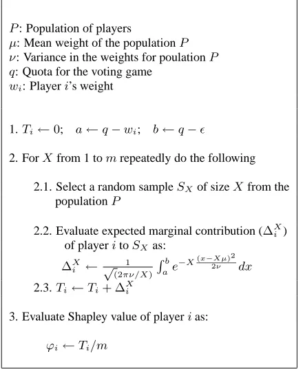
R-SHAPLEYVALUE(P, µ, ν, q, wi)

P: Population of players

µ: Mean weight of the populationP ν: Variance in the weights for poulationP q: Quota for the voting game

wi: Playeri’s weight

1.Ti_←0; a_←q₋wi; b_←q₋

2. ForXfrom 1 tomrepeatedly do the following

2.1. Select a random sampleSXof sizeXfrom the populationP

2.2. Evaluate expected marginal contribution (∆Xi )

of playeritoSXas:

∆X

i ← √_(2πν/X1 ₎

Rb

ae

−X(x−Xµ)2

2ν dx

2.3.Ti_←Ti+ ∆X i

3. Evaluate Shapley value of playerias:

[image:5.612.65.285.30.298.2]

ϕi_←Ti/m

Table 1: Randomized algorithm to find the Shapley value for playeri.

We know from Definition 1, that the Shapley value for a player is the expectation (E) of its marginal contribution to a coalition that is chosen randomly. We use this rule to determine the Shapley value as follows.

For playeriwith weightwi, letϕidenote the Shapley value. Let

X denote the size of a random sample drawn from a population in which the individual player weights have any distribution. The marginal contribution of playerito this random sample is one if the total weight of theXplayers in the sample is greater than or equal toa=q₋wibut less thanb=q₋(whereis an inifinitesimally small quantity). Otherwise, its marginal contribution is zero. Thus, the expected marginal contribution of playeri(denoted∆X

i ) to the

sample coalition is the area under the curve defined by_N(Xµ, ν X)

in the interval[a, b]. This area is shown as the regionBin Figure 1 (the dotted line in the figure isXµ). Hence we get:

∆Xi =

1

p

(2πν/X)

Zb

a

e−X(x−2Xµν )2_{dx (2)}

and the Shapley value is:

ϕi = 1

m m

X

X=1

∆Xi (3)

The above steps are described in Table 1. In more detail, Step 1 does the initialization. In Step 2, we varyX between 1 andm

and repeatedly do the following. In Step 2.1, we randomly select a sampleSX of sizeX from the populationP. Playeri’s marginal contribution to the random coalitionSXis found in Step 2.2. The average marginal contribution is found in Step 3 – and this is the Shapley value for playeri.

THEOREM 1. The time complexity of the proposed randomized

method is linear in the number of players.

PROOF. As per Equation 3,∆X

i must be computedmtimes.

This is done in the for loop of Step 2 in Table 1. Hence, the time complexity of computing a player’s Shapley value isO(m).

The following section analyses the approximation error for the pro-posed method.

5.

PERFORMANCE OF THE RANDOMIZED

METHOD

We first derive the formula for measuring the error in the approx-imate Shapley value and then conduct experiments for evaluating this error in a wide range of settings. However, before doing so, we introduce the idea of error.

The concept of error relates to a measurement made of a quan-tity which has an accepted value [22, 4]. Obviously, it cannot be determined exactly how far off a measurement is from the accepted value; if this could be done, it would be possible to just give a more accurate, corrected value. Thus, error has to do with uncertainty in measurements that nothing can be done about. If a measurement is repeated, the values obtained will differ and none of the results can be preferred over the others. However, although it is not possible to do anything about such error, it can be characterized.

As described in Section 4, we make measurements on samples that are drawn randomly from a given population (P) of players. Now, there are statistical errors associated with sampling which are unavoidable and must be lived with. Hence, if the result of a measurement is to have meaning it cannot consist of the measured value alone. An indication of how “accurate” the result is must be included also. Thus, the result of any physical measurement has two essential components:

1. a numerical value giving the best “estimate” possible of the quantity measured, and

2. the degree of uncertainty associated with this estimated value.

For example, if the estimate of a quantity isxand the uncertainty ise(x)the quantity would lie inx_±e(x).

For sampling experiments, the standard error is by far the most common way of characterising uncertainty [22]. Given this, the following section defines this error and uses it to evaluate the per-formance of the proposed randomized method.

5.1

Approximation error

The accuracy of the above randomized method depends on its sam-pling error which is defined as follows [22, 4]:

DEFINITION 2. The sampling error (or standard error) is

de-fined as the standard deviation for a set of measurements divided by the square root of the number of measurements.

To this end, lete(σX_{)be the sampling error in the sum of the}

weights for a sample of sizeXdrawn from the distribution_N(Xµ,_Xν) where:

e(σX) = p

(ν/X)/p

(X)

b

C

B

a − e(σX) a

A

) X (σ

e

b+ Sum of weights

[image:6.612.343.533.20.168.2]

Z1 Z2

Figure 1: A normal distribution for the sum of players’ weights in a coalition of sizeX.

40 60

80

100 0

50

100 0

5 10 15 20 25

Quota Weight

[image:6.612.77.272.169.322.2]

Percentage error in the Shapley value

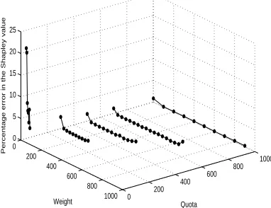
Figure 2: Performance of the randomized method form= 10

players.

coalition of sizeX. Since the error in this sum ise(σX_{), the actual}

values ofaand blie in the intervala_±e(σX_{)and b}

±e(σX₎

respectively. Hence, the error in Equation 2 is either the probability that the sum lies between the limitsa−e(σX)anda(i.e., the area under the curve defined by_N(Xµ, ν

X)betweena−e(σ

X_)anda,

which is the shaded regionAin Figure 1) or the probability that the sum of weights lies between the limitsbandb+e(σX)(i.e., the area under the curve defined by_N(Xµ, ν

X)betweenbandb+e(σ X_),

which is the shaded regionCin Figure 1). More specifically, the error is the maximum of these two probabilities:

e(∆Xi ) =

1

p

(2πν/X)×MAX

„Z a a−e(σX₎

e−X(x−2Xµν )2dx,

Z b+e(σX₎

b

e−X(x−2Xµν )2_dx

«

On the basis of the above error, we find the error in the Shapley value by using the following standard error propagation rules [22]:

R1 Ifxandyare two random variables with errorse(x)ande(y) respectively, then the error in the random variablez=x+y

is given by:

e(z) = e(x) +e(y)

R2 Ifxis a random variable with errore(x)andz=kxwhere

0 100

200 300

400 500 0

100 200

300 400

500 0

5 10 15 20 25

Quota Weight

Percentage error in the Shapley value

Figure 3: Performance of the randomized method form= 50

players.

the constantkhas no error, then the error inzis:

e(z) = _|k_|e(x)

Using the above rules, the error in the Shapley value (given in Equation 3) is obtained by propagating the error in Equation 4 to all coalitions between the sizesX = 1andX = m. Lete(ϕi) denote this error where:

e(ϕi) = 1

m m

X

X=1

e(∆Xi )

We analyze the performance of our method in terms of the per-centage errorPEin the approximate Shapley value which is defined as follows:

PE = 100×e(ϕi)/ϕi (5)

5.2

Experimental Results

We now compute the percentage error in the Shapley value using the above equation forPE. Since this error depends on the param-eters of the voting game, we evaluate it in a range of settings by systematically varying the parameters of the voting game.

In particular, we conduct experiments in the following setting. For a player with weightw, the percentage error in a player’s Shap-ley value depends on the following five parameters (see Equation 3):

1. The number of parties (m).

2. The mean weight (µ).

3. The variance in the player’s weights (ν).

4. The quota for the voting game (q).

5. The given player’s weight (w).

We fixµ = 10 andν = 1. This is because, for the normal distribution, µ = 10ensures that for almost all the players the weight is positive, andν= 1is used most commonly in statistical experiments (νcan be higher or lower butPEis increasing inν– see Equations 4 and 5). We then varym,q, andwas follows. We varymbetween 5 and 100 (since beyond 100 we found that the error is close to zero), for eachmwe varyqbetween4µandmµ

[image:6.612.57.290.502.556.2]

0 200

400 600

800 1000 0

200 400

600 800

1000 0

5 10 15 20 25

Quota Weight

[image:7.612.80.271.21.168.2]

Percentage error in the Shapley value

Figure 4: Performance of the randomized method form= 100

players.

winning coalition is more than one and less thanm– see Section 3 for details), and for eachq, we varywbetween1andq−1(because a winning coalition must contain at least two players). The results of these experiments are shown in Figures 2, 3, and 4. As seen in the figures, the maximumPEis around 20% and in most cases it is below 5%.

We now analyse the effect of the three parameters:w,q, andm

on the percentage error in more detail.

- Effect ofw. ThePEdepends one(σX)because, in Equa-tion 5, the limits of integraEqua-tion depend one(σX). The inter-val over which the first integration in Equation 5 is done is

a−a+e(σX_{) = e(σ}X_{), and the interval over which the}

second one is done isb+e(σX)−b=e(σX). Thus, the in-terval is the same for both integrations and it is independent ofwi. Note that each of the two functions that are integrated in Equation 5 are the same as the function that is integrated in Equation 2. Only the limits of the integration are different. Also, the interval over which the integration for the marginal contribution of Equation 2 is done isb−a = wi−(see Figure 1). The error in the marginal contribution is either the area of the shaded regionA(betweena₋e(σX_{)anda) in}

Figure 1, or the shaded areaC(betweenbandb+e(σX)). As per Equation 5, it is the maximum of these two areas. Sincee(σX_{)is independent ofwi, aswiincreases,e(σ}X₎

remains unchanged. However, the area of the unshaded re-gionB increases. Hence, aswi increases, the error in the marginal contribution decreases andPEalso decreases.

- Effect ofq. For a givenq, the Shapley value for playeriis as given in Equation 3. We know that, for a sample of size

X, the sum of the players’ weights is distributed normally with meanXµand varianceν/X. Since 99% of a normal distribution lies within two standard deviations of its mean [8], playeri’s marginal contribution to a sample of sizeXis almost zero if:

a < Xµ+ 2p

ν/X or b > Xµ₋2p

ν/X

This is because the three regionsA,B, andC(in Figure 1) lie either to the right ofZ2or to the left ofZ1. However, playeri’s marginal contribution is greater than zero for those

Xfor which the following constraint is satisfied:

Xµ−2pν/X < a < b < Xµ+ 2pν/X

For this constraint, the three regionsA,B, andClie some-where betweenZ1andZ2. Sincea=q₋wiandb=q₋, Equation 6 can also be written as:

Xµ₋2pν/X < q₋wi< q₋ < Xµ+ 2pν/X

The smallestX that satisfies the constraint in Equation 6 strictly increases withq. AsX increases, the error in sum of weights in a sample (i.e.,e(σX) =p

(ν)/X) decreases. Consequently, the error in a player’s marginal contribution (see Equation 5) also decreases. This implies that asq in-creases, the error in the marginal contribution (and conse-quently the error in the Shapley value) decreases.

- Effect ofm. It is clear from Equation 4 that the errore(σX) is highest forX = 1and it decreases withX. Hence, for smallm,e(σ1_{)has a significant effect on}

PE. But asm in-creases, the effect ofe(σ1)onPEdecreases and, as a result,

PEdecreases.

6.

RELATED WORK

In order to overcome the computational complexity of finding the Shapley value, two main approaches have been proposed in the literature. One approach is to use generating functions [3]. This method is an exact procedure that overcomes the problem of time complexity, but its storage requirements are substantial – it requires huge arrays. It also has the limitation (not shared by other ap-proaches) that it can only be applied to games with integer weights and quotas.

The other method uses an approximation technique based on

Monte Carlo simulation. In [12], for instance, the Shapley value is

computed by considering a random sample from a large population of players. The method we propose differs from this in that they de-fine the Shapley value by treating a player’s number of swings (if a player can change a losing coalition to a winning one, then, for the player, the coalition is counted as a swing) as a random variable, while we treat the players’ weights as random variables. In [12], however, the question remains how to get the number of swings from the definition of a voting game and what is the time complex-ity of doing this. Since the voting game is defined in terms of the players’ weights and the number of swings are obtained from these weights, our method corresponds more closely to the definition of the voting game. Our method also differs from [7] in that while [7] presents a method for the case where all the players’ weights are distributed normally, our method applies to any type of distribution for these weights. Thus, as stated in Section 1, our method is more general than [3, 12, 7]. Also, unlike all the above mentioned work, we provide an analysis of the performance of our method in terms of the percentage error in the approximate Shapley value.

of the representation and gives an approximate Shapley value in linear time, without the need for an oracle.

7.

CONCLUSIONS AND FUTURE WORK

Coalition formation is an important form of interaction in multi-agent systems. An important issue in such work is for the multi-agents to decide how to split the gains from cooperation between the mem-bers of a coalition. In this context, cooperative game theory offers a solution concept called the Shapley value. The main advantage of the Shapley value is that it provides a solution that is both unique and fair. However, its main problem is that, for many coalition games, the Shapley value cannot be determined in polynomial time. In particular, the problem of finding this value for the voting game is #P-complete. Although this problem is, in general #P-complete, we show that there are some specific voting games for which the Shapley value can be determined in polynomial time and charac-terise such games. By doing so, we have shown when it is computa-tionally feasible to find the exact Shapley value. For other complex voting games, we presented a new randomized method for deter-mining the approximate Shapley value. The time complexity of the proposed method is linear in the number of players. We analysed the performance of this method in terms of the percentage error in the approximate Shapley value.

Our experiments show that the percentage error in the Shapley value is at most 20. Furthermore, in most cases, the error is less than 5%. Finally, we analyse the effect of the different parameters of the voting game on this error. Our study shows that the error decreases as

1. a player’s weight increases,

2. the quota increases, and

3. the number of players increases.

Given the fact that software agents have limited computational re-sources and therefore cannot compute the true Shapley value, our results are especially relevant to such resource bounded agents. In future, we will explore the problem of determining the Shapley value for other commonly occurring coalition games like the “pro-duction economy” and the “market economy”.

8.

REFERENCES

[1] R. Aumann. Acceptable points in general cooperative n-person games. In Contributions to theTheory of Games

volume IV. Princeton University Press, 1959.

[2] G. Ausiello, P. Crescenzi, G. Gambosi, V. Kann,

A. Marchetti-Spaccamela, and M. Protasi. Complexity and

approximation: Combinatorial optimization problems and their approximability properties. Springer, 2003.

[3] J. M. Bilbao, J. R. Fernandez, A. J. Losada, and J. J. Lopez. Generating functions for computing power indices efficiently. Top 8, 2:191–213, 2000.

[4] P. Bork, H. Grote, D. Notz, and M. Regler. Data Analysis

Techniques in High Energy Physics Experiments. Cambridge

University Press, 1993.

[5] V. Conitzer and T. Sandholm. Computing Shapley values, manipulating value division schemes, and checking core membership in multi-issue domains. In Proceedings of the

National Conference on Artificial Intelligence, pages

219–225, San Jose, California, 2004.

[6] X. Deng and C. H. Papadimitriou. On the complexity of cooperative solution concepts. Mathematics of Operations

Research, 19(2):257–266, 1994.

[7] S. S. Fatima, M. Wooldridge, and N. R. Jennings. An analysis of the shapley value and its uncertainty for the voting game. In Proc. 7th Int. Workshop on Agent Mediated

Electronic Commerce, pages 39–52, 2005.

[8] A. Francis. Advanced Level Statistics. Stanley Thornes Publishers, 1979.

[9] S. Ieong and Y. Shoham. Marginal contribution nets: A compact representation scheme for coalitional games. In

Proceedings of the Sixth ACM Conference on Electronic Commerce, pages 193–202, Vancouver, Canada, 2005.

[10] S. Ieong and Y. Shoham. Multi-attribute coalition games. In

Proceedings of the Seventh ACM Conference on Electronic Commerce, pages 170–179, Ann Arbor, Michigan, 2006.

[11] J. P. Kahan and A. Rapoport. Theories of Coalition

Formation. Lawrence Erlbaum Associates Publishers, 1984.

[12] I. Mann and L. S. Shapley. Values for large games iv: Evaluating the electoral college exactly. Technical report, The RAND Corporation, Santa Monica, 1962.

[13] A. MasColell, M. Whinston, and J. R. Green.

Microeconomic Theory. Oxford University Press, 1995.

[14] M. J. Osborne and A. Rubinstein. A Course in Game Theory. The MIT Press, 1994.

[15] C. H. Papadimitriou. Computational Complexity. Addison Wesley Longman, 1994.

[16] A. Rapoport. N-person Game Theory : Concepts and

Applications. Dover Publications, Mineola, NY, 2001.

[17] A. E. Roth. Introduction to the shapley value. In A. E. Roth, editor, The Shapley value, pages 1–27. University of Cambridge Press, Cambridge, 1988.

[18] T. Sandholm and V. Lesser. Coalitions among computationally bounded agents. Artificial Intelligence

Journal, 94(1):99–137, 1997.

[19] L. S. Shapley. A value for n person games. In A. E. Roth, editor, The Shapley value, pages 31–40. University of Cambridge Press, Cambridge, 1988.

[20] O. Shehory and S. Kraus. A kernel-oriented model for coalition-formation in general environments: Implemetation and results. In In Proceedings of the National Conference on

Artificial Intelligence (AAAI-96), pages 131–140, 1996.

[21] O. Shehory and S. Kraus. Methods for task allocation via agent coalition formation. Artificial Intelligence Journal, 101(2):165–200, 1998.

[22] J. R. Taylor. An introduction to error analysis: The study of

uncertainties in physical measurements. University Science