On the application of finite element analysis to wave motion in one dimensional waveguides

University of Southampton Research Repository

ePrints Soton

Copyright © and Moral Rights for this thesis are retained by the author and/or other copyright owners. A copy can be downloaded for personal non-commercial

research or study, without prior permission or charge. This thesis cannot be

reproduced or quoted extensively from without first obtaining permission in writing from the copyright holder/s. The content must not be changed in any way or sold commercially in any format or medium without the formal permission of the

copyright holders.

When referring to this work, full bibliographic details including the author, title, awarding institution and date of the thesis must be given e.g.

UNIVERSITY OF SOUTHAMPTON

FACULTY OF ENGINEERING, SCIENCE AND MATHEMATICS INSTITUTE OF SOUND AND VIBRATION RESEARCH

ON THE APPLICATION OF FINITE ELEMENT ANALYSIS

TO WAVE MOTION IN ONE-DIMENSIONAL WAVEGUIDES

by

Yoshiyuki Waki

Thesis for the degree of Doctor of Philosophy

UNIVERSITY OF SOUTHAMPTON

ABSTRACT

FACULTY OF ENGINEERING, SCIENCE AND MATHEMATICS INSTITUTE OF SOUND AND VIBRATION RESEARCH

Doctor of Philosophy

ON THE APPLICATION OF FINITE ELEMENT ANALYSIS TO WAVE MOTION IN ONE-DIMENSIONAL WAVEGUIDES

by Yoshiyuki Waki

This thesis considers issues concerning the application of the wave finite element (WFE) method to the free and forced vibrations of one-dimensional waveguides. A short section of the waveguide is modelled using conventional finite element (FE) methods. A periodicity condition is applied and the resulting mass and stiffness matrices are post-processed to yield the dispersion relations and so on. First, numerical issues are discussed and methods to reduce the errors are proposed. FE discretisation errors and errors due to round-off of inertia terms are described. A method using concatenated elements is proposed to reduce those round-off errors. Conditioning of the eigenvalue problem is discussed. An application of singular value decomposition is proposed to reduce errors in numerically determining eigenvectors together with Zhong’s formulation of the eigenvalue problem. Effects of the modelling of the cross-section on conditioning are shown. Three methods for numerically determining the group velocity are compared and the power and energy relationship is seen to be reliable.

The WFE method is then applied to complicated structures and its accuracy evaluated. Dispersion curves are shown including purely real, purely imaginary and complex wavenumbers. Free wave propagation in a plate strip with free edges, a ring and a cylindrical strip is predicted and the results compared with analytical or numerical solutions to the analytical dispersion equations. In particular, dispersion curves for freely propagating flexural waves, including attenuating waves, are presented. Complicated phenomena such as curve veering, non-zero cut-on phenomena and bifurcations are observed as results of wave coupling in the wave domain. A method of decomposition of the power is proposed to reduce the size of the system matrices and to investigate the wave characteristics of each wave mode.

The wave approach is then used to predict the forced response. A well-conditioned formulation for determining the amplitudes of directly excited waves is proposed. The forced response is determined by considering wave propagation and subsequent reflection at boundaries. Numerical examples of a beam, a plate and a cylinder are shown. Inclusion of rapidly decaying waves is discussed.

Declaration

I, Yoshiyuki Waki, declare that the thesis entitled ON THE APPLICATION OF FINITE ELEMENT ANALYSIS TO WAVE MOTION IN ONE-DIMENSIONAL WAVEGUIDES and work presented in it are my own. I confirm that: the work has done wholly or mainly whilst in candidature at this university; where I have consulted the published work of others, this has been clearly attributed and I have acknowledged all main sources of help.

SIGNED: ……….

DATE: ……….

Acknowledgements

I would like to thank my supervisors Brian Mace and Michael Brennan for their kind-hearted, rigorous and patient supervisions. Their comments are always helpful and encourage me and, I am left to say, it was my great pleasure to work with them.

I would like to thank the members of my internal review panel, David Thompson and Jen Muggleton. I found their additional input from different points of view very helpful.

Also, I want to thank all those at ISVR who I have met along the way. They have provided a wealth of friendship and distraction as needed.

I would like to show my gratitude to Bridgestone Corporation for financial support.

Table of Contents

Abstract ... ii

Declaration ... iii

Acknowledgements ... iv

Table of Contents ...v

Abbreviations ...x

Symbols ... xi

List of Figures and Tables ... xiv

1. Introduction ...1

1.1 Introduction ... 1

1.2 Review of Analysis Methods for Dynamics of Waveguides ... 3

1.2.1 Analytical Methods (Wave Approach) ... 3

1.2.2 Other Analytical Methods ... 7

1.2.3 Numerical Methods ... 9

1.3 Wave Finite Element Method ... 11

1.3.1 Analysis of Waves using the Finite Element for Periodic Structures... 12

1.3.2 Free Wave Propagation ... 12

1.3.3 Forced Response ... 13

1.3.4 Numerical Issues ... 13

1.4 Outline of the Thesis ... 14

1.5 Contributions of this Thesis ... 15

2. Free Wave Propagation ... 17

2.1 Introduction ... 17

2.2 Transfer matrix ... 17

2.2.1 Dynamic Stiffness Matrix of a Section of a Waveguide ... 18

2.2.2 Transfer Matrix ... 20

2.2.3 Eigenvalues and Eigenvectors ... 21

2.3 Example of an Euler-Bernoulli Beam ... 23

2.3.1 Analytical Solution ... 23

2.3.2 WFE Estimates ... 24

2.2.3 Numerical Example ... 26

2.4 Numerical Errors Occurring in the WFE Method ... 27

2.4.1 FE Discretisation Error ... 27

2.4.2 Error due to Round-off of Inertia Terms ... 28

2.4.3 Relative Errors in the Predicted Results of the Euler-Bernoulli Beam ... 29

2.5 FE Modelling using Concatenating Elements ... 30

2.5.1 Condensations of the Dynamic Stiffness Matrix ... 30

2.5.2 Approximate Expressions ... 30

2.5.3 FE Discretisation Error Associated with Concatenated Elements ... 32

2.5.4 Illustrative Example of the Beam ... 32

2.6 Conditioning of the Eigenvalue Problem ... 34

2.6.1 Numerical Issues in Accuracy of the Eigenvalue Problem ... 34

2.6.2 Polynomial Eigenvalue Problem ... 36

2.6.3 Zhong’s Method ... 37

2.7 Numerical Example of a Plate Strip with Simply-supported Edges ... 41

2.7.1 Analytical Solution ... 41

2.7.2 WFE Results ... 42

2.7.3 Wave Assurance Criterion Value ... 43

2.7.4 Effect of Modelling of the Cross-section on the Conditioning ... 44

2.7.5 Relative Errors in the Eigenvalues and Eigenvectors ... 45

2.7.6 Reducing Numerical Errors using Concatenating Elements ... 46

2.8 Numerical Estimation of Group Velocity ... 47

2.8.1 Formulations ... 47

2.8.2 Numerical Example of the Plate Strip ... 49

2.9 Conclusions ... 50

Figures ... 52

3. Application to Complicated Structures ...63

3.2 Qualitative Features of Dispersion Curves ... 64

3.3 In-plane Waves in a Plate Strip with Mixed Edges ... 65

3.3.1 Analytical Dispersion Equation ... 65

3.3.2 WFE Results ... 67

3.3.3 Decomposition of Power ... 68

3.4 In-plane Waves in a Plate Strip with Free Edges ... 69

3.4.1 Analytical Dispersion Equations ... 69

3.4.2 Dispersion Curves ... 70

3.4.3 Physical Interpretation of Behaviour of Wavenumbers ... 71

3.5 Flexural Waves in a Plate Strip with Free Edges ... 73

3.5.1 Analytical Dispersion Equation ... 73

3.5.2 Purely Real Wavenumbers ... 74

3.5.3 Complex and Purely Imaginary Wavenumbers ... 76

3.6 Waves in a Ring ... 77

3.6.1 Analytical Expressions ... 77

3.6.2 WFE Modelling of Curved Structures ... 79

3.6.3 WFE Results ... 80

3.7 Waves in Cylindrical Strips ... 81

3.7.1 Analytical Equations for Waves in the Axial Direction ... 82

3.7.2 WFE Results ... 84

3.7.3 Investigation of Wave Modes using Decomposition of Power ... 85

3.7.4 Analytical Equations for Waves in the Circumferential Direction ... 88

3.7.5 WFE Results ... 89

3.8 Conclusions ... 91

Figures ... 92

4. The Forced Response Calculation using the Wave Approach ...117

4.1 Introduction ... 117

4.2 Formulations ... 118

4.2.1 Forced Wave Amplitude: Wave Decomposition ... 118

4.2.2 Forced Wave Amplitude: Numerical Implementation ... 119

4.2.3 Reflection Coefficient Matrix ... 120

4.2.5 Total Wave Amplitude: Wave Superposition ... 121

4.3 Numerical Examples ... 123

4.3.1 Euler-Bernoulli beam with Sliding Boundary Conditions ... 123

4.3.2 Thin Plate with Simply-supported Boundaries ... 126

4.3.3 Finite Cylinder ... 128

4.4 Conclusions ... 129

Figures ... 131

5. Application of the WFE Method to a Tyre ... 143

5.1 Introduction ... 143

5.2 Overview of Tyre Analysis ... 143

5.3 Tyre Model ... 144

5.3.1 WFE Model ... 144

5.3.2 Inclusion of Frequency Dependent Material Properties of Rubber ... 145

5.4 Free Wave Propagation ... 146

5.4.1 Straight Section without Internal Pressure ... 146

5.4.2 Curved Section without Internal Pressure ... 147

5.4.3 Curved Section with Internal Pressure ... 148

5.5 Forced Response ... 149

5.5.1 Experimental Setup ... 149

5.5.2 Forced Response of a Tyre with Finite Area Excitation ... 150

5.5.3 Effect of the Size of the Excited Area ... 151

5.5.4 Response in the Circumferential Direction ... 152

5.6 Conclusions ... 153

Figures ... 154

6. Concluding Remarks ... 170

6.1 Summary of Present Work ... 170

6.2 Conclusions ... 172

Appendix 1: Supplements to the Eigenvalue Problems ... 175

Appendix 1.1 Transfer Matrix Approach ... 175

Appendix 1.2 Derivation of Zhong’s Method ... 176

Appendix 1.3 Thompson’s Method ... 177

Appendix 2: Numerical Methods for Solving a Transcendental Equation

... 180

Appendix 2.1 Muller’s Method ... 180

Appendix 2.2 Argument Principle ... 181

Figures ... 183

Appendix 3: Modelling and Material Properties of a Tyre ... 185

Appendix 3.1 Cross-section of a Tyre ... 185

Appendix 3.2 FE Modelling of the Cross-section of the Tyre ... 186

Appendix 3.3 Inclusion of Frequency Dependent Material Properties of Rubber ... 187

Appendix 3.4 Forced Response using Different FE Models ... 188

Appendix 3.5 Operational Deflection Shape ... 189

Figures ... 190

Abbreviations

DOF Degree of freedom.

FE Finite element.

FEA Finite element analysis.

FEM Finite element method.

SVD Singular value decomposition. WAC Wave assurance criterion.

Symbols

g

c Group velocity.

1

L

c Phase velocity of a quasi-longitudinal wave, c_L1= E ρ.

L

c Phase velocity of a longitudinal wave,

(

)

L

c = E ρ −ν .

R

c Phase velocity of the Rayleigh wave.

s

c Phase velocity associated with a shear wave,c_s = G ρ . e Amplitudes of directly excited waves.

f Frequency

(

)

f Nodal forces.

h Thickness.

j −1.

k Wavenumber.

B

k Bending wavenumber, 4 2

B

k = ρ ωA EI .

1

L

k Quasi-longitudinal wavenumber, 2

1

L

k = ρω E .

m Moment.

q Nodal displacements.

A Cross-sectional area.

C Damping matrix.

D Bending rigidity, _{D Eh=} 3 _{12 1}

(

)

D Dynamic stiffness matrix.

E Young’s modulus

k

E Kinetic energy density per unit length.

p

E Potential energy density per unit length.

G Shear modulus.

I Second moment of the cross-sectional area.

I Identity matrix.

L Length of a waveguide.

y

L Width of a plate strip, L_y =2b.

M Mass matrix.

P Power.

r Reflection coefficients matrix.

R Radius.

R Matrix for dynamic condensation of internal DOFs.

T Transfer matrix.

Z Matrix formed in the eigenvalue problem using Zhong’s method.

δ Kronecker delta.

φ Angle.

φ Right eigenvector.

γ Aspect ratio of an element, γ = Δ Δ_{x y}.

γ Radius of gyration of the cross-section, γ = I A. η Proportional damping coefficient.

κ Condition number.

κ Curvature, κ =1 R.

λ Eigenvalue.

ν Poisson’s ratio.

θ Rotational displacement.

ρ Mass density.

τ Shear force.

τ Wave propagation matrix.

ω Angular frequency.

ξ Non-dimensional wavenumber.

ψ Left eigenvector.

Δ Length of an element.

Φ Right eigenvector matrix.

Θ Transformation (rotation) matrix.

Ψ Left eigenvector matrix.

Superscripts

+ Positive-going waves.

− Negative-going waves.

~

⋅ Matrices formed by an FE model with internal nodes.

Subscripts

c Cut-off frequency.

E Nodes on edges of a section.

ext External force.

f Forces.

I Internal nodes of a section. L Left hand side of a section.

N Nearfield waves.

P Propagating waves.

q Displacements.

r Ring frequency.

R Right hand side of section.

Operator

H Hermitian, complex conjugate transpose.

T Transpose.

List of Figures and Tables

Figure 2.1 A section of a uniform waveguide. Figure 2.2 A section with an internal node. Figure 2.3 A series of sections.

Figure 2.4 Sign convention of an Euler-Bernoulli beam.

Figure 2.5 Predicted wavenumbers for the beam: (a) the propagating wave; (b) the nearfield wave; ― real part, −− imaginary part, ···· analytical solution. Figure 2.6 Relative error in the propagation wavenumber of the beam ; ····

( )

Figure 2.8 (a) Single element; (b) concatenated elements.

Figure 2.9 Relative error in the propagation wavenumber of the beam: ― using one concatenated element; ···· using one element.

Figure 2.10 (a) Plate strip with simply-supported boundaries; (b) 4 element model.

Figure 2.11 Flexural waves in a plate strip with simply-supported edges. Dispersion curves: ― analytical solution; ···· the WFE result using (a) the transfer matrix approach; (b) the conditioned eigenvalue problem.

Figure 2.12 Flexural waves in a plate strip with simply-supported edges. Dispersion curves using the 18 element plate strip

(

)

Figure 2.13 Condition numbers κ

(

)

Figure 2.14 Ratio of κ for the same matrix size as a function of the aspect ratio of an element.

Figure 2.15 Relative errors in the wavenumber for the i=1 wave mode: ―the 18 element;

−·− 36 element; – – 90 element plate strip model with simply-supported edges.

Figure 2.16 Relative errors in θ_y w for the plate strip with simply-supported edges. Notation is same as Figure 2.15.

Figure 2.17 Relative errors in τ_xz w for the plate strip with simply-supported edges. Notation is same as Figure 2.15.

Figure 2.18 Relative errors in τ_xz w for the plate strip with simply-supported edges:

Figure 2.19 Relative errors in τ_xz w for the plate strip with simply-supported edges: ··· the FE model with 90 elements; ― the concatenated FE model; – – rectangular FE model.

Figure 2.20 Maximum value of 2

ii ii

K ω M as a function of Ω for the 90 element model of the plate strip with simply-supported edges.

Figure 2.21 Relative errors in τ_xz w for the plate strip with simply-supported edges:

― dynamic condensation; – – the second order approximation.

Figure 2.22 Relative errors in the estimates of the group velocity associated with the i=1 wave mode in the plate strip with simply-supported edges: ― power and energy relationship; – – finite difference; −·− differentiation of the eigenproblem.

Figure 3.1 Loci of wavenumbers in the complex k-plane. Figure 3.2 Coordinates of a plate strip.

Figure 3.3 In-plane waves in a plate strip with mixed edges. Dispersion curves:

― analytical solutions; – – WFE results.

Figure 3.4 In-plane waves in a plate strip with mixed edges. Group velocities:

― analytical solutions; – – WFE results.

Figure 3.5 In-plane waves in a plate strip with mixed edges. Normalised power associated with ―: u, – –: v, ···: θz for (a) the m=0; (b) the n=1 wave

mode.

Figure 3.6 In-plane waves in a plate strip with free edges. Dispersion curves for purely real and purely imaginary wavenumbers: ― WFE results; numerical solutions to the analytical equations for ○ symmetric; asymmetric wave modes.

Figure 3.7 In-plane waves in a plate strip with free edges. Dispersion curves for complex wavenumbers: ― WFE results; numerical solutions to the analytical equations for ○ symmetric; asymmetric wave modes.

Figure 3.8 In-plane waves in a plate strip with free edges. Displacements across the plate strip for (a) A0

(

)

(

)

(

)

(

)

Figure 3.10 In-plane waves in a plate strip with free edges. Dispersion curves around the

non-zero cut-off frequency for the S1, S2 wave modes: ― purely real; – – purely imaginary; −·− complex wavenumbers.

Figure 3.11 In-plane waves in a plate strip with free edges. Group velocities for the symmetric wave modes, – –: c_R ≈0.928c_S

(

)

Figure 3.12 In-plane waves in a plate strip with free edges. Group velocities for the asymmetric wave modes, – –: c_R ≈0.928c_S

(

)

Figure 3.13 Flexural waves in a plate strip with free edges. Dispersion curves for purely real wavenumbers for ― symmetric and – – asymmetric wave modes;

○ numerical solutions to the dispersion equation.

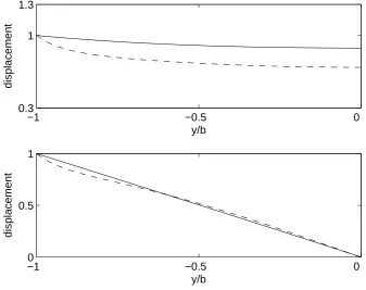
Figure 3.14 Flexural waves in a plate strip with free edges. Displacements across the plate strip at Ω =37.4 for (a) symmetric, (b) asymmetric motions: ― the S0, A0; – – the S1, A1; ···· the S2, A2 wave modes.

Figure 3.15 Flexural waves in a plate strip with free edges. Displacements in a half of the plate strip at ― Ω =0.7; – – Ω =37.4 for: (a) the S0, (b) A0 wave modes.

Figure 3.16 Flexural waves in a plate strip with free edges. Group velocities for

― symmetric; – – asymmetric wave modes.

Figure 3.17 Flexural waves in a plate strip with free edges. Dispersion curves for purely

imaginary and complex conjugate wavenumbers: (a) symmetric; (b) asymmetric wave modes; ○ numerical solutions to the dispersion equation.

Figure 3.18 Flexural waves in a plate strip with free edges. Loci of the wavenumbers for

positive going waves in the complex ξ -plane for the S_{i j,} mode: (a) i≥1,j≥2, j i= +1; (b) i≥0,j≥2, j i≥ +2 . Arrows indicate loci of

wavenumbers as frequency increases.

Figure 3.19 Flexural waves in a plate strip with free edges. Displacements along the plate width at various frequencies: (a) ― i, – – ii at Ω =3.59; (b) −·− (real part), ···· (imaginary part) for iii at Ω =4.71; (c) ― iv, – – v at Ω =6.28.

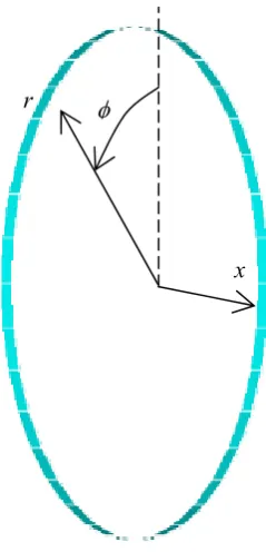
Figure 3.20 Coordinates of a ring.

Figure 3.21 Modelling of the ring using straight elements.

Figure 3.22 Waves in a ring. Dispersion curves for the modulus of (a) the real part, (b) the imaginary part: ― analytical solutions; ···· WFE results.

Figure 3.23 Waves in a ring. Relative errors in (a) the i=1; (b) the i=2 wavenumbers for

― a curved beam; – – a straight beam. Figure 3.24 Coordinates of a cylinder.

Figure 3.26 Dispersion curves for the predominantly flexural (i=1) waves in a cylinder, n=0,1,2,3,6,10,14: ― analytical solutions; – – WFE results.

Figure 3.27 Dispersion curves for the predominantly shear (i=2) and extensional (i=3) waves in a cylinder: ― analytical solutions; – – WFE results.

Figure 3.28 Dispersion curves for purely imaginary and complex wavenumbers of the i=1,2 (n=1,2,3,6) wave modes in a cylinder: ― analytical solutions; – – WFE results.

Figure 3.29 Dispersion curves for purely imaginary and complex wavenumbers of the i=3,4 (n=0,1,2) wave modes in a cylinder: ― analytical solutions; – – WFE results.

Figure 3.30 Group velocities associated with the i=1 (n=0,1,2,3,6,10,14) wave modes in a cylinder.

Figure 3.31 Group velocities associated with ― the i=2 (n=0,1,2); – – the i=3 (n=0) wave modes in a cylinder.

Figure 3.32 Power ratio for the i=1 wave modes in a cylinder calculated by analytical expressions: (a) n=0; (b) n=1; (c) n=2; (d) n=3. ― P P , – – _{f s} P P , _{ex s}

−·− P P . _{to s}

Figure 3.33 Power ratio associated with each variable for the i=1 wave modes in a cylinder using WFE results: (a) n=0; (b) n=1; (c) n=2; (d) n=3. −·− q , _x

― q , _r – – q_φ, −·−θ_x, ―θ_r, – –θ_φ. Figure 3.34 Section of a cylinder with finite length.

Figure 3.35 WFE model of a circumferential section of the cylinder using two series of the sections.

Figure 3.36 Dispersion curves for the propagating waves in a cylinder: ― analytical solutions; – – WFE results.

Figure 3.37 Power ratio associated with each variable for the i=1, n=1 wave mode in a cylinder: (a) between points A and B; (b) between points A and C. −·− q_φ,

– – q , _y ― q , _r −·−θ_φ, – –θ_y, ― θ_r.

Figure 3.38 Dispersion curves for purely imaginary and complex conjugates wavenumbers for the i=1, n=1-3; i=3, n=1; i=4, n=1 wave modes in a cylinder: ― analytical solutions; – – WFE results.

Figure 3.40 Dispersion curves for purely imaginary and complex conjugate wavenumbers for the i=2, n=2,4,6; i=3, n=2 (asymmetric) wave modes in a cylinder. Only WFE results are shown.

Figure 4.1 Procedure of forced response calculation using the wave approach. Figure 4.2 Waves directly excited by local harmonic excitation applied at a point. Figure 4.3 Wave reflection at a boundary.

Figure 4.4 Wave propagation in a waveguide. Figure 4.5 Wave amplitudes in a finite structure. Figure 4.6 Wave amplitudes in a ring.

Figure 4.7 The beam with sliding boundary conditions at both ends.

Figure 4.8 Magnitude of the input mobility of the beam: ― WFE result

(

)

···· analytical solution.

Figure 4.9 Magnitude of the input mobility of the beam: ― WFE result

(

)

···· analytical solution.

Figure 4.10 A thin plate with all edges simply-supported.

Figure 4.11 Magnitude of the input mobility of the plate: ― WFE result with

(

)

Re k_xΔ <_x 1, Im

(

)

Figure 4.12 Magnitude of the input mobility of the plate over wide frequency range:

― WFE result with Re

(

)

(

)

Figure 4.13 Magnitude of the input mobility of the plate: ― WFE result using all waves;

···· modal solution.

Figure 4.14 Magnitude of the input mobility of the plate: ― WFE result with

(

)

Re k_xΔ <_x 1, Im

(

)

Figure 4.15 Magnitude of the transfer mobility of the plate: ― WFE result with

(

)

Re k_xΔ <_x 1, Im

(

)

Figure 4.16 The forced response of the plate with η=0.01 at Ω =21.8. Figure 4.17 The forced response of the plate with η=0.03 at Ω =21.8. Figure 4.18 The forced response of the plate with η=0.1 at Ω =21.8. Figure 4.19 Cylinder with a finite length.

Figure 4.20 WFE models of the cylinder (a) in the ϕ-direction; (b) in the y-direction. Figure 4.21 (a) Magnitude and (b) phase of the input mobility of the cylinder: ― WFE

result with _Re

(

)

(

)

ϕ ϕ

Δ < Δ < ;···· modal solution.

Figure 4.22 (a) Magnitude and (b) phase of the input mobility of the cylinder: ― WFE result with _Re

(

)

(

)

ϕ ϕ

Figure 4.23 Magnitude of the input mobility of the cylinder: ― the WFE result using equation (4.2) with _Re

(

)

(

)

ϕ ϕ

Δ < Δ < ;···· modal solution. Figure 5.1 Cross-section of a tyre.

Figure 5.2 A tyre with an aluminium rim (195/65R15).

Figure 5.3 Segment of the WFE tyre model: (a) in the tyre cross-section; (b) in the circumferential direction.

Figure 5.4 Coordinates and a WFE model of the tyre section.

Figure 5.5 Dispersion curves of a straight segment for asymmetric modes: ― purely real; ···· purely imaginary; −·− complex conjugate wavenumbers. Ti denotes the shear wave mode. Small figure (a)-(d) illustrates the deformation associated with each wave mode. The solid line is the original shape and the dashed line is the deformed shape.

Figure 5.6 Dispersion curves of a straight segment for symmetric modes: ― purely real; ···· purely imaginary; −·− complex conjugate wavenumbers. Ti denotes the

shear wave mode. Small figure (a)-(c) illustrates the deformation associated with each wave mode. The solid line is the original shape and the dashed line is the deformed shape.

Figure 5.7 Dispersion curves of a curved segment for (a) the asymmetric, (b) symmetric modes: ― purely real; ···· purely imaginary; −·− complex conjugate wavenumbers. Ti denotes the shear wave mode.

Figure 5.8 Dispersion curves of a curved segment with internal pressure for (a) the asymmetric, (b) symmetric modes: ― purely real; ···· purely imaginary;

−·− complex conjugate wavenumbers. Ti denotes the shear wave mode.

Figure 5.9 Dispersion curves around the cut-on of the S2 mode: ― purely real; ···· purely imaginary; −·− complex conjugate wavenumbers.

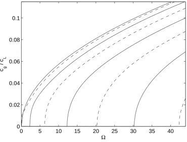
Figure 5.10 Dispersion curves for propagating waves of the symmetric modes. Figure 5.11 Group velocities for the S1, S2, Ts1 modes.

Figure 5.12 Group velocities for the S2, Ts1 modes.

Figure 5.13 Group velocities for the S2, Ts1 modes around the bifurcation. Figure 5.14 Group velocities for the damped S1, S2, Ts1 modes.

Figure 5.15 Experimental setup. Figure 5.16 Excitation arrangement.

Figure 5.18 Modelling of the excitation region: ― experimental; −− numerical modelling. Dots represent nodes where excitations applied. Dashed grid lines (····) represent FE.

Figure 5.19 (a) Magnitude and (b) phase of the input mobility at the tread centre of the tyre without internal pressure: ― the WFE result; ···· experiment.

Figure 5.20 (a) Magnitude and (b) phase of the input mobility at the tread centre of the tyre with internal pressure: ― the WFE result; ···· experiment.

Figure 5.21 (a) Magnitude and (b) phase of the predicted input mobility of the tyre for

― the finite area excitation; −− a point excitation.

Figure 5.22 (a) Magnitude and (b) phase of the predicted input mobility of the tyre for

― the uniform force excitation; ···· uniform velocity excitation.

Figure 5.23 (a) Magnitude and (b) phase of the predicted input mobility of the tyre in

― the radial direction; −− the circumferential direction. Figure A2.1 Muller’s method using a quadratic function.

Figure A2.2 Example of a contour plot for f z .

( )

Figure A2.3 Contour plot of (a) Re

{

( )

}

{

( )

}

Figure A3.1 Cross-section of the tyre. Right hand side exaggerates the structure for clarity. Figure A3.2 Laminate of two FRR sheets with angle of ±θ .

Figure A3.3 Modelling of internal pressure using surface loads: (a) regions where the loads applied (masked regions); (b) pressure distribution in the tread region. Figure A3.4 Relationship between the Young’s modulus and the reduced frequency. Figure A3.5 Relationship between the loss factor and the reduced frequency.

Figure A3.6 Relationship between temperature and the shift factor.

Figure A3.7 FE model of a tyre using (a) 28 FEs; (b) 50 FEs in the cross-section.

Figure A3.8 (a) Magnitude and (b) phase of the predicted input mobilities of the tyre using

― 28 elements; −− 50 elements in the cross-section.

Table 5.1 Summary of equipment.

Table A3.1 Material properties of rubber in SI units. Significant figures are rounded to 1 as they are commercially sensitive.

Chapter 1: Introduction

Chapter 1

INTRODUCTION

1.1 Introduction

Analysis of wave propagation in a medium is of great concern for acoustical, electrical, electromagnetical and structural engineers. Examples include sound propagation in air, the transmission of radio waves, the transmission of seismic tremors in the earth and structure-borne sound. In particular, analysis of waves in structural waveguides is of concern in this thesis. Many structures are uniform in direction and can hence be regarded as one-dimensional waveguides along which mechanical disturbances propagate. Examples of such waveguides include a rod, a beam, a plate, a cylinder, a railway track and a tyre. Throughout this thesis, waveguides are assumed to be uniform such that the material properties and the cross-section geometry are invariant along the axis of the waveguide.

Chapter 1: Introduction

noted that analytical solutions involve assumptions and the model might become complicated in various circumstances, especially when the construction of the structure becomes complicated or at high frequencies.

For two-dimensional waveguides analytical solutions are available only for specific cases such as an isotropic thin plate with simply-supported boundary conditions in which the displacement can be decomposed into harmonic components, e.g. [1]. Analytical dispersion equations may be transcendental for general waveguides such as a plate strip with free edges. Solutions to the transcendental analytical equation need to be found numerically and the exact solutions cannot be obtained. The similar discussion holds for other analytical methods such as the dynamic stiffness method [5] or the transfer matrix method [6].

In summary, therefore, the analytical solutions may involve approximations of unknown validity and they may be difficult or impossible to obtain for general waveguides with arbitrary complicated cross-sections and boundary conditions. Examples include a railway track and a tyre for both of which the geometry is complicated. To investigate the dynamics of general waveguides numerical methods have been proposed, such as the spectral finite element method [7] and the wave finite element (WFE) method [8,9].

The present work concerns the WFE method. A small section of the waveguide is modelled using finite element analysis (FEA). This yields the mass, damping and stiffness matrices, which are subsequently post-processed in conjunction with a periodicity condition to form the eigenvalue problem. The eigenvalues and eigenvectors represent the free wave propagation characteristics. Since the existing element libraries and commercial finite element (FE) packages can be utilised to model complicated structures, the WFE method is a powerful tool to investigate the dynamics of such structures.

The objectives of the present work are to extend the WFE method for the prediction of vibrational behaviour of structures in terms of wave motion. In particular it concerns the applications to one-dimensional waveguide structures with arbitrary complexities in the cross-section or complicated dispersion characteristics. The particular contributions concern numerical issues, the forced response and various applications including the forced response of an automotive tyre.

Chapter 1: Introduction

method can be applied to any one-dimensional waveguides with arbitrary complexities in their cross-sections. Applications to a plate strip and an automotive tyre are presented. In the latter, frequency dependent material properties are involved and predictions are compared with experiment.

In the remainder of this chapter existing methods are reviewed and the WFE method is described in detail. The contents and original contributions of this thesis are then described.

1.2 Review of Analysis Methods for Dynamics of Waveguides

In this section analysis methods for the dynamics of waveguides are reviewed. In subsection 1.2.1 the classical analytical approach is first described. The analytical solutions are found from the analytical equation of motion. The general wave approach is also reviewed to give wave motion in general waveguides. Other analytical methods such as the dynamic stiffness method and the transfer matrix method are reviewed in subsection 1.2.2. However, such analytical approaches are in general applicable only to simple waveguides. Numerical methods such as the spectral finite element method and the WFE method are then needed to investigate waves in general waveguides. These numerical methods are described in subsection 1.2.3.

1.2.1 Analytical Method (Wave Approach)

In this subsection the classical analytical method for determining wave motion in structural waveguides is reviewed. Analytical determinations for free wave propagation, reflection and transmission, and forced response are described. The general wave approach is reviewed in which wave propagation, reflection and transmission are considered.

Free Wave Propagation

Chapter 1: Introduction

4 2

4 2 0

w w

C

x t

∂ ₊ ∂ ₌

∂ ∂ (1.1)

where w is the translational displacement, x is the direction along the axis of the beam, t is time and C is the constant given from its material properties and geometry of the cross-section. Assuming time- and space-harmonic motion, the displacement is written as

jkx j t

w ae= − eω (1.2)

where k is the wavenumber, ω is the angular frequency, a is a wave amplitude and 1

j= − . Substituting the displacement (1.2) into the governing equation gives the analytical dispersion equation of the beam as

4 2

k =Cω . (1.3)

The beam holds four freely propagating waves with their wavenumbers being 4 2

k = ± Cω , 2

4 j Cω

± . The first two wavenumbers describe propagating waves and the latter two are nearfield waves. The positive real and negative imaginary wavenumbers are associated with the positive-going waves so that the waves propagate in the positive direction of the beam and the other wavenumbers are associated with the negative-going waves. Once the dispersion equation, e.g. equation (1.3), is obtained, the phase velocity ω k and the group velocity ∂ ∂ω k can be calculated. The same approach can be used to waveguides where the analytical equations of motion are available.

Reflection and Transmission

When waves propagate along a waveguide, the waves might impinge on such as a boundary, a discontinuity and so on. The incident waves will reflect at boundaries and may reflect and transmit at discontinuities, e.g. [1,2,11].

Chapter 1: Introduction

(

)

i rP rN

w= a e− +a e +a e eω (1.4)

where a_i, a_rP, a_rN are the amplitudes of the incident, reflected propagating and reflected nearfield waves, respectively. Depending on the boundary condition, a combination of displacements and forces is given at the boundary such that the reflection coefficients,

rP i

a a and a_rN a_i , can be calculated. For a free boundary condition for the beam, for example, the reflection coefficients are given by a_rP a_i = −j and a_rN a_i = −1 j [1]. The complex values of the coefficient indicate that phase shifts occur in the reflected waves relative to the incident wave. In this case both propagating and nearfield waves are generated for one incident propagating wave such that wave mode conversion occurs. Knowledge of the phase change at boundaries enables one to determine the natural frequencies of a finite waveguide. When the total phase change of the propagating wave along the waveguide satisfies certain condition, system motion intensifies. Such an approach is termed as the phase closure principle [3] or phase coincidence [12].

When a wave impinges on a discontinuity such as a point mass, both reflected and transmitted waves may be generated. The continuity of displacement at the discontinuity and force equilibrium at the discontinuity give the reflection coefficients and transmission coefficients [1,2,11]. For the beam the propagating and nearfield waves may be generated for both the reflected and transmitted waves such that four waves in total can be generated. The reflection and transmission coefficients are frequency dependent in general.

Forced Response

Chapter 1: Introduction

General Wave Approach

The approach described above can be applied to other cases where the equation of motion can be analytically expressed. The examples include the Timoshenko beam, a beam subjected to in-plane tension and on an elastic foundation, a general rod, a ring and plates, e.g. [1]. For waveguides in which there are many wave modes, wave motion is conveniently expressed in matrix form. Formulation for the dynamic behaviour of waveguides using the wave approach is well-conditioned. This is important for general waveguides for which numerical issues are likely to occur.

Several works about the general wave approach are reviewed here. Mace [14] studied the vibrational behaviour of a beam based on propagation, reflection and transmission of waves including the flexural nearfield waves. Inclusion of nearfield waves is particularly important when the local behaviour around a discontinuity or an excitation is of concern and when two nearfield waves propagate in opposite directions, since they can carry power [15,16]. The amplitudes of the waves and the excitation are expressed in vector forms and wave propagation, reflection and transmission are described in matrix forms. Consequences of reciprocity were shown for the reflection coefficient matrix [17] and the transmission coefficient matrix [18] including nearfield waves.

Many applications of the wave approach can be found in the literature. Miller and Von Flotow [15] used the wave approach to investigate the power in an assemblage of one-dimensional members. The coupling power between two end-coupled beams was presented by Mace [19] and that between two plates was shown by Wester and Mace [20]. Lee et al [21] analysed the power reflection and transmission for two beams connected with a U-shape beam. Yong and Lin [22] used the wave approach to calculate the forced response of a periodically supported beam. Harland et al [23] demonstrated the systematic implementation of the wave approach for arbitrary waveguides and considered in detail the cases of a sandwich beam, jointed beams and a beam with a local discontinuity.

Chapter 1: Introduction

1.2.2 Other Analytical Methods

To investigate the dynamics of waveguides some other methods have been proposed, e.g. [24]. In this subsection some of these other analytical methods are reviewed. They include the dynamic stiffness method, the transfer matrix method, the receptance method and the spectral element method.

Dynamic Stiffness Method:

The dynamic stiffness method [5] is sometimes termed the dynamic stiffness matrix method [25] or the dynamic element method [26]. A section of a structure is modelled by the analytical relationships between displacements and forces applied at the ends or edges of the section. The equation of motion for time-harmonic behaviour is expressed as

LL LR L L RL RR R R

⎡ ⎤ ⎡ ⎤ ⎡ ⎤

=

⎢ ⎥ ⎢ ⎥ ⎢ ⎥

⎣ ⎦ ⎣ ⎦ ⎣ ⎦

D D q f

D D q f (1.5)

where D is the dynamic stiffness matrix, the subscripts L and R represent the left and right hands of the section, q and f are the displacement and force vectors respectively. The matrix D is given in the frequency domain and its elements are frequency dependent.

Some applications can be seen in literature. Langley [27] analysed power in a beam and a truss structure. Lee and Thompson [28] applied the method to helical springs. A series of works by Banerjee present the dynamic stiffness matrix for various one-dimensional waveguides, e.g. [29,30]. Langley [31,32] applied the method to investigate free and forced vibrations of the two-dimensional structures but only for simply-supported edges where the displacement along one-dimension can be decomposed into harmonic components.

The dynamic stiffness matrix can be expanded into a power series in terms of ω [26] such that

( )

( )

0

i i i

ω ∞ ω

=

=

∑

Chapter 1: Introduction

The resulting matrices

( )

D can be regarded as the consistent stiffness matrix (i=0), the consistent mass matrix (i=1) and higher order correction terms

(

)

Transfer Matrix Method:

The transfer matrix method [6], or Holzer’s method [33], describes the change of wave modes, or the state vector, at two different locations (cross-sections) along the waveguide. The equation of motion of the waveguide are in general expressed as

11 12 21 22

L R

L R

⎡ ⎤ ⎡ ⎤ ⎡ ⎤

=

⎢ ⎥ ⎢ ⎥ ⎢ ⎥

⎣ ⎦ ⎣ ⎦ ⎣ ⎦

T T q q

T T f f . (1.7)

The analytical derivation of the transfer matrix T is summarised in [6]. Extensive examples for series of spring/mass and one-dimensional waveguides can be found in [6].

Applications to one-dimensional periodic structures and continuous waveguides joined together were studied by Lin and Donaldson [34]. The response to a point force is also considered in [34]. Lin and Yang considered free vibration of a disordered periodic beam [35]. It should be noted that the transfer matrix method can suffer from numerical ill-conditioning when solutions are to be found numerically [24,34].

Receptance Method:

Mead et al developed the receptance method mainly to analyse waves in periodic structures, e.g. [3,36]. The method starts from the equation of motion using the receptance matrix, i.e. reciprocal of the dynamic stiffness matrix, formed in the same manner as equation (1.5). A periodicity condition [37]

,

R L

R L λ λ

= =

q q

f f (1.8)

is then applied to the equation motion to give the polynomial eigenvalue problem in the form, e.g. [3],

( )

(

( )

( )

)

( )

2

λ ω λ ω ω ω

Chapter 1: Introduction

where α is the receptance matrix. The values of λ may be calculated for each given ω and indicate how waves propagate or decay at a particular frequency.

An application to a beam with periodic supports can be seen in [36] and also [38] where effects of the damping are considered. Waves in periodic structures are considered for mono-coupled systems in [39] and for multi-mono-coupled systems in [40] where the complex conjugate wavenumbers are described. Effects of a point discontinuity on waves in periodic structures were considered in [41] and the response to convected loadings was reported in [42]. Coupling of the in-plane and flexural waves in a layered beam is described in [43]. The receptance matrix may be formed using FEA [44,45] but details are omitted here.

Spectral Element Method:

The spectral element method starts from writing the displacement along the uniform (x-) direction in the form of equation (1.2). Substituting the displacements (1.2) into the analytical governing equations gives the relationships between displacements and forces at a location. The spectral element for a segment of the waveguide between two nodes then follows. The spectral element can also be defined for a section of a waveguide extending to infinity. Such a semi-infinite spectral element is termed as a single-noded or throw-off element in [11]. Doyle [11] summarised the method and showed applications to simple waveguides.

1.2.3 Numerical Methods

Various analytical methods have been reviewed in subsections 1.2.1 and 1.2.2. The methods, however, require that the equation of motion of the waveguide is known and can be solved analytically. General complicated waveguides are not amenable to analytical solutions such that numerical methods have been then proposed, e.g. the spectral finite element method and the WFE method. These numerical methods are reviewed in this subsection.

Finite Element Method (FEM):

Chapter 1: Introduction

functions are defined to describe the motion of the system. These are in general low-order polynomials, e.g. [46,47]. Higher order shape functions such as p-elements, e.g. [47], may be defined. The system motion is then described in the time domain in terms of a discrete number of nodal degrees of freedom (DOFs) such that

( )

+ + =

Kq Cq Mq f& && (1.10)

where K, C, M are the stiffness, damping and mass matrices and q_& is the derivative of q with respect to time. Since the size of elements should be small enough, e.g. [46], the size of the FE model, and hence the calculation cost, is larger at higher frequencies.

Spectral Finite Element method:

To analyse wave motion in general waveguides, the most common approach is perhaps the spectral finite element method, e.g. [11,48], or sometimes termed the waveguide finite element method [7]. Displacements are separately expressed in the direction of wave propagation, x, and over the cross-section, (y, z) such that [7,11,48]

(

)

( )

w x y z t ₌aϑ y z e− eω _(1.11)

where ϑ

( )

(

)

i i

jk ω

⎡ _{− −} ⎤ ₌

⎢ ⎥

⎣

∑

where K and M are the spectral matrices and i is an integer. The solutions may be found for given k to give real ω for the standard eigenvalue problem. Alternatively, solutions of

k might be found for given real ω solving the polynomial eigenvalue problem.

Chapter 1: Introduction

off frequencies. Finnveden [48] also applied the method to analyse wave motion in a thin wall structure and the results were used as input parameters to a statistical energy analysis model [50]. The spectral finite element method was also applied to laminated composite plates by Datta et al [51] and viscoelastic laminates by Shorter [52]. Extensive works were reported by Nilsson [7] where the spectral finite element method is applied to a thin wall structures, a fluid-filled pipe and a tyre.

However, a drawback of the spectral finite element method is the fact that the method needs appropriate spectral elements to be derived on demand for general waveguides, which is not an insignificant task.

Wave Finite Element (WFE) Method:

The WFE method is an alternative to investigate wave motion in general complicated waveguides. The method starts from modelling a short section of a waveguide using conventional FEs such that the equation of motion is given in terms of a discrete finite number of DOFs, as in equation (1.10). For time-harmonic motion equation (1.10) gives the same form as the dynamic stiffness method, i.e. equation (1.5). The transfer matrix (1.7) can be formed using elements of the dynamic stiffness matrix and applying a periodicity condition (1.8) to the equation (1.7) gives the eigenvalue problem.

The eigenvalues and eigenvectors represent the free wave propagation characteristics such as the wavenumbers and wave modes. This thesis concerns the WFE method and the method is specifically reviewed in detail in the next section.

1.3 Wave Finite Element Method

Chapter 1: Introduction

efficiency is described in [53] where the method is termed the scale independent element method.

1.3.1 Analysis of Waves using Finite Elements for Periodic Structures

The WFE method grew out of research concerning FEA of periodic structures done by Orris and Petyt [44,45]. They used the finite elements to model periodic structures and applied the receptance method proposed by Mead, e.g. [3,36]. Extensive work has been done by Abdel-Rahmen [54]. Free wave propagation in one-, two- and three-dimensions was analysed for periodic structures using an FE model of a single periodic section. A periodicity condition was applied to the equation of motion formed from the FE model and the eigenvalue problem was formulated. Free wave propagation characteristics were determined from solutions to the eigenvalue problem. Forced responses to convected random pressure field excitation were considered.

The similar approach was applied to predict free wave propagation in truss beam structures by Signorelli and Von Flotow [55] where the complex wave modes are described. Accorsi and Bennett [56] analysed free wave propagation in a stiffened cylinder and Bennett and Accorsi investigated effects of the curvature along the axis of the cylinder [57].

1.3.2 Free Wave Propagation

Perhaps the first application to continuous structures was the work of Thompson [58] concerning railway tracks. For simple waveguides, Mace et al [8] showed free wave propagation in a rod, a beam and a plate strip with simply-supported edges using the WFE method. They also presented the free wave propagation in a layered sandwich beam.

Chapter 1: Introduction

the WFE method [62]. Free wave propagation in a fluid-filled pipe was also presented by Maess et al [63]. They formulated an eigenvalue problem using elements of the transfer matrix and numerical solutions were found with initial estimates. The WFE method was extended to analyse free wave propagation in two-dimensional waveguides by Manconi and Mace [64,65].

1.3.3 Forced Response

Forced response is of interest when an excitation is applied to a waveguide. Only a few papers describe the forced response using the WFE method. Duhamel et al [9] presented the formulation for calculating the forced response using a recurrence relationship. Thompson [58] calculated the forced response based on the receptance approach for the railway track. A similar, but different approach was used to analyse the forced response of a railway track by Gry [60]. However, all the approaches have ill-conditioning problems for general waveguides in which there are many wave modes.

1.3.4 Numerical Issues

In predictions using the WFE method various numerical issues occur. However, only a few papers describe such numerical issues. Several papers describe the ill-conditioning of the eigenvalue problem using the transfer matrix and reformulate the eigenvalue problem in a different form. A novel formulation for improving the conditioning of the eigenvalue problem was proposed using the symplectic relationship of the transfer matrix by Zhong and Williams [66]. Several papers used the method, called Zhong’s method in this thesis, to improve the conditioning [8,60,62,67,68].

Since the WFE method starts from the FE model of a section of a waveguide, FE discretisation errors occur. Duhamel et al [67] and Mace et al [8] demonstrated FE discretisation errors occurring in the WFE method. The aliasing effect due to the discretisation and the spatial periodicity was reported by Ichchou et al [10].

However, such numerical issues have not been reported in detail. In this thesis, numerical issues are discussed in detail and methods are proposed to reduce numerical errors.

Chapter 1: Introduction

1.4 Outline of the Thesis

The thesis is outlined in this section. This thesis concerns formulation of the WFE method and its application to free wave propagation and the forced response of waveguides of arbitrary complexity in their cross-sections. Causes of numerical errors in the predicted results using the WFE method are investigated and methods for reducing errors are proposed. Applications of the WFE method to complicated structures are then presented. The forced response is calculated using the wave approach with well-conditioned formulations and numerical examples are shown. Free and forced vibrations of a tyre are then predicted and the predicted forced response is compared with experiment. Throughout this thesis, ANSYS 7.1 [69] is used to model sections of waveguides. All the subsequent calculations were performed using MATLABTM _7.0.4.

In chapter 1 the introduction is given and relevant literature is reviewed. The thesis is outlined and contributions of this thesis are then described.

In chapter 2, formulations of the WFE method are introduced. Numerical errors occurring in the WFE results are discussed. FE discretisation error and error due to round-off of inertia terms are described with particular reference to the example of an Euler-Bernoulli beam. A method of concatenating elements is proposed to reduce the round-off of inertia terms. Approximate expressions for the dynamic condensation of DOFs associated with internal nodes are derived to reduce calculation cost. Errors occurring in numerically solving the eigenvalue problem are also described. Zhong’s method is used for improving the conditioning of the eigenvalue problem. An application of singular value decomposition (SVD) is proposed to reduce errors in numerically determining eigenvectors. An illustrative example of free wave propagation in a plate strip with simply-supported edges is shown considering numerical issues. Effects of how the cross-section is modelled are investigated. Methods of predicting the group velocity are described and use of the power and energy relationship is shown to be reliable.

Chapter 1: Introduction

Complicated wave behaviour is seen. Curve veering between two different purely real or two different imaginary wavenumbers is observed. Non-zero cut-on phenomena are observed where complex conjugate wavenumbers become purely real non-zero wavenumbers. Waves for which the directions of the phase and group velocities are of opposite signs are seen. Bifurcations from complex conjugate to two different purely imaginary wavenumbers or two imaginary to complex conjugate wavenumbers are observed. Decomposition of power is used to investigate characteristics of each wave mode in a cylindrical strip.

In chapter 4, formulations of forced response calculation are described. A well-conditioned formulation for numerically determining the amplitudes of directly excited waves is proposed using the orthogonality relationship between the left and right eigenvectors. Wave amplitudes are calculated considering wave propagation and subsequent reflection at boundaries. The response is then determined by superimposing the wave amplitudes at the response point. The formulations to determine responses are explicitly described. Forced responses of a beam, a plate and a cylinder are shown. Inclusion of rapidly decaying nearfield waves is discussed.

In chapter 5, the WFE method is used to predict free and forced vibrations of a tyre as an example of a practical application. Frequency dependent material properties of rubber are included. Free wave propagation is shown including attenuating waves for the tyre with and without internal pressure. Results of the forced response are compared with experiment. Effects of the size of the region of excitation are described. This strongly affects the power injected into wave modes, especially at high frequencies, and contribution of the finite shear stiffness to the response.

In chapter 6, some conclusions are drawn. Possible further work is suggested.

1.5 Contributions of this Thesis

The original contributions of this thesis are as follows.

Chapter 1: Introduction

terms. Approximate expressions for dynamic condensation of DOFs associated with internal nodes are derived [70].

• Numerical issues remain even when Zhong’s method is used to reformulate the eigenvalue problem. An application of SVD is proposed to reduce errors in numerically determining eigenvectors [70,71].

• Three methods for predicting the group velocity are described and relative errors in the group velocity compared. Use of the power and energy relationship is then shown to be reliable [70,71].

• Freely propagating flexural waves are predicted including attenuating waves and results are compared with numerical solutions to the analytical dispersion equation. Bifurcations from the complex conjugate to purely imaginary wavenumbers and from purely imaginary to complex conjugate wavenumbers are observed [72].

• Decomposition of the power is proposed. The approach can be used for determining the DOFs to be condensed or to be removed. Such manipulation can improve the conditioning due to the smaller size of matrices. The approach is also applied to investigate wave characteristics of each wave mode.

• The wave approach is applied to calculate forced response. A well-conditioned formulation for determining the amplitudes of directly excited waves is proposed using the orthogonality relationship between the left and right eigenvectors [73,74].

Chapter 2: Free Wave Propagation

Chapter 2

FREE WAVE PROPAGATION

2.1 Introduction

Many waveguides are uniform in one-direction while their cross-sections may have a complicated construction. The dynamic properties of such waveguides can be expressed in terms of wave properties such as the wavenumbers and wave modes. In this chapter, the theory and formulations of the WFE method are introduced to predict their wave properties. Only a short section of a waveguide is modelled using a conventional FEA. A complicated cross-section can be straightforwardly modelled using existing FE libraries and FE commercial packages. The dynamic stiffness matrix of a short section of a waveguide is obtained and the matrix rearranged and partitioned to form the transfer matrix. The free wave propagation characteristic may be obtained from the transfer matrix by applying a periodicity condition [37].

In this chapter, various numerical issues involved in obtaining accurate results using the WFE method are discussed. Causes of numerical errors are investigated and implementations of the WFE method to reduce these errors are proposed. The discussions include a method using concatenating elements and conditioning of the eigenvalue problem to reduce numerical errors. The group velocity is numerically estimated in three ways and the accuracy is investigated. Some outcomes shown in this chapter have been presented in [70,71].

2.2 Transfer Matrix

Chapter 2: Free Wave Propagation

eigenvectors of the eigenvalue problem represent phase or magnitude changes of waves over the section and associated wave modes respectively.

2.2.1 Dynamic Stiffness Matrix of a Section of a Waveguide

Consider a short of section of length Δ of a uniform waveguide as shown in Figure 2.1. The equation of motion of the section can be written as

=

Dq f (2.1)

where

2

jω ω

= + −

D K C M (2.2)

is the dynamic stiffness matrix, q is the nodal displacement vector, f is the vector of nodal forces, K , C , M are the stiffness, damping and mass matrices (termed the element matrices), which may be formed using a commercial FE package, j= −1 and ω is angular frequency. Time harmonic motion _ej tω _{is implicit throughout this thesis and suppressed for} brevity. Equation (2.1) can be expressed in matrix form as

LL LR L L RL RR R R

⎡ ⎤ ⎡ ⎤ ⎡ ⎤

=

⎢ ⎥ ⎢ ⎥ ⎢ ⎥

⎣ ⎦ ⎣ ⎦ ⎣ ⎦

D D q f

D D q f (2.3)

where the subscripts L and R represent the left and right hand side of the section. The WFE method starts from equation (2.3) and the eigenvalue problem is formulated using the elements of equation (2.3). For uniform waveguides, the following relationships hold:

T _, T _, T

LL = LL RR = RR LR = RL

D D D D D D (2.4)

and

,

RRij LLij RLij LRij

D = ±D D = ±D (2.5)

where _⋅T _{indicates the transpose and the signs in equations (2.5) depend on whether the} degrees of freedom (DOFs) at the element interface are symmetric or anti-symmetric for the

Chapter 2: Free Wave Propagation

If the section has internal nodes as shown in Figure 2.2, the associated DOFs can be condensed. When no external force is applied to the internal nodes the equation of motion may be expressed as

E E EE EI I IE II ⎡ ⎤ ⎡ ⎤ ⎡ ⎤₌ ⎢ ⎥ ⎢ ⎥ ⎢ ⎥ ⎣ ⎦ ⎣ ⎦ ⎣ ⎦ q f D D q 0 D D % %

% % (2.6)

where

, , , L , L

LL LR LI

EE EI IE IL IR E E

R R

RL RR RI

⎡ ⎤ ⎡ ⎤ _{⎡ ⎤} ⎡ ⎤ ⎡ ⎤

=_{⎢ ⎥} =_{⎢ ⎥} =_{⎣ ⎦} =_{⎢ ⎥} =_{⎢ ⎥}

⎣ ⎦ ⎣ ⎦

⎣ ⎦ ⎣ ⎦

q f

D D D

D D D D D q f

q f

D D D

% % %

% % % % %

% % % (2.7)

and the superscript ~⋅ denotes that the section has internal nodes and is not condensed. The subscript E or I represents that DOFs are associated with edge nodes or internal nodes of the section. The DOFs associated with the internal nodes can be condensed as [75]

T

E = E

R DRq% % % f (2.8)

where 1 II IE − ⎡ ⎤ = ⎢₋ ⎥ ⎣ ⎦ I R D D %

% % (2.9)

and I is the identity matrix. The matrix R% transforms the original basis into the condensed basis. Expanding equation (2.8) gives

1

EE EI II IE E E

−

⎡ − ⎤ =

⎣D% D D D% % % ⎦q f . (2.10)

Equation (2.8) can similarly be used to condense the element matrices by expanding 2

ω

= −

D K% % M% [75]. It should be noted that the dynamically condensed element matrices become frequency dependent.