Changing Circumstances and Leveled Commitment:
A Compensatory Approach to Contracting
Ilja Ponka and Nicholas R. Jennings
University of Southampton
School of Electronics and Computer Science
Southampton SO17 1BJ, United Kingdom
{
imp04r, nrj
}
@ecs.soton.ac.uk
Abstract
In dynamic and uncertain e-commerce settings, the value of contracts can change after they have been entered into. Sometimes this can make the contract in question counter-productive to the affected parties. Given this, leveled com-mitment contracts, in which one agent pays the other a fee to be released from their decommitment, are widely used. However, these fees are often seen only as a deterrent of de-commitment and the fact that the dede-commitment also affects the other party and the society in general is usually ignored. This paper investigates an alternative view, coming from law, that sees the decommitment fees as a means of compensat-ing the victim for their loss. Moreover, we show that these compensatory policies can outperform their traditional non-compensatory counterparts in terms of total utility (the sum of all agent’s utilities) in situations in which the utility of one of the parties decreases after the contract has been entered into, but before it is due to be performed.
1
Introduction
In fast-moving electronic markets, hundreds of contracts can be formed in a matter of seconds. However, in dynamic, ever-changing environments, sometimes the parties of these contracts may live to regret their choices. A better alternative may surface only seconds after agreeing to something or the circumstances may change and turn a contract from lucrative into disastrous. On the other hand, contracts (or commit-ments about performing a service at a later time) have been seen as an essential requirement for any type of predictable behaviour in such systems [5]. Against this background, an often used compromise is Sandholm and Lesser’s [7]leveled commitment contract, which:
• allows unilateral decommitting for both parties at any time, but
• requires the decommitting party to pay the opponent a monetary fee (called a decommitting fee) for doing so. This allows a party to abandon a contract that has become counter-productive to it; that is, its utility has become
nega-tive. Now, because the party must pay the penalty in order to decommit, a decommitment occurs only if the decommit-ment improves the decommitter’s utility more than the fee to be paid reduces it. In the literature, the decommitment fee is therefore mostly seen as a deterrent of decommitment. This view, however, overlooks the effect a decommitment has on the other party (the victim) and on the society in general. In particular, the decommitment will usually decrease the utility of the victim, because he will lose the profit he was expecting and it is also possible that he has accrued some costs (preparing for its performance) before decommitment occurs. When the contract is abandoned, these costs may have been wasted. Now, if these lost profits and accrued costs outweigh the benefit the decommitter receives from de-commitment, the decommitment actually decreases the sum of utilities of parties and is therefore detrimental to the wel-fare of the society as a whole.
In contrast, the law has traditionally taken another view, that of the victim’s. In cases of non-performance, the vic-tim (in most legal systems) is entitled to damages (there may be other remedies in some situations and in some legal sys-tems, but we concentrate on damages here) and the aim of damages is usually to put the victim financially in the same position as if the contract had been performed appropriately [8]. That is, the damages compensate the victim for the loss that the non-performance causes. The economic efficiency of this rule has been investigated in the law and economics literature in the area of efficient breach theory [2]. The con-clusion of this work is that this is the optimal policy from the society’s point of view. In particular, by setting the dam-ages (decommitment fee) equal to the damage caused by the decommitment to the other party, a breach (decommitment) occurs when and only when the benefit to the decommitter is greater than the damage to the victim. Therefore decom-mitment always increases the total welfare of the society.
decommit-ment causes to the opponent. Any policy that does not have this goal, is callednon-compensatory.1 Most of the poli-cies used in the literature so far are non-compensatory, al-though many papers (e.g. [1] and [6]) have suggested using fees that increase over time. Although the reason for this is usually not explicitly stated, this type of fee can be seen as being both more compensatory and more fair than the con-stant fee. Also some partially compensatory policies have been suggested (e.g. [3]), but no consistent theory for do-ing so has been presented. We will address these shortings by using ideas from contract law to create novel com-pensatory decommitment policies and show how they (under certain circumstances) can be used to improve total utility in e-commerce settings.
However, the compensatory approach has its problems. For example, Andersson and Sandholm [1] have argued that if the victim’s actual loss is not known, he has an incentive to overstate it in order to keep the contract or to make additional profit. In law, this problem is avoided by making the victim show the actual amount of loss in a court of law after the final outcome and losses are known exactly. This incurs consider-able costs to the parties and is often slow. In global electronic markets of relatively low-value services, both characteristics are undesirable. We therefore suggest using the opponent’s expected or average losses as a decommitment fee. These expected losses are estimated and given to all parties by the neutral marketplace. In many markets, this type of informa-tion is available or can be obtained at reasonable costs.2 In
addition, we will show that even relatively inaccurate esti-mates can improve the total utility over non-compensatory alternatives.
We will also show that the better the estimates are, the more they will lead to better total utilities. Since in the long run, the marketplaces that generate most welfare to their partic-ipants are likely to be the most popular, the neutral market-place has an incentive to improve its estimates. Compen-sating for these losses also has a fairness aspect that many humans find appealing. In dynamic environments, all par-ties are occationally decommitters and sometimes victims, so the markets that treat both cases fairly may find greater acceptance among the (potential) users.
The rest of the paper is structured as follows. Section 2 introduces our model of electronic markets, in which the parties make contracts. Section 3 discusses the various de-commitment policies. Section 4 details our experiments and findings. Finally, section 5 concludes.
1The distinction is not always clear-cut, because some non-compensatory policies can be non-compensatory in some circumstances. The important requirement for the compensatory policies is that theyalwaystry to compensate for the victim’s loss.
2For example, in many industries the product, its preparation process and costs are well-known (e.g. printing a book). Also if all providers use similar technologies or sub-providers (e.g. teleoperators renting capacity from the same network company), it may be possible to estimate the costs.
2
The Marketplace Model
We consider a market of buyers and sellers for one service. We refer with subscriptbto a single buyer (consumer) and with subscriptsto a single seller (provider) in this market. We are especially interested in their utility,Ub andUs re-spectively. The timetis discrete and divided into turns.
We assume that all participants expect the delivery of the service to occur at the same timetdelivery(there are separate markets for different delivery times and other services). In the beginning (t0= 0) there aren0buyers andn0sellers in the market. This is to ensure that negotiations can start from the beginning. Over time, some buyers and sellers enter and some may exit. The numbers of entries for the parties are independent variables, but follow the same standard Poisson distribution, with the parameterλ(t) = itdelivery−t
tdelivery , where
iis the basic entry intensity andtis the current turn. This formulation means that entries are more probable earlier in the experiment. This is because we assume that the provision of the service takes time,tp, and this time is different from one provider to another (selected at random). The nearer the time of performance, the fewer providers are likely to be able provide the service in time. In the experiments we discuss in this paper, we havetdelivery= 1000,n0= 50andib= 0.4, which gives us an expected population size of250during an individual experimental run.
On the other hand, we assume that the provision costs money. Specifically, in order to provide the product at the delivery time, the providershas to invest cost cs at time
tc,s(< tdelivery). Each provider has a qualityqs, which is selected at random fromUniform(0,1). The cost is a func-tion of quality and time:
Cs(qs, t) =
0, ift < tc,s, 0.5qs, ift≥tc,s.
Here, we have six different settings fortc,s: • any:Uniform(te,s+ 1,999),
• second half:Uniform(max(500, te,s+ 1),999),
• last quarter:Uniform(max(750, te,s+ 1),999),
• last 100:Uniform(max(900, te,s+ 1),999),
• turns 925-975:Uniform(max(925, te,s+ 1),975),
• turn 950:950,
service, it will exit the market. The provider’s utility for a contract is:Us(p, cs) =p−cs, wherepis the contract price. The consumers do not have costs, but each consumer
b has a deadline tx,b, which is selected at random from
Uniform(te,b + 1, tdelivery), where te,b is the time con-sumerb entered the market. The consumer’s utility for the contract isUb(q, p) = Vb(q)−p, where the value function
Vb(q)is:
Vb(q) =
0, ifq < qbmin,
v(q), ifqbmin≤q≤qbmax,
v(qmax
b ), ifq > qbmax,
wherev(q)is the consumers’ common value function,qbmin andqbmaxare consumer specific parameters of that function. Here we assume simply thatv(q) =q. This means that each consumer has a minimum useful qualityqbminand any ser-vice that does not offer at least this, is worthless (Vb = 0). On the other hand, the consumer also has a maximum use-ful quality,qbmax, which gives him his full utility. Any im-provement above this level does not increase the value of the service to the consumer in question. The parametersqbmin andqmaxb are selected for each consumer independently at random fromUniform(0,0.5)andUniform(0.5,1.0) re-spectively. The consumer’s reservation price for a given ser-vice is then equal to its value.
The buyers and sellers in the market are paired at random by the marketplace. This means that each provider will be given one consumer to negotiate with (and vice versa). The pairs then negotiate for a 100turns on the price of the ser-vice. Both parties use simple exponential time-dependent heuristic tactics [4], in which the parameterβ is selected at random. Once all negotiations finish, the parties remaining in the market are again matched at random. This process (from the random matching to the end of negotiations) is re-peated10times.
The entries and exits can occur at any time, but the parties are only matched at turns that can be divided by100without a remainder (i.e.0,100,200, ...). If there is an unequal num-ber of buyers and sellers in the market, some memnum-bers of the larger population will not get an opponent and will have to wait until the next matching. The contracts are performed when the negotiations end,tdelivery= 1000.
We assume that the parties will always decommit as soon as the need arises and therefore do not engage in any type of strategic behavior about this facet of their operation. In par-ticular, we focus on situations in which the parties always exit the market after they have found a contract and that they cannot return. Since the original contract is always beneficial to both parties (Us>0andUb>0) they would not consider abandoning it without some external force. We therefore in-troduce an adverse impact that decreases the value of the contract to one of the parties after the agreement has been reached, but before the contract is due to be performed. This decrease may make the contract counter-productive to the affected party and he may want to decommit.
For the provider, the decrease means that the costs of pro-viding the service increase by amountLsand this will de-crease its utility by the same amount. He will then need to make a decision on whether or not to decommit from the contract in this new situation. The decision is influenced by the decommitment feef. We assume that the providerswill decommit at turntif and only if:
Us(contract|Ls=l) < Us(tdecommit=t) p−cs−l < −f−C(qs, t).
whereUs(tdecommit =t)is the seller’s utility, when he de-commits at turntandl is the amount the utility decreases. Here we use the following ten valuesl ∈ {0.1,0.2, ...,1.0}. So, the seller decommits if the decreased utility is lower than the cost it has already paid and the decommitment fee it has to pay to get out of the contract. The loss occurs at some pointtlbetween the time the contract was formedtcontract and the time it was due to be performed (tdelivery).
As a performance measure, we use the sum of expected utilities of all contracts in the market. We chose the expected utilities because they give us more information than just se-lecting the adverse impact point at random and the sum of these because it is the simplest way to measure common good. In addition, the sum of utilities is also the measure used in law and economics literature. The expected total utility for a single contract (to whichbandsare parties) is:
EUb+s(contract|Ls=l) = 1
td−tc
tdelivery
t=tcontract[Ds(l, t, P)Ub+s(tdecommit=t))+
(1−Ds(i, t, P))Ub+s(contract|Ls=i)],
whereUb+s(tdecommit=t)is the total utility of the parties, when the seller decommits at timet,Ub+s(contract|Ls=l) is the total utility if the seller stays in contract despite the losingl from his utility andP is the decommitment policy used in the market and
Ds(l, t, P) =
1, if the seller decommits when his utility decreases bylat turntgiven the decommitment policyP 0, otherwise
The total utility for the case in which the contract is aban-doned (Ds= 1) at turntis:
Ub+s(tdecommit=t)
=Ub(tdecommit=t) +Us(tdecommit=t) =f + (−f−C(qs, t)) =−C(qs, t).
The seller avoids the utility decrease of the contract, because there is no contract any more, but it will have to pay the fee
f. If the seller decides to perform the contract despite the utility decrease (Ds= 0), the total utility is:
Ub+s(contract|Ls=l)
=Ub(contract) +Us(contract|Ls=l)
The total expected utility, EUmarket, for each setting is then the sum of expected values of all contracts. The same logic applies to the buyer, but there are two important dif-ferences. For the buyer, the impactidecreases the value of the contract. However, because the buyer can, in many types of service, just ignore the service delivered, the value cannot be enormously negative. We therefore assume that the im-pacted value cannot be lower than−0.05. This small value would then come from accepting the service and disposing of the results. This means that the utility of the buyer can never go below−0.05−p. We do not make a similar as-sumption with the seller, because the cost of producing the service can (in theory) increase without any limit (hardware failures, resource shortages, strikes, etc. can make the ser-vice very expensive to perform). The second difference is that for the buyer, alwaysCb= 0(for the sellerCs≥0).
3
The Decommitment Policies
This section describes the decommitment policies we will examine in this paper. We first discuss the various non-compensatory policies (section 3.1), before going on to the compensatory ones (section 3.2).
3.1 Non-Compensatory Policies
Since there are an infinite number of ways to devise a non-compensatory decommitment policy, we do not try to make an exhaustive comparison. Instead, we examine some typi-cal policies. To be more precise, we consider the following: • Not Allowed: The contracts are absolutely binding and
decommitment is not possible.
• Constant: The decommitment penalty f is con-stant; here we investigate cases where f ∈ {0.00,0.25, ...,1.00}.
• Increasing: The decommitment starts with min at
tmin and increases linearly to max at time tmax. We investigate cases wheremin ={0.00,0.25,0.50} andmax={0.25,0.50, ...,1.00,1.50,2.00,2.50}and
min < max. There are three variations (all with
tmax=tdelivery):
– Contract Time Only:tmin=t0andt=tcontract.
– Decommitment Time Only: tmin = t0, andt =
tdecommit.
– Both:tmin =tcontractandt=tdecommit. • Constant Price[1]: The decommitment fee is a fraction
of the price (p). Here we investigate cases wheref = {0.5p,1.0p, ...,2.5p}.
• Increasing Price: This has the same variations as the in-creasing policy (contract time only and decommitment time only variations were used in [1]), but the minimum and maximum are fractions of the contract price. We investigate cases where min = {0,0.25p,0.5p} and
max = {0.5p,1.0p, ...,2.5p}and in all casemin <
max.
In total, this means that there are100non-compensatory variations. Nevertheless, there is still a large number of pos-sible policies and parameter values that we do not investi-gate. We have tried to choose a reasonable sized selection of the most obvious and different policies. However, we cannot claim that this selection contains the optimal non-compensatory policy for our setting. The selection should, however, give us a reasonable view on how well the various non-compensatory policies perform.
3.2 Compensatory Policies
We will discuss compensatory policies in two parts: (i) those that have access to complete information on the opponent’s profits and costs (section 3.2.1) and (ii) those where this in-formation is incomplete (section 3.2.2).
3.2.1 The Complete Information Case
In this case, we can use the decommitment policy that is optimal according to efficient breach theory:
• Expectation Damages: The fee is the opponent’s ex-pected profit (his utility if the contract is performed properly) plus his costs at decommitment time.
Alternatively, if the compensation does not entail compen-sation for the expected profit, it is possible that decommit-ment occurs when the increase of the decommitter’s utility is lower than the expected profit that the victim loses. To investigate this, we take a decommitment policy that com-pensates only for the costs. This is typical in tort law and is called reliance damages:
• Reliance Damages: The fee is equal to the opponent’s costs at decommitment time.4
3.2.2 The Incomplete Information Case
There are many possible ways to create a compensatory de-commitment policy that works under incomplete informa-tion, but that aims to compensate for the loss the decommit-ment causes. Here, we introduce two of the most obvious ones: analytic compensatory and average loss.
In the analytic compensatory policy, the victim’s loss is es-timated analytically using available information. This ap-proach uses estimates of the cost and value functions, the distributions for the deadlines, and so on, to analytically es-timate the loss. The accuracy of these eses-timates can vary and we will investigate a number of possibilities.
• Analytic Compensatory: The fee is equal to the ex-pected loss for the victims in similar circumstances.
In more detail, the decommitment fee for the buyer is:
whereq is the quality, EC(q)the estimated cost function andD(t)a probability that the seller has paid the cost at turn
t. In a similar fashion, the fee for the seller is:
fs(p, q) =EV(q)−p
= [Fmid(q)·V(q) +Fmax(q)·qmax(q)]−p whereEV(q)is the estimated value function,Fmid(q)is the probability that quality qis between the buyer’s minimum and maximum value,Fmax(q)is the probability that quality q is above the maximum quality, and qmax(q) is the esti-mated value forqbmaxfor the opponentbin the latter case. In case this is negative, the fee is zero.
In the other compensatory policy, average loss, we use the notion of ‘normal’ or typical loss. In law, the unusually large losses (even if real) are not compensated if they were not foreseeable to the other party.5 In law, this limits the
maxi-mum for damages, but here we use it as the measure of loss. We compensate the typical loss for the opponent in the same circumstances. The circumstances are determined by infor-mation that is available to both parties, such as the turn the agreement was reached (tcontract), the decommitment turn (tdecommit), the quality of the service (qs) and the contract price of the decommitted contract (p). As the measure of typical loss we use the average:
• Average Loss: The fee is equal to the average loss for the victims in similar circumstances.
Here, we investigate the variation in which the similarity of the situation is assessed by the contract price, quality, contract turn and decommitment turn, and in which each of the first three factors are divided into k categories and we have accurate information of all possible decommitment turns; that is, we have1001k3different categories. For our experiments, we establish the typical loss simply by running the market1000times in advance and by calculating the av-erage losses experienced by the parties in different situations (from each contract we get the information on losses of all possible decommitment situations). In the calculation of the fee, the situation is first categorised in terms of all three fac-tors and the similar situations are those that belong to the same categories in all three factors.
For both policies, we assume that the decommitment fees are established by the marketplace and the fee for any set of circumstances is always known by all parties. Both policies give the victim incentives to minimise his loss, because the compensation is set in advance and hence all the savings the victim can make are going to benefit him (and the society).
4
Empirical Evaluation
Having introduced the various decommitment policies, it is time to compare their performance. This section consists of 5The actual rule is that the loss must either be directly or naturally fol-lowing from the breach or the other party knew or should have known of this loss at the time of signing the contract [8]. This rule can be also seen as a special case (market-set) of liquidated damages.
three parts. First, we discuss our hypotheses (section 4.1). Second, we explain how our experiments were set up and how the analysis was conducted (section 4.2). Finally, we discuss the actual results (section 4.3).
4.1 Hypotheses
According to efficient breach theory, theExpectation Dam-agesshould be the optimal decommitment policy. On the other hand, if the number of decommitments is very small (nobody ever decommits) or very large (everybody always decommits), the different decommitment policies are likely to have similar results. The difference should therefore be at its clearest, when there are some but not too many decom-mitments. In these cases, non-compensatory policies can de-commit contracts that are still beneficial or stay in contracts that no longer are. We therefore contend:
Hypothesis 1 Under complete information, theExpectation Damagespolicy will yield at least as good an expected total utility as any of the non-compensatory alternatives and with intermediate utility losses it will be better.
Now, the more interesting setting is the one with incom-plete information. Since the total utility is maximised when the losses are always perfectly compensated, we assert that in situations in which the losses can be more accurately es-timated, and therefore the decommitment fees can be set closer to the optimal ones, we should see better total utili-ties. To see why this is the case, we need to consider two ways that the effect the policy has on individuals can dif-fer from the optimal policy. First, the policy may force the party to stay in a contract even if the socially optimal ac-tion would be to abandon it (adverse commitment). Second, the policy may allow the party to decommit from a contract even though it is still socially valuable (adverse decommit-ment). In the first case, the policy overestimates the loss and in the latter case it underestimates the loss. Both cases de-crease total utility. Now, the closer the estimates are to the actual values, the fewer of these mistakes occur. The fewer mistakes, the less total utility is decreased and, hence, the higher it is.
So, when the information available to the compensatory policies improves, they are likely to get closer to the opti-mal decommitment fees and therefore do better. We investi-gate this theory first by applying it to the two compensatory policies we introduced. If we improve the information that is available to them, we expect the estimates to improve and for the reasons just described, the total utility should also improve.
Hypothesis 2 Under incomplete cost information, the per-formance of the Analytic Compensatory policy improves when the information on the seller’s deadline improves.
sim-ilar are likely to really be more simsim-ilar (have a smaller vari-ance) and therefore we expect the performance to improve.
Hypothesis 3 Under incomplete cost information, the per-formance of the Average Losspolicy improves when more situations are considered dissimilar.
Now, the whole point of using the compensatory policies is that they can improve the total utility of the system. The logic is that when these policies manage to accurately com-pensate for the actual losses, the performance should be close to the full information case. However, they do need sufficient information of the opponent’s losses to achieve this.
Hypothesis 4 Under incomplete cost information, both the Average LossandAnalytic Compensatorypolicies can out-perform all the non-compensatory policies.
Speaking more generally, we believe that there is a clear relation between the accuracy of loss estimates and the per-formance (in the terms of total utility). To investigate this claim, we need to define a new measure for the accuracy of estimates, average compensation error, which for a single seller in a contractxis:
1 1001
1000
t=0
|fs(P, t, x)−fs∗(t, x)|,
wherefs(P, t, x)is the decommitment fee using the policy P at time tandfs∗(t, x)is the optimal (Expectation Dam-ages) fee for that contract at that time. An average of these averages is then calculated over all contracts. As a measure of performance, we use the average total utility over differ-ent utility loss cases. A similar calculation is performed to obtain the error for the buyer.
We are now ready to state our final hypothesis:
Hypothesis 5 Average compensation error and the average expected total utility are inversely related. That is, lower error implies higher total utility and vice versa.
4.2 Experimental Setup
We ran the market and saved the contracts that were formed. We use the Second Half deadline setting for the providers unless otherwise stated. We then calculated the expected to-tal utility of each contract in21different settings; one setting for the situation without any adverse effects and then with10 adverse effects on the buyers and10with the sellers. We ran the market with the same setup100times and calculated the expected value of all contracts for all21situations after each run (using the same contracts in different situations). We re-peated the whole process for each decommitment policy we investigated.6
6In other words, the contracts that the different policies were analysing were different, but by repeating the process100times we get sufficient data for a statistical analysis.
4.3 Results
We will now discuss the results.
4.3.1 Expectation Damages vs. Non-Compensatory Policies
We start by investigating how well theExpectation Dam-agespolicy fares against the non-compensatory policies. To this end, figure 1 shows the case in which the buyer’s utility decreases. Specifically the figure showsExpectation Dam-ages,Reliance Damagesand the best results any of the non-compensatory policies achieved. In other words, the best of non-compensatory plot shows the maximum result of all100 non-compensatory policies in each data point (more than one policy has contributed to this plot).
We performed a one-tailedt-test comparing pairwisely the means of theExpectation Damages policy and the means of all the non-compensatory policies in turn at all of the data points.7 As can be seen, when the buyer’s utility decreases, theExpectation Damagespolicy clearly outper-forms all other alternatives when the buyer’s maximum util-ity decrease is between0.2−0.7(atp <0.01level). This is because the other policies suffer from adverse commitments and decommitments, but the Expectation Damages policy makes the parties decommit optimally. With a small utility loss (l = 0.1), there is no statistically significant difference to the best non-compensatory policies. This is because in that case, the decommitments are rare with all the best poli-cies and the few decommitments that do occur do not affect the total utility that much. On the other hand, all the best policies converge in the high utility loss cases (0.9−1.0), because in all of them, all contracts are abandoned.
−20 −10 0 10 20 30
0.1 0.2 0.3 0.4 0.5 0.6 0.7 0.8 0.9 1
Total Utility
Buyer’s (Max) Utility Loss Expectation Damages
Reliance Damages Best of Non−Compensatory
Figure 1. Compensatory vs.
Non-Compensatory Policies.
at intermediate levels (between0.4−0.5) it outperforms all non-compensatory policies (atp <0.001level). This is be-cause at low loss levels it is often optimal to allow only very few if any decommitments and becauseReliance Damages consistently underestimates the losses, it will allow some detrimental decommitments. The best non-compensatory policies are those that make it very expensive to decommit (for exampleNot Allowed). However, when the losses are bigger, these policies perform badly and other policies with less extreme fees take over. None of these policies will be able to outperform a policy that accurately compensates for the costs (Reliance Damages), because withcs = 0.5qsthe costs are often a significant portion of the actual losses.
The other case (in which the seller is affected) is very sim-ilar (and therefore there is no figure for that case). There are two small differences that can be explained by the ferent assumptions of the cases. First, the performance dif-ference between Expectation Damages and the best non-compensatory policies is smaller. This is because the seller also has costs, which theExpectation Damagestakes into ac-count and the non-compensatory policies do not. However, the advantage of theExpectation Damagesis maintained at the same interval (0.2−0.7 atp < 0.01level). We can therefore accept hypothesis 1. TheReliance Damages pol-icy does not do well here because the buyers have no costs and, therefore, it compensates nothing.
4.3.2 The Analytic Compensatory Policy
We will now investigate how the performance of the Ana-lytic Compensatorypolicy will be affected by different lev-els of knowledge about the seller’s deadline. We ran the ex-periments with the seller having the deadline selected be-tween turns 925-975 and varied the buyer’s (or the market’s) knowledge of this deadline. At worst, the buyer has no reli-able information of the deadline and must therefore assume that it can be at any time (after the contract has been entered into) and that all possibilities are equally likely. In the other settings, the buyer knows that the buyer’s deadline is in the second half (turns 500-1000), last quarter (750-1000), last 100 (900-1000) or turns 925-975 (correct one). Here, figure 2 shows the performance in each case (Last 100 was omit-ted because it was statistically inseparable from the correct one and made the figure more difficult to read.) and we can see that the best compensatory policies are very close to the optimal (Expectation Damages).
From this figure, it is clear that the additional information improves the performance. All shown policies outperform the policies with less information when utility losses are between0.3−0.7 (atp < 0.001level). This is what hy-pothesis 2 predicted, so we accept it. The figure also shows what the best of the non-compensatory policies achieve in the same setting. TheAnalytic Compensatory(Last Quarter) policy is the first one to outperfom all compensatory poli-cies (p < 0.001level with at least0.2−0.4) and policies
−10 0 10 20 30
0.1 0.2 0.3 0.4 0.5 0.6 0.7 0.8 0.9 1
Total Utility
[image:7.612.331.524.73.246.2]Buyer’s (Max) Utility Loss Expectation Damages Analytic Compensatory (Any) Analytic Compensatory (Last Half) Analytic Compensatory (Last Quarter) Analytic Compensatory (Turns 925−975) Best of Non−Compensatory
Figure 2. Analytic Compensatory Policy with Different Levels of Knowledge.
with more accurate information do this in wider number of cases. Clearly, theAnalytic Compensatory policy can out-perform all the non-compensatory policies we tried, so hy-pothesis 4 is accepted as farAnalytic Compensatorypolicy is concerned.
4.3.3 The Average Loss Policy
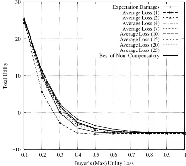
We expected that our other compensatory policy would show similar improvement to those of the previous subsection, when the number of distinguished situations increases. To this end, we use theLast 100deadline setting. Since there were three different parameters for distinguishing situations from each other, we increase the number of different cat-egories k on each from 1 to 10 and then 15, 20 and 25. Then some of the results are shown in figure 3. As can be seen, increasingk clearly improves the performance when
kis small, but with high kthere is no statistically signifi-cant improvement. This is because in our setting, most of the relevant patterns can be described with a relatively small number of distinctions. We therefore accept hypothesis 3.
−10 0 10 20 30
0.1 0.2 0.3 0.4 0.5 0.6 0.7 0.8 0.9 1
Total Utility
Buyer’s (Max) Utility Loss Expectation Damages
Average Loss (1) Average Loss (2) Average Loss (4) Average Loss (7) Average Loss (10) Average Loss (15) Average Loss (20) Average Loss (25) Best of Non−Compensatory
[image:7.612.331.523.538.709.2]The first policy to defeat all the non-compensatory ones consistently isAverage Loss(4).8 It will outperform all non-compensatory policies with the losses between0.3−0.6(at
p < 0.001level). Therefore we accept hypothesis 4 with Average Loss.
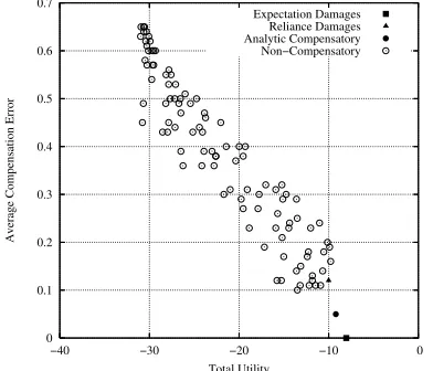
4.3.4 The Average Compensation Error
Finally, we investigate the relationship between average compensation error and the total utility. We calculated the average compensation errors and average total utility for all the policies. The preliminary results showed a clear correla-tion between the compensacorrela-tion error and performance when the fees were relatively low, but a larger variation when the fees were large (overall correlation−0.75). This is because the total average compensation error is not that good a metric if nobody ever decommits. In such cases, it hardly matters if the fee was1 or2.5. We can limit this effect by setting the maximum fee to be equal to the minimum one that al-lows nobody to ever decommit in a given contract. With this adjustment we then get figure 4, which shows a strong corre-lation, of−0.95, which is statistically significantly different from zero (atp < 0.001level). Compensatory policies are in the bottom right corner of the graph as one might expect from the above discussion.
0 0.1 0.2 0.3 0.4 0.5 0.6 0.7
−40 −30 −20 −10 0
Average Compensation Error
Total Utility
[image:8.612.71.267.366.534.2]Expectation Damages Reliance Damages Analytic Compensatory Non−Compensatory
Figure 4. Average Compensation Error and Total Utility.
The seller has no similar restriction on his loss and there-fore its losses can go higher and the effect described ear-lier is less pronounced (the correlation is−0.93without any adjustments). Both results give a clear indication that the average total utility is inversely related to the average com-pensation error and therefore we accept hypothesis 5.
5
Conclusions
In this paper, we showed that compensatory decommitment policies for contracts in electronic marketplaces can improve 8Already Average Loss(2) defeats non-compensatory policies when the loss is 0.4 or 0.5, but it loses to some policies when the loss is 0.2.
the welfare of the society and we gave two examples of such policies that work under incomplete information. We also showed how more accurate estimates for the losses improve the performance of both our policies. Moreover, we showed that in case of changing circumstances the performance of a market under a certain decommitment policy clearly depends on how accurately a policy compensates for the actual losses. For a designer of dynamic electronic marketplaces, the conclusions of this paper are as follows. First, decommit-ment policies can and do affect the performance of the mar-ketplace. Therefore a suitable decommitment policy should be a part of the overall design of any marketplace, where the parties’ preferences or circumstances can change after the contract has been entered into but before it is performed. Second, a compensatory policy is a serious contender for such policy if enough reliable information about the par-ties’ costs, valuations, preparations times and so on is readily available and can easily be obtained.
In future work, we extend the compensatory policies to cases in which the victims try to find substitute contracts to replace the ones they lose when their opponent decommits. Another direction of future work is to consider other effects that decommitment policies may have. Specifically, the law and economics literature has identified three key decisions, in which the decommitment fees play a role: the decision of whether or not to perform a contract (performance decision, the topic of this paper), but also whether or not to rely on the upcoming performance (reliance decision) and whether or not to enter a contract in the first place (contract decision).
References
[1] M. R. Andersson and T. W. Sandholm. Leveled commitment contracts with myopic and strategic agents. Journal of Eco-nomic Dynamics & Control, 25:615–640, 2001.
[2] J. H. Barton. The economic basis of damages for breach of contract.Journal of Legal Studies, 1(2):277–304, June 1972. [3] C. B. Excelente-Toledo, R. A. Bourne, and N. R. Jennings.
Reasoning about commitments and penalties for coordination between autonomous agents. In Proceedings of 5th Inter-national Conference on Autonomous Agents, pages 131–138, Montreal, Canada, 2001.
[4] P. Faratin, C. Sierra, and N. R. Jennings. Negotiation deci-sion functions for autonomous agents. International Journal of Robotics and Autonomous Systems, 24(3-4):159–182, 1998. [5] N. R. Jennings. Commitments and conventions: The founda-tion of coordinafounda-tion in multi-agent systems. The Knowledge Engineering Review, 8(3):223–250, 1993.
[6] T. D. Nguyen and N. R. Jennings. Managing commitments in multiple concurrent negotiations.Int. Journal of Electronic Commerce Research and Applications, 4(4):362–376, 2005. [7] T. Sandholm and V. Lesser. Advantages of a
leveled-commitment contracting protocol. InProceedings of the 13th National Conference on Artificial Intelligence, pages 126–133, Portland, OR, USA, 1996.