Interannual variability in the freshwater content of the
Indonesian-Australian Basin
Helen E. Phillips
CSIRO Marine Research, Hobart, TAS 7001, Australia.
Susan E. Wijffels
CSIRO Marine Research, Hobart, TAS 7001, Australia.
Ming Feng
CSIRO Marine Research, Floreat, W.A. 6014, Australia.
An average freshening of 0.2 psu, extending from 100oE to Australia, 25oS to Indonesia and down to 180 m depth, persisted for more than 3 years from 1999 to 2002. We map the anomaly using CTD profiles from Argo floats and suggest that the dominant forcing for the anomaly is surface freshwater flux over the Indonesian seas that is advected into the region. Using historical CTD data and surface freshwater flux reanalysis products we show that the Indonesian Australian Basin experiences strong interannual variability in upper ocean freshwater content and that the recent fresh event, a result of a long-lasting La Ni˜na, is unprecedented during the last 25 years.
1. Introduction
The Indonesian-Australian basin (IAB) receives fresh-water both through local strong wet-season precipitation associated with the Asian-Australian northwest monsoon of the Southern Hemisphere summer with weaker pre-cipitation over the rest of the year, and advectively via regional currents such as the Indonesian Throughflow (ITF) and South Java Current. Interannual variability in precipitation is strong: there is a precipitation deficit during the warm phase of ENSO (El Ni˜no) and an excess during the cold phase (La Ni˜na) [Ropelewski and Halpert, 1992, 1989; Haylock and McBride, 2001]. ITF strength also varies according to the phase of ENSO: stronger (weaker) throughflow during La Ni˜na (El Ni˜no) [Meyers, 1996].
La Ni˜na conditions persisted for an unusually long period at the end of the 20th century, from mid-1998 until early 2001. According to surface fresh-water fluxes from the NCEP DOE-AMIP II (NCEP)
[Kanamitsu et al., 2002] and ECMWF ERA-40 (ERA,
http://www.ecmwf.int/research/era) reanalyses, the ex-cess of precipitation integrated over this La Nina period was unprecedented over the reanalysis record (25 years, NCEP; 44 years, ERA). We now describe the impact of this massive freshwater flux on the upper thermocline waters of the IAB using in-situ observations from Argo profiling floats, supported by hydrographic and thermos-alinograph data.
Copyright 2005 by the American Geophysical Union. 0094-8276/05/$5.00
2. Data
Argo floats deployed by CSIRO, Australia, have been sampling the IAB since the end of 1999, returning CTD profiles every 10 days to a nominal depth of 2000 m. Fig. 1 shows float profile locations (pink) and contours of annual mean salinity from CARS2000 (CSIRO At-las of Regional Seas) on potential temperature surface
θ=22oC. The South Equatorial Current is seen as the in-creased meridional salinity gradient near 15oS, and the mean Indonesian Throughflow as the tongue of relatively fresh water adjacent to Indonesia. CARS2000 is a high-resolution climatology of the Australian region that accu-rately resolves large-scale and narrow coastal features in the Australian region [Ridgway et al., 2002]. Hereafter, the climatology, or mean, refers to the annual mean field of CARS2000.
Salinity data from the floats have been calibrated us-ing 7 high quality CTD surveys between 1989 and 2000, intercalibrated using WOCE I10 as the reference (Ta-ble 1). If the float conductivity ratio R at the coldest level measured exceeds meanRat that level in the CTD data by 3σ, then the float R profile is adjusted so that floatRequals CTDRat the deep level. This technique is extremely effective at correcting for sensor drift due to the great stability within the deep water masses (near
θ=3oC) in this region. This calibration is provided in real-time to the Argo global data centres.
Thermosalinograph (TSG) data collected and qual-ity controlled as part of the French “Observatoire de Recherche pour l’Environnement” dedicated to sea sur-face salinity (T. Delcroix, personal communication) is used to provide independent corroboration of sea surface salinity (SSS) variability between September 1999 and November 2002.
In Sect. 4 we relate ocean salinity to surface freshwater fluxes from the NCEP and ERA reanalyses and from meteorological stations on Cocos (12o11’21”S, 96o50’04”E) and Christmas (10o27’10”S, 105o41’15”E) Islands (Fig. 1). The Christmas Island precipitation (evaporation) P(E) record covers the period 1973-2002 (1972-1980) and the Cocos Island record covers 1901-2002 (1982-2003).
3. Mapping salinity anomalies
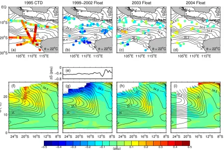
In the hydrographic data we see strong interannual variability in the upper ocean freshwater content of the IAB (Table 1). Relative to the climatology, 1989 was fresh, and 1992 and 1995 were salty over the upper 180 metres of the IAB. By 2000 the upper ocean had returned to fresh conditions. In 1995 there were 5 cruises and from these we construct a plan view (onθ=22oC) and zonally-averaged vertical section of salinity anomalies for this very salty period (Figs. 2a,f).
The spatial extent of the anomaly is revealed by plot-ting together all 3-monthly anomalies from the beginning of the record until the end of 2002 (Fig 2b). The re-gional coherence is striking with freshening in different 3 month blocks ranging from -0.02 to -0.42 psu with a mean and standard deviation of -0.19±0.1 psu. Zonally averaged, the fresh anomaly extends to approximately
θ=20oC throughout the southern part of the region, and to colder levels in the north where the thermocline is sharp and shallow (Fig. 2g). On pressure surfaces, the anomaly extends to a near-uniform 180 dbar at all lati-tudes. The largest salinity anomalies are in the south of the domain. Zonally and vertically averaged (0-180 m), the anomaly reaches a maximum of -0.37 psu near 18oS and is weakest near 10oS (-0.11 psu).
We tested the sensitivity of these results to the choice of climatology by repeating the calculations with the isopycnally-averaged climatology of Gouretski and Kolterman [Gouretski and Koltermann, 2004]. We find very similar results: the mean freshening onθ=22oC is -0.17±0.1 psu, the maximum freshening averaged over the upper 180 m of -0.36 psu occurs near 20oS, and the minimum is -0.1 psu near 8-10oS.
Near the end of 2002 the freshening begins to wane, and during 2004 the region becomes saltier than climatol-ogy. Figure 2c (2d) shows salinity anomalies onθ= 22oC
for 3 month blocks of float data sampled during 2003 (2004). The coherent, very fresh signal seen in Figs. 2b,g is replaced first by a mixture of fresh and salty anomalies (Fig. 2c,h), then by a return to generally salty conditions following the 2002/2003 El Ni˜no (Fig. 2d,i).
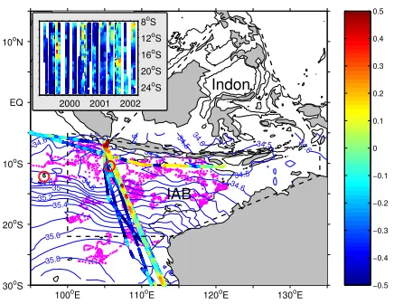
TSG data corroborates the upper ocean freshening we see in the float data between 1999 and 2002 (Fig. 1). Along the ship track passing through the centre of the Argo array, SSS anomalies relative to climatology of up to 2 psu are widespread. The time series of zonally av-eraged anomalies (100oE-120oE) south of 8oS(Fig. 1 in-set) is dominated by a fresh signal interrupted by bursts of salty anomalies. The mean meridional variation of salinity anomaly from September 1999 to September 2002 (Fig. 2e) shows a fresh anomaly at all latitudes, with an all-latitude mean of -0.42 psu and a standard deviation of 0.33 psu.
4. Freshwater Balance
NCEP and ERA reanalyses show strong interannual variability in surface freshwater flux northwest of Aus-tralia. Maps of monthly anomalies of P-E for both sets of reanalysis data show that the recent La Nina had the greatest impact on the Indonesian internal seas (Indon box in Fig. 1) and weaker positive anomalies over the IAB. Monthly anomalies are deviations from the 1979-2001 mean spatial distribution of P-E. A seasonal cycle was not removed because we relate the freshwater fluxes to ocean salinity from which we cannot remove the sea-sonal cycle. The intensity of rainfall rose somewhat above anomalies during non-La Ni˜na years. However, the prin-cipal contributor to enhanced P-E during 1999-2001 was the extension of the rainy season to 9 months (October-June). Runoff from land is included indirectly since the Indon and IAB boxes extend over land.
The contribution to upper ocean salinity change of the IAB and Indon freshwater inputs is estimated using a simple 1-D mixing model, neglecting advection. The salt balance equation when only the tendency and sur-face fluxes are considered can be written ∂S
∂t = ∂Fs
Sis salinity,Fsis vertical turbulent salt flux,tis time and
z is depth. Integrating vertically over the layer of depth
H that is influenced by surface fluxes, and neglecting vertical exchange through the base of the layer, salinity change is given by
∆S=−So(P−E)∆t
H (1)
where,Sois the surface salinity, equal to the vertically av-eraged salinity from the previous time step andP−Eis a time series of monthly anomalies. Initially,So=34.5 psu. From the Argo observations, H ≈ 180 m, in the main thermocline.
Salinity change due to the freshwater input in the In-don and IAB boxes are considered separately. The time for a parcel of water to transit from the Pacific Ocean to the Indian Ocean is about 1 year based on a core speed for the ITF of 10 cm s−1 and a path length of 3000 km. Transit time across the IAB is also about 1 year (SEC speed of 10 cm s−1, basin width of 2500 km). Argo data indicate that fresh anomalies persisted for a year after the end of the 1998-2001 La Ni˜na. Thus, to simulate the cu-mulative salinity change during transit time we integrate ∆Sover the previous year
Σ =1
τ
Z t
t−τ
∆Sdt, τ= 1 year (2)
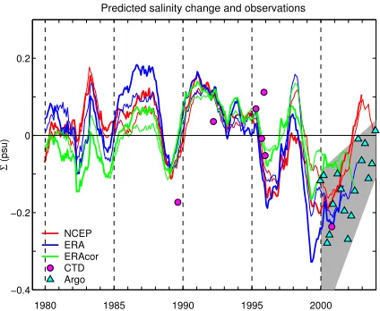
Σ due to Indon P-E (thin line) and due to the com-bined effect of IAB and Indon P-E (heavy line) are shown in Fig. 3 for NCEP (red), ERA (blue) and ERA-corrected (green). Σ due to Indon P-E is lagged by 1 year from that due to IAB P-E. Indon P-E is the dominant contributor to salinity change in the IAB. However during the salty mid-late 1980s and during the recent fresh event Σ had a large component due to IAB P-E. Predictions from each product are very similar during 1988-1995. Before and after this period they vary widely.
ERA is known to have excessive precipitation in the tropics resulting from a weakness of the humidity scheme used in the assimilation system Troccoli and K˚allberg [2004]. The ERAcor time series of Σ in Fig. 3 (green) uses ERA P with the global correction of Troccoli and K˚allberg [2004] applied.
Also shown in Fig. 3 are the mean salinity differences from climatology of the Argo data (triangles) and CTD (circles). For Argo each point represents the mean salin-ity difference in a 3 month period (JFM, etc.) averaged over the upper 180m of all profiles between 98oE-125oE, 28oS-8oS. For CTDs each point represents a mean anom-aly for the voyage over the upper 180 m of the same region. The sign and amplitude of the predicted salinity change from both freshwater products generally agrees well with the anomalies from the in situ data. During the fresh event, uncorrected ERA predicts the freshest anomalies which agree best with anomalies from Argo. Variability amongst in situ data points close in time is high. However, the data suggest that advection of fresh water from the Indonesian seas into the IAB is an impor-tant component of the upper ocean freshwater budget of the IAB.
5. Discussion
mean freshening of 0.2 psu over a 3 year period was the result of the unusually long-lived La Ni˜na of 1998-2001. During 2004 the IAB has returned to salty conditions fol-lowing the recent El Ni˜no. Hydrographic data from 1989 to 2000 provides evidence of strong interannual variabil-ity in upper ocean salinvariabil-ity in the region: fresh in 1989, salty in 1992 and 1995, fresh again in 2000. A simple salinity balance suggests that the dominant mechanism for interannual variability in upper thermocline salinity is the advection of salinity anomalies created by surface freshwater fluxes in the Indonesian seas into the IAB.
It is remarkable that despite the complexity of the IAB current systems, our simple mixing model and gross assumptions of residence times lead to predictions of salinity change in reasonable agreement with observed changes. Clearly there are exceptions such as in 1989 when the mean salinity anomaly from the JADE-89 cruise is -0.17 psu, considerably fresher than predicted by either flux product. This was a year dominated by strong La Nina conditions when the ITF was flowing strongly [ Mey-ers, 1996]. The large underestimate of predicted salinity change could be an indication that the spatial averag-ing of P-E underestimates forcaverag-ing delivered to the ITF jet itself. When the ITF is flowing strongly additional freshening from rainfall in the western Pacific may also be advected into the IAB. It is also possible that the reanalysis fluxes are biased low.
Rainfall across Indonesia in the reanalysis data is likely to be well constrained by the large number of rainfall stations there [Haylock and McBride, 2001]. In the IAB there are only 2 stations: Christmas and Cocos Islands. At Christmas Island, monthly anomalies of P are well represented in NCEP at the closest grid point, although minima are weaker than observed. Corrected ERA P un-derestimates both peaks and troughs. The uncorrected ERA P agrees best with the observations. Correlation coefficients and RMS differences (mm day−1) between reanalysis and observed P are 0.8/2.94, 0.72/3.15 and 0.62/3.94 for ERA, ERAcor and NCEP. At Cocos Island, there is little correlation between any product and obser-vations (corr. coef. <0.32). E has an amplitude of about a factor of 4 less than P and so variability in P-E is dom-inated by that of P. As far as we can tell, the reanalyses are representative of surface freshwater fluxes observed on Christmas Island, and by extension, in the IAB. The zonal-mean correction to tropical precipitation in ERA [Troccoli and K˚allberg, 2004] does not seem warranted in the IAB.
There is considerable scatter in the Argo observations. The two data points OND 1999 and JFM 2000, at the be-ginning of the Argo measurements when little data were available, are much less fresh than subsequent observa-tions and the predicobserva-tions (NCEP and ERA-uncorrected). As greater float coverage is achieved (mid 2000 - mid 2001) we obtain more consistency between float esti-mates. Halfway through 2001, several floats ceased op-eration, meridional coverage was again reduced, and the data points between JAS 2001 and JAS 2002 are quite scattered. In early 2003 we again achieved good merid-ional coverage and the scatter between observations was reduced. The shaded region in Fig. 3 highlights the con-vergence of Argo estimates in recent times. The mini-mum in salinity anomaly in OND 2001 may well be real and is seen to a smaller degree in the ERA uncorrected prediction.
salin-ity anomaly from the floats: a general trend of increas-ing salinity from a strongly fresh period through neutral to salty conditions. This study demonstrates that as the density of the Argo array approaches its target, Argo will provide a valuable tool to improve our understanding of regional and global freshwater balances and to validate surface flux products.
In future work we will undertake a full salinity bud-get for the IAB using a hindcast simulation from a global model with high-resolution (101o) in the Asian-Australian region. The fresh anomaly of 1999-2002 is clearly present in the hindcast. With this analysis we hope to gain a better understanding of the roles of advection and mix-ing in the arrival and departure of salinity anomalies in/from the IAB, and explore whether forcing may be-gin in the western Pacific. We will also investigate the mechanism by which the anomaly reaches 180 dbar, pos-sibly enhanced mixing in the Indonesian seas [Ffield and Gordon, 1992].
Acknowledgments. We thank the Captain and crew of many vessels who have deployed floats, including those from the Perkins Shipping Company, Peter Jackson for convincing the shipping companies to allow float deployments, Peter Man-tel for engineering improvements to the floats and foolproof de-ployment instructions, Alex Papij for supervision of engineer-ing improvements, and Bagus Hendrajana from Agency for Marine Affairs and Fisheries, Indonesia for deploying floats in Indonesia’s EEZ. This work was supported by the Australian Greenhouse Office and CSIRO.
References
Ffield, A., and A. Gordon, Vertical mixing in the Indonesian thermocline,J. Phys. Oceanogr.,22, 184–195, 1992. Gouretski, V. V., and K. P. Koltermann, WOCE global
hy-drographic climatology, Tech. Rep. 35/2004, Berichte des Bundesamtes f¨ur Seeschifffahrt und Hydrographie, 49pp, 2004.
Haylock, M., and J. McBride, Spatial coherence and pre-dictability of Indonesian wet season rainfall, J. Climate,
14, 3882–3887, 2001.
Kanamitsu, M., W. Ebisuzaki, J. Woollen, S. Yang, J. Hnilo, M. Fiorino, and G. Potter, NCEP-DOE AMIP-II reanalysis (R-2),Bull. Amer. Meteor. Soc., pp. 1631–1643, 2002. Meyers, G., Variation of Indonesian throughflow and the El
Ni˜no - Southern Oscillation, J. Geophys. Res.,101(C5), 12,255–12,263, 1996.
Ridgway, K. R., J. R. Dunn, and J. L. Wilkin, Ocean interpo-lation by four-dimensional weighted least squares - Appli-cation to the waters around Australasia,J. Atmos. Ocean. Technol.,19, 1357–1375, 2002.
Ropelewski, C. F., and M. S. Halpert, Precipitation patterns associated with the high index phase of the Southern Os-cillation,J. Climate,2, 268–284, 1989.
Ropelewski, C. F., and M. S. Halpert, Global and re-gional scale precipitation patterns associated with the El Ni˜no/Southern Oscillation,Mon. Wea. Rev.,5, 1606–1626, 1992.
Troccoli, A., and P. K˚allberg, Precipitiation correction in the ERA-40 reanalysis,Tech. Rep. 13, ERA-40 Project Report Series, 2004.
H. E. Phillips, CSIRO Marine Research, Hobart, TAS 7001, Australia. ([email protected])
S. E. Wijffels, CSIRO Marine Research, Hobart, TAS 7001, Australia. ([email protected])
−0.5 −0.4 −0.3 −0.2 −0.1 0 0.1 0.2 0.3 0.4 0.5
35.8 35.6
35.4 35.235 34.8
34.8 34.6
34.6 34.6
34.6
34.5 34.5
34.5
34.5 34.6
100oE 110oE 120oE 130oE
30oS
20oS
10oS
EQ
10oN
Indon
IAB
24oS
20oS
16oS
12oS
8oS
2000 2001 2002
Figure 1. Surface salinity anomalies (psu) from
thermosalinograph data (courtesy of T. Delcroix, IRD, France). Also shown, location of Argo profiles (pink), climatological salinity onθ=20oC (blue contours), loca-tion of Cocos and Christmas Islands (red circles, Cocos at left), and the two regions over which surface freshwa-ter fluxes are averaged (dashed boxes). Inset shows the temporal evolution of zonally averaged salinity anomalies from thermosalinograph
Voyage Start Date End date Location ∆S
JADE 89 30/7/1989 9/12/1989 IAB -0.17
JADE 92 17/2/1992 23/3/1992 IAB 0.04
F395 1/4/1995 22/4/1995 IAB 0.07
F895 13/9/1995 14/10/1995 IAB -0.01
I10 11/11/1995 28/11/1995 IAB 0.11
I02 2/12/1995 28/12/1995 8oS -0.05
[image:7.595.65.283.168.336.2]DOTSS 27/9/2000 11/11/2000 20-35oS, 100oE-Australia -0.24
Table 1. CTD data used in the study. ∆S is the mean
salinity difference from CARS2000 of all CTDs within 98o
E-125oE, 28oS-8oS, averaged over the upper 180 m. Negative
34.6 34.8
35 35.2
35.4
30oS 20oS 10oS
EQ
105oE 110oE 115oE
1995 CTD
θ = 22oC (a) 34.4 34.4 34.6 34.6 34.8 34.8 34.8 35 35.2 35.4
105oE 110oE 115oE
1999−2002 Float
θ = 22oC (b) 34.2 34.434.4 34.6 34.6 34.8 34.8 34.8 35 35.235.4
105oE 110oE 115oE
2003 Float
θ = 22oC (c) 34.2 34.4 34.4 34.6 34.6 34.8 34.8 34.8 35 35.2 35.4
105oE 110oE 115oE
2004 Float
θ = 22oC (d) −0.8 −0.4 0 ∆ S (psu) (e) 34.5 35 35 35.5 Θ ( oC)
24oS 20oS 16oS 12oS 8oS (f) 0 10 20 34.5 34.5 35 35 35.5
24oS 20oS 16oS 12oS 8oS
(g) 34.5
34.5
35
35 35.5
24oS 20oS 16oS 12oS 8oS (h)
34.5
34.5
35 35.5
24oS 20oS 16oS 12oS 8oS (i)
[image:8.595.60.499.66.360.2]−0.5 −0.4 −0.3 −0.2 −0.1 (psu)0 0.1 0.2 0.3 0.4 0.5
Figure 2. Salinity anomalies relative to CARS during 1995 from WOCE CTDs, during the fresh event of 1999-2002
−0.4 −0.2 0 0.2
Σ
(psu)
Predicted salinity change and observations
1980 1985 1990 1995 2000
[image:9.595.68.280.64.238.2]NCEP ERA ERAcor CTD Argo
Figure 3. Predicted salinity change of the upper 180