Eigenvalue Problems
C hristopher R obert Dun
March, 1995
S ta te m e n t o f C o n te n t
Part of Chapter 3 of this thesis has been submitted for publication, and repre sents joint work with Anderssen1. A paper based on Chapter 5 is also in prepara tion with Anderssen.
Unless otherwise stated in the text, the remainder of this thesis is my own work.
1C.R. Dun, R.S. Anderssen, “A modification of Paine’s algebraic correction method for inverse Sturm-Liouville problems” Submitted for publication
I would like to thank my supervisor. Bob Anderssen, for giving me a good problem, and making me own it. His supervision and suggestions have been in valuable throughout this Ph.D. I would also like to thank Frank de Hoog for his many helpful comments.
Thanks must also go to Markus Hegland, Steve Roberts and Mike Osborne for proof-reading parts of this thesis. Their advice improved the clarity of the thesis, and ironed out a few bumps.
Special thanks go to Kit for her love and support, especially in the last three months.
Eigenvalue problems, in their many forms, play an important role in many branches of applied mathematics. One of the reasons for this is that eigenvalue problems model vibrating systems, with the eigenvalue determining the frequencies of vibra tion.
The natural approach to the eigenvalue problem is to calculate the eigenval ues from a knowledge of the underlying system. This is known as the forward problem. In many important applications in physics and medicine, the details of the underlying system are unknown, but the vibrations produced bv the system can be measured. The problem is to determine information about the underlying system from the vibrations it produces. In terms of the eigenvalue problem, this is equivalent to reconstructing the underlying system from the eigenvalues. This is known as the inverse problem.
The eigenvalue problem considered in this thesis is the Sturm-Liouville problem in potential, or Liouville normal, form
These two problems model, for example, the vibrations of a stretched string and a thin membrane, respectively. In each case, the eigenvalues and corresponding eigenfunctions are denoted by Ak, and uk, respectively. In addition, q denotes the potential.
Both the forward and the inverse formulations of the one-dimensional Sturm- Liouville problem have been extensively studied. One of the main topics covered by this thesis is numerical techniques for solving the inverse problem. In particular, a method due to Paine [68], based on the algebraic correction methodology [70], is considered in detail. A modification of this method is proposed, and is shown to give improved results. It is established that the potential reconstructed using the modified method converges to the actual potential, in the L2 sense, as the discretisation becomes finer.
u"k(x ) + q{x)uk{x) = AkUk(x) , x £ (0,7r) Uk(0) = 0 = uk(7r),
and its generalisation to two dimensions
- A u k(x, y) + q{x, y)uk(x, y) = Akuk{x, y) uk(x,y) = 0
{x,y) £ Q, (x, y) £ dQ .
two-dimensional problem is considerably more complex than the one-dimensional problem. The behaviour of the eigenvalues and corresponding eigenfunctions of the two-dimensional problem is not as well understood, and is more difficult to control, than in the one-dimensional problem.
In this thesis, numerical methods for calculating the eigenvalues of the two- dimensional eigenvalue problem are considered. It is found that, although standard methods may be used, they require large amounts of computer time and storage if long sequences of uniformly accurate eigenvalues are required.
The algebraic correction methodology, due to Paine, de Hoog and Ander- ssen [70], is extended to calculating the eigenvalues of the two-dimensional eigen value problem. It is shown that, providing the ordering of the eigenvalues can be controlled, the algebraic correction is a fast, efficient, method for calculating long sequences of uniformly accurate eigenvalue approximations.
The motivation for calculating long sequences of eigenvalues of the two-dimen sional problem is their use as data for the study of algorithms for the solution of the corresponding inverse problems. To test algorithms for solving inverse prob lems, a known potential is chosen and its eigenvalues determined. The algorithm for solving the inverse problem is applied to the resulting eigenvalues, and the potential reconstructed. The reconstructed potential can then be compared to the given potential, to assess the performance of the algorithm. The absolute error in the approximations to every eigenvalue must be small, since the inverse prob lem is improperly posed. Thus, small errors in the given eigenvalues can lead to large errors in the reconstructed potential, which makes it difficult to evaluate the reconstruction algorithm.
S t a te m e n t o f C o n te n t i
A c k n o w le d g e m e n ts ii
A b s tr a c t iii
1 I n tr o d u c tio n 1
1.1 Introduction to Eigenvalue P ro b le m s ... 1
1.2 Background T h eo ry ... 3
1.2.1 The Forward Problem ... 4
1.2.2 The Inverse P ro b le m ... 5
1.3 Historical Overview... 7
1.4 Summary of the T h e sis... 10
2 T h e O n e -D im e n sio n a l A lg eb ra ic C o rrectio n 13 2.1 In tro d u ctio n ... 13
2.2 The Rayleigh-Ritz Discretisation ... 14
2.3 The Algebraic Correction M e th o d ... 16
2.4 Extensions to the Algebraic Correction M e t h o d ... 19
2.5 Numerical R esults... 23
3 T h e O n e -D im e n sio n a l I.E .P . 26 3.1 In tro d u ctio n ... 26
3.2 Review of Methods for the One-Dimensional I.E.P... 29
3.2.1 The Rayleigh-Ritz Method for the Solution of the One-Di mensional Inverse Eigenvalue Problem ... 30
3.2.2 Paine’s Method for the Solution of the Inverse Problem . . . 32
3.2.3 Pirovino’s Method for the Solution of the One-Dimensional Inverse Eigenvalue P r o b le m ... 37
3.3 A Modification of Paine’s M e th o d ... 39
3.4 A Convergence Analysis of the Modified M eth o d ... 45
3.5 Numerical Im plem entation... 58
4 C a lc u la tin g T w o -D im e n sio n a l E ig en v a lu es 65
4.1 In tro d u ctio n ... 65
4.2 Multigrid with Ritz P ro je ctio n s... 69
4.2.1 Introduction to Multigrid ... 69
4.2.2 Calculating the Eigenvalues of a Two-Dimensional Differen tial Operator using Multigrid ... 76
4.2.3 The Ritz Projection ... 82
4.2.4 Numerical Results ... 83
4.3 The Lanczos Method and Extrapolation ... 84
4.3.1 Introduction to the Lanczos Method ... 84
4.3.2 E x trap o latio n ... 88
4.3.3 Numerical Results ... 94
5 T h e T w o -D im e n s io n a l A lg eb ra ic C o rrectio n 98 5.1 In tro d u ctio n ... 98
5.2 Algebraic Correction on the Separated P o te n tia l... 99
5.3 Algebraic Correction in Two D im ensions...109
5.4 Non-Separable Algebraic Correction...114
6 T h e T w o -D im e n s io n a l I.E .P . 118 6.1 In tro d u ctio n ... 118
6.2 Review of Two-Dimensional M eth o d s...121
6.3 Algebraic Correction and the 2D I.E.P... 126
6.3.1 The Two-Dimensional Modified Method ... 128
6.3.2 Pirovino's Method in Two D im en sio n s... 130
I n tr o d u c tio n
1.1 I n t r o d u c t i o n to E ig e n v a lu e P r o b le m s
Eigenvalue problems, in their many forms, play a significant role in most areas of applied mathematics. One of the reasons for their importance is the fact that they are used to model oscillating systems.
Periodic and vibrational movement can be seen everywhere in life. From the movement of atoms and electrons to the orbits of planets, oscillating systems are present. If the periodic components are extracted from the mathematical mod els used to represent the oscillating systems, then one is left with an eigenvalue problem. In such situations, the eigenvalues correspond to the frequencies of the vibrations.
As a simple example of this process, consider the transverse vibrations of a one dimensional stretched string. Suppose the string has length L, is under constant tension T, and has a non-constant linear density p. Then the movement of the string is governed by the simple wave equation [26, p. 287]
d2u(x, t) 2d2u(x,t)
dx? = C 9C ’ (11)
where c2 = p(x)/T. It will be assumed that the string is fixed at the end points, so that the boundary conditions take the form
u(0, t) = 0 = u ( L, t) , for all t > 0.
Now, suppose the string is vibrating in a normal mode so that u has the form u(x, t) = X(x)(acosujt + b sin cut) .
Writing the solution u(x, t) as a function in x, multiplied by a function in t, is the principal assumption required for the separation of variables technique. Substitut ing the above form for the solution into (1.1), and applying separation of variables,
determ ines the eigenvalue problem
X "(x ) + Xp(x)X(x) = 0 , x E (0, / ) ,
A (0) = 0 = X ( L) . (1.2) N otice th a t separation of variables has also been applied to the boundary con ditions. T he param eter A := u r / T is introduced by the separation of variables condition, and corresponds to an eigenvalue of (1.2). Thus, the eigenvalues of (1.2) determ ine the frequencies of vibration of the string.
V ib ratin g strings are not the only source of eigenvalue problems. An im p o rtan t application of eigenvalue problems in physics is the one-dim ensional Schrödinger equation. A form ulation of this is given by [24, 74]
hi~
- “ - 0 + (V(x) - E)tjj = 0 , (1.3)
where i(j(x) is the wave function associated with the particle being modeled, V(x) is the potential field surrounding the particle, and E is its energy level. The mass of th e particle is given by m, and h = h/27T, where h is Planck's constant. In this application, the eigenvalue, E, corresponds to the energy of the particle.
As th e above examples show, eigenvalue problems come in a wide variety of forms, and model m any different processes. However, m any such problem s can be in terp reted as a special case of some canonical system. By studying this system, results can be obtained which are applicable to a wide variety of problems.
E quations (1.2) and (1.3) are both special cases of the canonical Sturm -Liouville eigenvalue problem, which is given by [8],
~ (^p(y)-^Vk(y)j + r(y)vk{y) = Xkw{y)vk{y) , y E (0, tt) , a v k(0) + ß — vk(y) = 0 ,
dy
7Vk(ir) + 5 — vk(y) dy
(1.4) y=o
= 0
y=7T
The problem (1.4) is regular if p and w are strictly positive on [0,7r], r, y E C[0 , 7r], and p E C ^O ,^]. It will be assumed throughout this thesis th a t a regular Sturm - Liouville problem is being studied.
T he canonical form (1.4) is quite general, and can often be simplified. For example, it can, under suitable regularity, be reduced to th e Liouville norm al form
- u k (x) + q(x)uk(x) = Xkuk{x) , x E (0, 7 r), ' a*uk(0) + ß u k{0) = 0 ,
7*ufc(7r) + ^4(71-) = 0 .
The transformation which affects this change is known as the Liouville transforma tion [26, p. 292]. Notice that the eigenvalues in (1.5) are identical to the eigenvalues in (1.4). Since the domain of both problems are the same, the transformation leaves the eigenvalues unchanged. In general, the eigenvalues of the transformed problem would be multiplied by a constant [26, p. ?]. Notice that the coefficients in the boundary conditions are affected by the transformation, although the boundary conditions of (1.5) have the same form as (1.4).
The problem (1.5) is said to be in potential form, with the function q(x) defining the potential. The reason for this is that the equations (1.5) model systems acting under a potential. For example, the Schrödinger equation (1.3) has the form (1.5), with the potential field V{x) playing the role of q(x).
The one-dimensional eigenvalue problem above can be generalised in many ways. Problems with higher order derivatives may be considered [61, 62, 34], and problems with non-linear dependence on the eigenvalues [25. 79, 8]. The generalisation which will be examined in this thesis is the eigenvalue problem in a higher dimension. As an example of this, consider the application of the separation of variables technique to the wave equation modelling the vibrations of a two-dimensional rectangular membrane. If this membrane is fixed along its boundary, the associated eigenvalue problem takes the form
where A denotes the usual Laplacian operator. Again, the eigenvalues Afc deter mine the frequencies of vibration of the membrane. Here, ft denotes the domain of the problem, in this case a rectangle. Although, in theory, any shaped domain may be considered, it will be assumed throughout the rest of this thesis that the two-dimensional eigenvalue problem is defined on a rectangle. This simplifies the problem significantly. For example, under appropriate conditions on the potential, separation of variables can be applied to (1.6) to reduce the problem to two, decou pled, one-dimensional problems. This is an important feature of this formulation, and will be extensively exploited.
The focus of this thesis is the one-dimensional Sturm-Liouville problem in po tential form, and its two-dimensional analogue (1.6). Both the forward and inverse problems associated with these systems will be examined. A definition of the for ward and inverse problems for the systems (1.5) and (1.6) will be given in the next section, along with a brief summary of the relevant theory for each problem.
1.2 B a c k g r o u n d T h e o r y
Many problems in mathematics may be categorised as either forward or inverse problems [15, p. 2]. Forward problems tend to be well-posed, and numerically
stable solutions can be found relatively easily. Inverse problems tend to be im properly posed [15, p. 14], which complicates the process of finding a numerical solution.
Both forward and inverse eigenvalue problems are examined below. For sim plicity, the definitions are given for the one-dimensional eigenvalue problem only. The concepts extend naturally to two, and higher, dimensions.
Because of their importance, eigenvalue problems have been extensively stud ied. Some basic theory concerning the forward and inverse problems, for both the one and two-dimensional problem, is included along with the definitions.
1 .2 .1 T h e Forw ard P r o b lem
The forward problem for the eigenvalue problem (1.5) is defined as follows. Given a potential q{x), satisfying certain regularity, and boundary data a and 3, determine the set of real values Ak such that, corresponding to each Afc, there exists a non trivial solution Uk{x) of (1.5).
This is the natural way of thinking about a Sturm-Liouville problem. Given the problem, determine the answers. The theory for this case is extensive [26, 57, 74]. It is known that if the potential is piecewise continuous, then there exists a countably infinite set of simple eigenvalues, with no finite accumulation point [31]; i.e.<I>.,
Ai < A2 < • • • Xk '30 as k —> oc.
As k increases, the separation between the eigenvalues increases. This can be seen from the asymptotic formula for the eigenvalues. Fix [31], in 1967, showed that for q € C L[0,7r]
Xk = k2 + — [ q(x)dx + 0 ( k~2) . 7r Jo
More recently, Pöschel and Trubowitz [72] have shown that for q e L2(0,7r) l
rn
Xk = A:2 -I— / q(x)dx + ^2( n ) . 7T Jo
The notation £2(n) has the following interpretation. If {an} and {ßn} are sequences of real numbers, then a n = ßn + l 2{ri) is equivalent to a n = ßn + yn, where £ n>0 72 < oo. Asymptotic formulas, such as those above, are used to prove uniqueness theorems for inverse eigenvalue problems [65].
Much less is known about the two-dimensional eigenvalue problem (1.6). For q E L°°(0,7r), there exists a countably infinite set of eigenvalues satisfying
Ai < A2 ^ A3 • • • Afc —y00 as k —y00.
One of the main difficulties encountered with two-dimensional eigenvalue problems is that the eigenvalues are not guaranteed to be distinct. For any given potential, it is possible that multiple, or nearly multiple, eigenvalues may be present. This makes calculating asymptotic formulae difficult, since the small separation between eigenvalues can give rise to small divisors in the asymptotic formulae [65]. Recently, Hald and McLaughlin [43] determined asymptotic expansions for a dense subset of eigenvalues and eigenfunctions of (1.6). These results have important implications for the inverse formulation of the eigenvalue problem. This will be discussed further in the next section.
Many of the numerical methods used to calculate eigenvalues for the one dimensional problem can be extended to two-dimensions. However, less work has been done on the validity of such methods in generating uniformly valid approxi mations to the eigenvalues of (1.6) [8, p. 26]. Knobel and McLaughlin [53] use a Rayleigh-Ritz method, with Legendre basis functions, to determine accurate eigen value approximations for the two-dimensional problem. Direct discretisation can also be extended to two dimensions. It will be shown in Chapter 5 that the alge braic eigenvalues resulting from this method are non-uniform approximations to the required differential eigenvalues. The main focus of Chapter 5 is the extension to two dimensions of the algebraic correction method. This method overcomes, to some extent, the non-uniformity of the algebraic eigenvalues.
1 .2 .2 T h e In v erse P r o b lem
The inverse problem for the one-dimensional eigenvalue problem (1.5) is more dif ficult to formulate than the forward problem. Depending on the situation, and the sort of data available, different formulations are appropriate. The most general definition of the inverse problem is the following. Given spectral data, Afc, corre sponding to the problem (1.5), determine the potential, q(x), and the boundary data a and /?, which can generate the given spectrum.
This formulation is less intuitive than the forward problem. In a sense, the answers are given, and the problem must be determined. Inverse problems tend to be improperly posed [15, p. 14]. Intuitively, the reason for this is that the equations governing the system are usually derived in the context of the forward problem. The equations are formulated in such a way that the forward problem is well-posed. However, such a formulation does not guarantee that the inverse problem will also be well-posed.
are known a priori. This simplifies the formulation considerably. For the inverse problems considered below, it will always be assumed that the boundary conditions are known.
Another difficulty in formulating the inverse problem is deciding what regularity may be assumed for the reconstructed potential. If too much regularity is imposed, it may be difficult to prove existence of the potential. If the potential is allowed to be too general, then proving uniqueness may be difficult.
There are three important questions which must be answered to completely solve any inverse problem. They are:
1. Existence. Under the conditions of the problem, does a solution exist, satis fying all the required properties?
2. Uniqueness. If a solution to the problem exists, is it unique within the class of prescribed solutions?
3. Reconstruction. If the solution exists and is unique, how can it be recon structed from the given data in a suitable manner?
The first two conditions correspond to two of the requirements for a well-posed problem, in the sense of Hadamard [49]. It is usually the third requirement, con tinuous dependence on the given data, which fails for inverse problems.
The inverse formulation of the Sturm-Liouville problem (1.5) has been exten sively examined. For this particular problem, each of the above questions have been answered satisfactorily. The history of the development of the theory for inverse problems will be discussed in the next section.
The approach taken to prove existence and uniqueness of the inverse eigenvalue problem is to find a “near-by” problem for which the solution is known [34, Ch. 9]. The known problem must be “near-by” in the sense that the eigenvalues of the given problem and the reference problem are asymptotically the same. An integral equation is then defined which relates the two problems. Existence and uniqueness follow from the properties of the integral equation [34, Ch. 9]
This concept of a near-by problem is also used in analytic reconstruction meth ods for the unknown potential [34, 63]. Many numerical reconstruction algorithms are also formulated around a near-by problem. For example, Hald [40] considers a reconstruction technique based on the Rayleigh-Ritz method. Hald’s reconstruc tion works because the basis functions used in the Rayleigh-Ritz iterations are chosen to be the eigenfunctions of a near-by problem. A suitable reference prob lem is also crucial in the reconstruction procedure based on the algebraic correction discussed in Chapter 3.
since the null-potential must be “near-by” to the given problem in the sense defined above.
The two-dimensional inverse eigenvalue problem has not been as well studied. The questions of existence, uniqueness and reconstruction have only been partially answered. A survey of relevant work will be presented in the next section.
Obtaining theoretical results for the two-dimensional inverse eigenvalue prob lem is significantly more difficult than for the one-dimensional problem. The m ath ematical structure of the two-dimensional eigenvalue problem is more complex than the one-dimensional problem.
One of the major difficulties encountered in reconstruction methods for the two- dimensional inverse eigenvalue problem is the behaviour of the reference problem. As in the one-dimensional methods, the reference problem is normally taken to be the null-potential system, q(x, y) = 0. However, the two-dimensional null-potential system, on the rectangle 17, is likely to have multiple or nearly multiple eigenvalues. This introduces several difficulties. Firstly, as mentioned in the previous section, the small differences between the eigenvalues can lead to small divisors in the asymptotic expansion of the eigenvalues. This means that the standard uniqueness and existence proofs in one dimension cannot easily be extended to two dimensions.
Another difficulty posed by multiple eigenvalues in the spectrum of the refer ence problem is the ordering of the given eigenvalues. Because of the additional structure of the two-dimensional problem, the ordering of the eigenvalues becomes important. One way of determining an appropriate ordering is to consider the eigenvalues of the reference problem. If there are multiple eigenvalues in the spec trum of the reference problem, then assigning an ordering to the given eigenvalues becomes ambiguous.
The first difficulty has been addressed by Hald and McLaughlin [43]. The details of how they overcome this difficulty will be given in the next section. A technique for dealing with the second difficulty will be discussed in Chapter 5.
1.3 H is to r ic a l O v e rv ie w o f t h e O n e a n d T w o - D im e n s io n a l E ig e n v a lu e P r o b le m s
The Sturm-Liouville problem was formulated, by both Sturm and Liouville, in a series of papers published in 1836-37 [56]. The formulation of the problem first considered was
p{a) — - hvk(a) = 0 ,
The main focus of the study of differential equations at this time was on obtaining analytic solutions. Sturm and Liouville found that no suitable analytic solutions could be found for the above problem. Thus, in a move which characterised the changing attitudes of the times, they considered properties of the solutions which could be determined from the equations. Most importantly, they strove to prove existence of solutions, without actually constructing them.
The formulation of Sturm-Liouville theory opened up a new branch of mathe matics. The generalisations of this theory led to singular problems (first studied in the form of the Bessel equation), higher dimensional problems, and ordinary differential equations with multiple parameters.
The development of a general theory of integral operators introduced a new approach to the Sturm-Liouville theory. The correspondence between the spectral theory for integral and differential operators was established using Green’s func tions. This correspondence has been important in the development of the theory for the inverse problem.
Sturm-Liouville theory has reached a significant level of sophistication. The problem is now most often formulated in the context of operators on Hilbert spaces. In this setting, quite general theorems can be proved [57].
The inverse problem was first studied by Ambarzumian [1] in 1929. He consid ered the problem
-u"k(x) + q(x)uk(x) = AkUk(x) , x G (0, n) , *4(0) = o = uk{7T) .
Ambarzumian [1] showed that, if Xk = /c2, and the potential is suitably small, then q(x) = 0. This was the first attempt to answer the question of uniqueness (question 2 in Subsection 1.2.2 above) of the inverse problem.
The fundamental paper in the area of inverse Sturm-Liouville problems was published by Borg [17] in 1946. Borg considered the question of uniqueness for the problem (1.5). For a potential q(x) G L2(0,7t), Borg found that the full spec trum is not enough to guarantee the uniqueness of the reconstructed potential. He found that extra information about the problem is required. This informa tion may take the form of another spectrum, corresponding to a different set of boundary conditions, or the normal derivatives of the eigenfunction evaluated on the boundary [72].
Instead of using more boundary data, Borg showed that it is possible to impose further regularity on the potential to obtain uniqueness with one full spectrum. For example, consider the eigenvalue problem
—uk(x) + q{x)uk(x) = AkUk(x) , x 6 (0,7r), Uk(0) = 0 = Uk(n) ,
assumed to be symmetric in the domain of interest; i.e.,
q(Ti - x) = q(x) , x £ (0,7r) , (1.8) then this is sufficient regularity to ensure uniqueness of the reconstructed potential. The initial results obtained by Borg have been extended and simplified by many authors [42, 46, 47, 54]. In particular, Hochstadt [46, 47] considered to what extent the potential could be reconstructed, given incomplete data.
Gel’fand and Levitan [33], in 1951, considered the question of existence. They found that under Borg’s conditions a solution to the inverse problem exists. Given a sequence of numbers as data, Gel’fand and Levitan showed what conditions the data must satisfy for it to correspond to the spectrum of some potential. Gel’fand and Levitan also showed how to reconstruct the potential from the given data. Unfortunately, their method is cumbersome to implement numerically.
A significant amount of work has been done on the question of reconstruction. McLaughlin [63] has reviewed some analytic techniques for reconstructing the po tential from eigenvalue data. Numerical methods for reconstructing the potential from finite data have also been considered extensively [13, 30, 40, 55, 68, 71]. Nu merical techniques for reconstructing a potential from eigenvalue data reduce the given problem to a finite dimensional one. This step introduces several difficulties. For example, the uniqueness of the reconstructed potential cannot be guaranteed because of the reduced amount of data. Additional assumptions must be placed on the problem to overcome this difficulty. Another difficulty is ensuring that the given data for the continuous problem is consistent with the data required for the finite dimensional problem. This difficulty is discussed further in Chapter 3.
The generalisation to higher dimensions of the inverse Sturm-Liouville problem has only recently been considered. The higher dimensional eigenvalue problem has a more complex structure, which makes proving general theorems challenging.
The first result in this area was obtained by Nachman et al. [66] in 1988. They showed that the full spectrum of (1.6) is again insufficient to guarantee the uniqueness of the reconstructed potential, and that additional information, in the form of another spectrum corresponding to Neumann boundary conditions, or the values of the normal derivative of the eigenfunctions evaluated on the boundary, is required for uniqueness.
The questions of existence of a solution, and what conditions the given data must satisfy to correspond to the spectrum of some potential, have not yet been answered. The question of reconstruction is also only partially answered.
their method to fail. This difficulty with multiple eigenvalues is a fundamental challenge for the two-dimensional inverse eigenvalue problem, and limits the ap plicability of extending one-dimensional methods to two-dimensions.
Hald and McLaughlin [43] have developed a reconstruction method for the re lated inverse nodal problem. In this formulation the data are not the eigenvalues, but the nodal lines of the corresponding eigenfunctions; i.e., the lines in the do main Q along which there is no vibration. Although this is a different problem, it is quite closely related to the inverse eigenvalue problem. In particular, Hald and McLaughlin need to control the behaviour of the eigenvalues to prove the unique ness of their method. Hald and McLaughlin [43] overcome the difficulty of multiple eigenvalues in the spectrum of the null-potential system by choosing special rect angles, and limiting consideration to those eigenvalues which are sufficiently well separated. By imposing these restrictions, they were able to prove uniqueness for their problem, and show that their reconstructed potential converged to the true potential as the discretisation became finer. So far, no actual numerical imple mentation of Hald and McLaughlin’s method has been made. The implementation of their method is made more challenging by the strict conditions which must be imposed to prove uniqueness and convergence. It is possible that in a numerical scheme, some of these conditions could be relaxed.
1.4 S u m m a r y o f t h e T h e s is
The remainder of the thesis has the following format.
The one-dimensional algebraic correction is reviewed in Chapter 2. Several extensions to the original proposal have been made, primarily by Andrew [5, 7], and Andrew and Paine [10, 11]. These extensions consider different boundary con ditions for (2.1), and different methods for discretising the differential operator. Andrew [4] briefly considers the extension of the algebraic correction to two di mensions, but notes that it is significantly more complex than the one-dimensional algebraic correction.
In Chapter 3, the one-dimensional inverse eigenvalue problem is examined. Sev eral methods for solving the problem are discussed. Two of the methods, Paine’s method [68] and Pirovino’s method [71] are based on the one-dimensional alge braic correction. Paine’s method is examined in detail, and a modification of the method, which gives improved results, is derived. An L 2 convergence result is obtained for this method, although numerical results suggest that the convergence may actually be L°°.
Two standard methods for calculating approximations to the eigenvalues of a two-dimensional differential operator are considered in Chapter 4. The first of these methods is a multigrid method based on a Ritz subspace iteration. The basic multigrid algorithm is described, and then extended to the non-linear problem of determining the eigenvalues of (1.6). The Ritz projections are described and some numerical results obtained.
The second method examined is the Lanczos method. The code for this method was taken from the MESCHACH library of numerical routines in C [78]. To obtain highly accurate estimates of the eigenvalues, extrapolation was applied to the ap proximations obtained using the Lanczos method. Using extrapolation, approxi mations to the eigenvalues accurate up to order-/?4 were obtained.
The main point of Chapter 4 is that although standard methods can be used to calculate the eigenvalues of a two-dimensional differential operator, in practice these methods can cause some difficulties. In general, calculating a long sequence of uniformly accurate eigenvalues can involve significant computing time and storage.
In Chapter 5, the extension to two dimensions of the algebraic correction methodology is considered. To simplify the problem, it is assumed that the bound ary of the domain is a rectangle, and that the two-dimensional potential q(x, y) is separable; i.e., it satisfies
q{x,y) =p{x) + r{y).
The advantage of imposing this assumption is that separation of variables may be applied to (1.6) to reduce it to two, coupled, one-dimensional problems, each having the form (1.7). The one-dimensional theory reviewed in Chapter 2 can then be applied. Recombining the eigenvalues of the one-dimensional problems, to give the two-dimensional eigenvalues, gives some insight into the behaviour of the eigenvalues of the two-dimensional problem. The key observation made here is that the ordering of the two-dimensional eigenvalues is crucial.
Based on this observation, a fully two-dimensional algebraic correction is de fined. To make this algebraic correction work, care must be taken with the order ing of the eigenvalues. The two-dimensional algebraic correction is extended to the case where the potential q(x, y) is not separable. In this situation, the ordering of the eigenvalues is unknown. To overcome this difficulty, it is assumed that the potential is a perturbation of a known, separable potential. The ordering of the eigenvalues of the separable potential can then be applied to the eigenvalues of the non-separable potential.
T he inverse problem for the two-dimensional eigenvalue problem (1.6) is con sidered in C h ap ter 6. Several m ethods, most of which are extensions of one dim ensional m ethods, are discussed. Due to the additional complexity of the two- dim ensional eigenvalue problem, each of these m ethods suffers from some lim ita tions.
T he generalisation of the modified P aine’s m ethod, and Pirovino’s m ethod, to two dim ension, is discussed. There are several difficulties which m ust be faced in order to use the two-dimensional algebraic correction to solve the inverse problem.
T he key to the success of the modified m ethod, and Pirovino’s m ethod, in one dim ension is the following observation. Given N algebraic eigenvalues, exactly N unknow ns can be reconstructed from this data. Thus, the crucial step is d eter m ining discretisations of the problem which have the same num ber of unknowns as d ata. T he modified m ethod and Pirovino’s m ethod approach this constraint in different ways. The modified m ethod considers all the given d a ta, and con stru c ts a discretisation having N unknowns. Pirovino’s m ethod uses the stan d ard discretisation, which has only n = yv+i unknow ns.1 Instead of extending the discretisation, Pirovino restricts the given d a ta to n eigenvalues.
It is found th a t a straightforw ard generalisation to two dimensions of the m od ified m ethod fails to give a discretisation with the required num ber of unknowns. Several ways of overcoming this difficulty are briefly discussed.
Pirovino’s m ethod generalises directly to two dimensions. The stan d ard dis cretisation of the problem may be used, and then the given d a ta restricted to the num ber of unknowns. A formal extension to two dimensions of Pirovino’s m ethod is derived.
T h e O n e-D im en sio n al A lgebraic C o rre c tio n
2.1 I n tr o d u c tio n
Except under special conditions, the solution of the forward problem for the one dimensional Sturm-Liouville problem must be determined numerically. To do this, some sort of discretisation must be imposed on the problem. In general, the dis cretisation leads to a corresponding matrix eigenvalue problem which can be solved using a standard method.
A few subtle difficulties are associated with this approach. The standard method of discretising the problem is to approximate the eigenfunctions in some way. The difficulty with this approach is that the eigenfunctions, corresponding to the high order eigenvalues, are very oscillatory. Thus, the discretisation can often fail to approximate the higher eigenfunctions accurately. In this case, the high order eigenvalues of the matrix problem bear little resemblance to the differential eigenvalues [8]. As the breakdown in the approximation can be quite rapid, deter mining long sequences of uniformly accurate eigenvalues is more challenging than simply applying a standard discretisation to the problem.
There are several ways of overcoming this difficulty. Discretisations exist which take into account the oscillatory nature of the eigenfunctions, and thus give good approximations to the high-order eigenvalues [40]. Unfortunately, these discreti sations often lead to dense matrix representations of the problem. An example of such a discretisation is given in the next section.
An alternative approach is to approximate the coefficients of the problem (in this case the potential q(oc)). Canosa and Gomes de Oliveira [24] approximated the potential by a piecewise constant function. On each constant region, the Sturm-Liouville problem can be solved exactly. The eigenvalues are determined by requiring that the solution is continuous on the whole domain.
Pruess [73] extended this idea by approximating the potential by piecewise polynomials. Pruess showed that this approximation preserves the asymptotics of the problem, and hence uniform eigenvalue estimates can be calculated. Un fortunately, the Sturm-Liouville problem can no longer be solved exactly on each
region of the domain. Pruess calculated the eigenvalues of the approximate Sturm- Liouville system using a shooting method. He noted that a polynomial potential lends itself to numerical integration. Thus, the initial value problem, associated with the Sturm-Liouville problem, was integrated numerically. The eigenvalues were determined by enforcing the second boundary condition. Pruess [73] showed that this method is consistent, and that the approximations converge to the actual eigenvalues.
Paine and de Hoog [69] noted that the method proposed by Pruess is inefficient to implement, unless piecewise constant functions are used to approximate the potential. In this situation, the bounds proved by Pruess only give order-h accuracy for the eigenvalue approximations. Paine and de Hoog [69] improved this result for the Liouville normal form (1.5) of the Sturm-Liouville problem. They showed that using this formulation, uniform order-h2 approximations to the eigenvalues can be obtained.
The algebraic correction, originally proposed by Paine, de Hoog and Ander- ssen [70] in 1981, is a fast efficient method for calculating uniform approximations to the differential eigenvalues of (1.7). Paine et al. [70] considered a central finite differences discretisation of the problem. This method approximates the differen tial operator using a Taylor series truncated to order-h2. In doing so, the eigen functions are implicitly approximated by piecewise polynomials. Since the high order eigenfunctions are very oscillatory, the piecewise polynomials fail to resolve them properly. Thus, the algebraic eigenvalues of the central finite differences dis cretisation of the Sturm-Liouville problem are non-uniform approximations to the corresponding differential eigenvalues. Paine et al. [70] overcome this difficulty by adding a correction to the algebraic eigenvalues, which improves the uniformity of the approximation. The details of how this method works is given in Section 2.3. In Section 2.4, extensions to the algebraic correction method are considered.
2.2 T h e R a y le ig h - R itz D is c r e tis a tio n
The Rayleigh-Ritz discretisation can give excellent approximations to the eigen values of the Sturm-Liouville problem, by choosing basis functions with the ap propriate properties. Note that the basis functions are used to approximate the eigenfunctions directly.
Consider the one-dimensional Sturm-Liouville problem, in potential form, with Dirichlet boundary conditions
- u k(x) + q(x)uk(x) = Akuk(x) , x G (0, n) , uk(0) = 0 = uk(7r) ,
under the additional simplifying condition that the potential is symmetric in the domain of interest
The appropriate basis functions in this situation are sin kx for k = 1, . . . , N, where N is the size of the approximation. There are two related arguments for justifying this choice of basis functions.
Firstly, it is known [70] that under the above conditions, the first term in the asymptotic expansion of Uk{x) is sin kx. Thus, at least to first order, sin kx matches the oscillatory nature of uk(x), and is thus an appropriate function to use to approximate the eigenfunctions.
Secondly, sin kx is the kth eigenfunction of the null-potential problem
-u"k(x) = A0,kUk{ x ), x G ( 0,7r ) , Uk(0) = 0 = uk{7T) .
If the potential q{x) is not too large, then sin kx will be a good approximation to
U k ( x ) . Obviously, these two arguments are related, since the asymptotic expansion
of uk(x) is obtained by perturbation arguments around q(x) = 0.
The Rayleigh-Ritz discretisation is obtained in the following way. Firstly, the problem (2.1) is written in its Rayleigh quotient form. This is done by multiply ing (2.1) by uk(x), and then integrating from 0 to 7r. This gives
— J uk{x)uk(x) dx + q(x)[uk(x)]2dx = Xk [uk(x)]2dx .
Applying integration by parts to the first term, and rearranging in terms of Xk yields
foW'k(x)]2dx + Jq q{x)[uk(x)]2dx
fo[uk{x)]2dx (2.2)
This defines the Rayleigh quotient for the Sturm-Liouville problem.
The Rayleigh quotient (2.2) can be thought of as a function of u(x) for any u(x) G L2(0,7t). It is well known (c.f. [80]) that the critical points of the Rayleigh quotient, with respect to the u(x), then correspond to the eigenvalues of the Sturm- Liouville problem (2.1).
Since the eigenfunctions {uk(x)}kLl form an orthonormal basis in L2(0,7t), any function u(x) G L2(0, ir) can be written as an infinite sum involving the eigenfunc tions
u(x) = J 2 wkUk{x) . (2.3)
fc=l
To discretise the Rayleigh quotient, the above sum is truncated to N terms, and Uk(x) is replaced by sin kx. Thus, equation (2.3) becomes
N
Substituting this into (2.2) gives the discrete Rayleigh quotient
R[w] w TM w
w r w (2.4)
where w T = [itq, W2, ■.., w^\ and M is given by 2 f7r
Ui = i26ij H— / q(x) sin ix sin j x d x . 7T J O
(2.5) Notice that i2 corresponds to the eigenvalues of the null-potential problem.
The important observation is that the critical values of the discrete Rayleigh quotient correspond to the eigenvalues of M. Thus, the eigenvalues of M approx imate the eigenvalues of the differential problem (2.1).
This discretisation gives excellent approximations to the differential eigenval ues. As an example of this, suppose that q(x) = C, a constant. Then the eigen values of (2.1) are given by
A i = i2 + C. Substituting q(x) = C into (2.5) gives
2 2 rn
= i 5ij -I- C — / sin ix sin j x d x 7T Jo
= (C 4- C)8ij.
Thus, in this special case, the eigenvalues of M and the differential eigenvalues of (2.1) are identical.
The disadvantage of this discretisation is that M is dense, and so calculating its eigenvalues can be slow.
2 .3 T h e A lg e b r a ic C o r r e c t io n M e th o d
The algebraic correction is a fast, efficient method for calculating uniform approx imations to the differential eigenvalues. In this section, the details of the algebraic correction method will be discussed in the context of the problem first considered by Paine et al. [70)
Paine et al. considered the problem (2.1), without the symmetry condition on the potential. On the uniform grid
G
=
{ xi:
Xi=
ih, i = 0 ,1, 2, . . . , N + 1, h = tt/ ( N+
1)} , (2.6)they imposed a central finite differences discretisation on the problem, to generate the corresponding matrix eigenvalue problem
Here
- 2 1
1 - 2 1
A = (2.8)
1 - 2 1
1 - 2
and
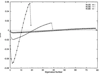
Q = diag (q(xi),q(x2),...,q(xN)) . (2.9) The advantage of this discretisation is that the resulting matrix is tridiagonal, and hence its eigenvalues are easily computed. As discussed above, the central finite differences discretisation fails to implicitly approximate the high order eigenfunc tions adequately. Thus, the high order algebraic eigenvalues do not approximate the corresponding differential eigenvalues. In the case of the central finite differ ences discretisation, it is known [8, p. 9] that for any C 2[0 ,7r] potential q(x)
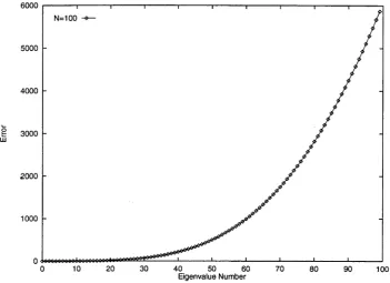
Thus, the algebraic eigenvalues are clearly non-uniform approximations to the differential eigenvalues. As an example of this, consider the null-potential system. The differential and algebraic eigenvalues of this system are known in closed form. The difference between the eigenvalues is given by
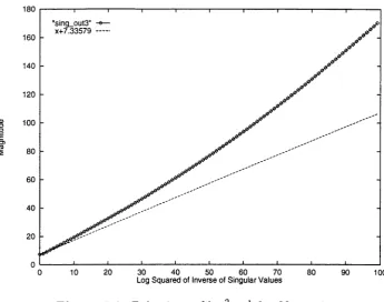
and is plotted in Figure 2.1 Clearly, for fixed A, the error in the eigenvalue approximations increases rapidly.
The algebraic correction overcomes this difficulty by adding a correction to the algebraic eigenvalues, which reduces the error (2.10). This concept of improving the numerical solution of a problem by approximating the error, and then adding it to the solution, is a classic approach used in numerical analysis. For example, extrapolation [50, 58], and multigrid [20], are based on this concept.
The key observation made by Paine et al. [70] was that the difference |Afc — /ik\ is insensitive to moderate changes in the potential q(x). Thus, if a difference of this form can be calculated for a “near-by” potential, it will approximate the error between the algebraic and differential eigenvalues for the given potential.
The natural “near-by” problem to use is the null-potential system, which is given by
\ \ k - ß k \ = 0 ( k i h2). (2.10)
Ufc(x) = X0<kUk(x) , € (0,7r),
6000
N=100
0 <9000000000^00000 0 08
Eigenvalue Number
Figure 2.1. The error between the exact and algebraic eigenvalues for the null- potential system.
The central finite differences discretisation of this problem gives - ^ A u k = A*o,JbUjfc.
As mentioned above, the eigenvalues Ao,* and //0,k are known in closed form. Thus, the difference
£ k = A0)fc — //o.jfe
may be formed, and can be used to approximate A* — //*. Paine et al. [70] proved the following theorem.
Theorem 2.1 (Paine et al. [70]) If q G C2(0 ,7r), then there exists an a < 1, independent of N , such that
Xk- Pk=£k + 0(kh2 ) ,
for 1 < k < aN .
This theorem shows that the difference Ek is an excellent approximation to the error between the differential and algebraic eigenvalues for any C 2(0,7t) potential. This result leads naturally to the definition of the approximate differential eigenvalues,
[image:25.550.97.449.109.364.2]for 1 < k < a N, a < 1. Thus
|A* - At I = 0 ( k h2) ,
which is an improvement on the error (2.10) for the uncorrected algebraic eigen values.
The difference s k will be called the algebraic correction, since it is an algebraic method of improving the eigenvalue estimates. In a sense, ek modifies the asymp totic form of the algebraic eigenvalues, bringing it closer to the asymptotic form of the differential eigenvalues. For this reason, the correction s k is known elsewhere in the literature [4, 5, 7, 9, 10, 11] as the asymptotic correction.
2 .4 E x te n s io n s to t h e A lg e b r a ic C o r r e c t i o n M e t h o d
The paper by Paine et al. [70] sparked a vigorous investigation of the algebraic correction methodology. In particular, Andrew and Paine [10, 11], and Andrew [5, 7] have made significant contributions to this field.
The extensions to the algebraic correction methodology fall into two basic classes: more general boundary conditions, and different discretisation schemes.
The first of these generalisations was examined by Anderssen and de Hoog [3]. They considered the Sturm-Liouville problem in potential form, with the more general boundary conditions
Anderssen and de Hoog [3] considered the central finite differences discretisa tion of this problem. Because the boundary conditions are more general, they introduced the augmented grid
The central finite differences discretisation of (2.12) over the uniform grid G* gives the corresponding matrix eigenvalue problem
u'k(x) + q( x) uk(x) = A kuk( x) , x G (0, n ), ai*4(0) - o 2Wfc(0) = 0 ,
Piu'kW ~ ßiUkin) = 0.
(2.12)
G* = {xj : Xj = j h , j = —1 ,0 ,1 ,..., N, N + 1, h = n / N } .
(—L + Q)vfc = crfcVfc ,
- 2 p
1 - 2 1
1 - 2 1
q - 2
where p = 2ot\/(oi\ + ha2) and q = 2ß\/{ß\ + hß2).
Anderssen and de Hoog [3] used the null-potential system - u k(x) = A0,ku{x), x
e
(0, tt) ,04*4(0) - o 2ufc(0) = 0 , ßiuk(ir) - ß2uk{ir) = 0,
as the near-by problem. The central finite differences discretisation of this gives the corresponding matrix problem
—L vfc = (JofcVfc .
In this case, because of the more general boundary conditions, A0 and cr0 are not known in closed form. However, Anderssen and de Hoog provide an iterative formula for calculating these quantities. Thus, although the algebraic correction
£ k = A0,/c — cr0,jfc
is not known explicitly, it can be calculated up to a predetermined accuracy. Anderssen and de Hoog [3] prove the following theorem, which is analogous to Theorem 2.1.
Theorem 2.2 (Anderssen and de Hoog [3]) If q
e
C 2(0,7r) then there exists an a < 1, which is independent of N, such thatA k — &k = £k + 0 ( h2) for 1 < k < aN.
This result is an improvement over Theorem 2.1, since k has been removed from the order of convergence. Andrew [4] notes that in the proof of this result, Anderssen and de Hoog assume that qx^ 0, so this result does not generalise directly to the system (2.1). Although it has not yet been done, the method of Anderssen and de Hoog [3] could probably be used to improve the result of Theorem 2.1.
Using the central finite differences discretisation, Andrew [7] extended the al gebraic correction to the case of periodic and semi-periodic boundary conditions. In particular, he considered the boundary conditions
uk{0) = uk(7r), d ( o ) = » 4 M . and
Uk{0) = - u k(ir) ,
A ndrew [7] showed th a t theorems analogous to the ones above hold in each of these cases. A ndrew ’s results are slightly stronger th an those proved in Theorem 2.1, since they are not restricted to hold only for 1 < k < a N . An exam ple of this type of result is given below.
T he next im p o rtan t generalisation to the algebraic correction m ethod was made by A ndrew and Paine [10]. They considered the problem (2.1). However, instead of the sta n d a rd central finite differences discretisation, they considered the Numerov m ethod for the discretisation of the problem.
T he Num erov m ethod approxim ates the problem (2.1) by the m atrix problem (—A + B Q )vjt = CfcBv*. ,
where
h2
B — I/v T — A . 12
Here, I,v is the N x N identity m atrix, and A and h are given as before. The advantage of the Numerov m ethod is th a t the low order algebraic eigenvalues are more accurate approxim ations to the corresponding differential eigenvalues. However, as in the central finite differences case, the approxim ation breaks down as the eigenvalue order increases. Specifically, Andrew and Paine [10] showed th a t for any C 4[0,7r] potential
= 0 ( k 6h*).
As above, Andrew and Paine [10] used the null-potential system to dehne the algebraic correction. In this case, the Numerov discretisation of the null-potential system (2.11) gives the m atrix problem
-A v*. = Co.it B v fc . The algebraic correction
£ k = N , k — Co,A;
is known in closed form. Andrew and Paine [10] proved the following theorem . T h e o r e m 2.3 (A n d re w and P a in e [10]) I f q 6 C 4(0 , 7r), then there exists a constant Cq, depending only on q, such that fo r all N G N and k = 1, . . . , N
k*h5 k C/c ^ C o —7 , , •
sin kh
The next important generalisation was again made by Andrew and Paine [11]. They examined the problem (2.1), this time imposing a finite element discretisa tion.
Andrew and Paine [11] used the “linear hat” co-ordinate functions j 1 — \x— Xj\/h if \x — Xj\ < h,
J ^ | o if \x — Xj I > h,
on the uniform grid G, in the definition of their finite element method. This leads to the corresponding matrix problem
(—A + F)v k = DkB v k . where
h2 B = Iw + — A ,
6 and
1 f n
Fij = - / q[x)4>i{x)(t)j {x) dx . h J o
Again, the algebraic eigenvalues of the finite element discretisation of (2.1) are not uniform approximations to the corresponding differential eigenvalues. Andrew and Paine [11] showed that for any C2[0,7r] potential
|Afc — i9fc| = 0 ( k 4h2) .
Andrew and Paine [11] defined the algebraic correction as the difference between the differential and algebraic eigenvalues for the null-potential system
£k = Ao,fc — $0,jfc •
Again, the algebraic correction is known in closed form. Andrew and Paine [11] proved an analogue of Theorem 2.3 for the finite element case.
T h e o re m 2.4 (A ndrew an d P ain e [11]) If q G C 2(0,7r), then there exists a constant Co, depending only on q, such that for all N E N and k = 1, . . . , N
k2h3
Afc - Vk\ < Co——— .
sm kh
Andrew [5] extends the above result to more general boundary conditions. In particular, he proves analogous theorems for the natural boundary conditions
*4(0) = 0 = *4(7r),
Uk{0) = 0 = u'k(n),
and the periodic and semi-periodic boundary conditions M 0) = uk(ir) ,
“ 1(0) = u'k(ir) , and
Ufc(0) = ,
“ 1(0) = -u l(jr) ■
Notice that, as in the case of Theorem 2.1, the results of Theorems 2.2-2.4 lead naturally to the definition of approximate differential eigenvalues, which are better approximations to the exact differential eigenvalues than the uncorrected algebraic eigenvalues.
One further extension to the algebraic correction will be considered. This ex tension is motivated by considering the use of the algebraic correction in solving the inverse eigenvalue problem for (2.1). Since the extension is intimately connected with difficulties associated with solving the inverse problem, it will be defined in Chapter 3.
2 .5 N u m e r ic a l R e s u lts
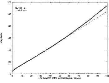
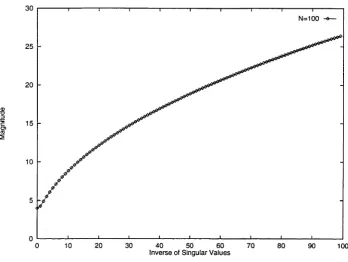
Significant numerical studies have been carried out on the algebraic correction, for the original method [70], and each of the extensions [3, 10, 11]. In this section, the numerical performance of the original algebraic correction will be considered. Some characteristics of the algorithm will be considered, which will be of importance in the next chapter.
For the problem (2.1) under the central finite differences discretisation, the algebraic correction is known in closed form, and is given by
4 . 2 kh
Thus, the approximate differential eigenvalues are given by
For the potential
q(x) = 6 cos 2x , (2.13)
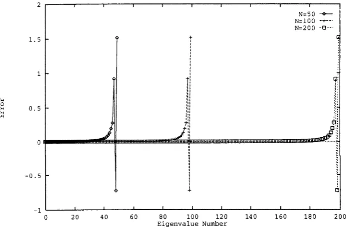
shooting method, to calculate the eigenvalues of a regular Sturm-Liouville prob lem. The numerical tolerance was set to 10“7, and the resulting eigenvalues were used to determine the error in the approximate differential eigenvalues calculated by the algebraic correction. The NAG routine F02AAF was used to calculate the algebraic eigenvalues of (2.7) for the potential (2.13). The approximate differential eigenvalues were then calculated, and the error
error = \ k - \ k (2.14)
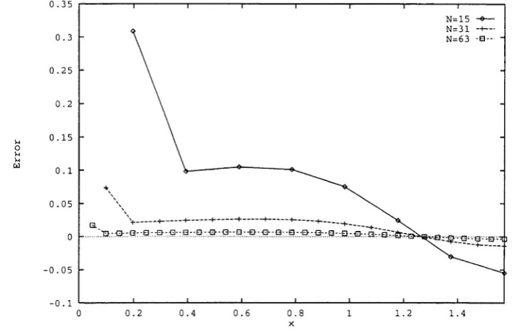
determined. This error is shown in Figure 2.2, for N = 50, 100 and 200.
N=50 -o— N=100 -+— N=200
-0.5
80 100 120 Eigenvalue Number
F ig u re 2.2. The error (2.14) for the potential (2.13).
The algebraic correction has given an excellent approximation to the differential eigenvalues in its range of applicability. For example, compare Figure 2.2 with the uncorrected approximation in Figure 2.1. Recall that the proof of Theorem 2.1 shows that the algebraic correction holds only for 1 < k < aN. Outside this range, the approximation breaks down. Notice that Figure 2.2 shows that an error
bound of the form „ „
k2h3 C°sin kh ’ proved by Andrew [8] is sharp.
[image:31.550.99.452.276.508.2]eigenvalues calculated by the algebraic correction converge pointwise to the cor responding differential eigenvalues; i.e., any fixed eigenvalue approximation will converge to the corresponding exact eigenvalue, when N becomes large enough. However, due to the non uniform structure of the error, the approximate eigenval ues do not converge uniformly to the exact eigenvalues. This observation will be important in the next chapter, when the difficulties encountered in applying the algebraic correction to the solution of the inverse problem are considered.
T h e O n e -D im e n s io n a l In v e rs e E ig e n v a lu e
P r o b le m
3 .1 I n tr o d u c tio n
The one-dimensional inverse eigenvalue problem is more difficult to solve than the corresponding forward problem. Determining solutions of the inverse formulation is less intuitive, and the improperly posedness of the problem makes reconstruc tion algorithms unstable. A numerical method for reconstructing the potential in the inverse formulation of the Sturm-Liouville problem suffers from several diffi culties. Firstly, only a finite amount of data can be used in the reconstruction, and so uniqueness of the resulting potential cannot be guaranteed. Algorithms for reconstructing the finite dimensional problem from the given data also tend to be unstable. Thus, any error in the given data can dramatically affect the re construction process. Finally, some care must be taken to ensure that the given data for the continuous problem is consistent with the data required for the finite dimensional problem.
To overcome the difficulty of loss of uniqueness, additional constraints may be placed on the potential. These often take the form of assuming that the given problem is “near-by” to some reference problem. The improperly posed ness of the inverse formulation is a fundamental difficulty. However, with some care, stable algorithms for reconstructing the finite dimensional problem can be formulated [27, 37]. In certain circumstances, regularisation techniques may be applicable to reduce the affect of the improperly posedness of the reconstruction algorithm. This has been successfully applied by Paine [67]. The difficulty with regularisation techniques is that they can adversely affect the numerical solution, if they are not implemented carefully.
In this section, the question of consistency of the finite dimensional problem is considered in detail. A method due to Hald [40], based on the Rayleigh-Ritz dis cretisation is discussed, and is shown to be consistent. Unfortunately, the algorithm involves the reconstruction of a dense matrix, which can be quite slow computa tionally. From Chapter 2, it follows that a reconstruction method based on the
central finite differences discretisation will not be consistent, since the differential eigenvalues are not well approximated by the corresponding algebraic eigenvalues. Paine [68] was the first to consider using the algebraic correction methodology, in reverse, to overcome this difficulty. The main focus of this Chapter is on analysing Paine’s method, and developing a modification to the original algorithm which gives improved convergence.
Before discussing the consistency of numerical algorithms for solving the inverse problem, an intuitive explanation of the improperly posedness of the problem is presented. Consider the one-dimensional Sturm-Liouville problem with Dirichlet boundary conditions
There are three conditions which a problem must satisfy in order to be properly posed [49]. They are:
1. Existence of a solution under the given conditions. 2. Uniqueness of the solution under the same conditions. 3. Continuous dependence of the solution on the given data.
The first two points have been dealt with by Gel'fand and Levitan [33], and Borg [17] respectively. Recall that Borg [17] showed that further information is required to guarantee a unique solution to this problem. This fact is itself an indication of the improperly posedness of the problem.
Recall from Chapter 1 that (3.1) has a countably infinite number of eigenvalues. Suppose the potential q(x) is continuous. Then the potential may be uniquely characterised by determining a countably infinite set of points q ( x , on the graph of the potential. Thus, in the formulation of the inverse problem for (3.1), there is a countably infinite amount of data (the eigenvalues Ak) and a countably infinite number of unknowns (the points on the graph of the potential q(x) which determine it uniquely). Thus, intuitively, one would expect that the inverse problem in this form would be well posed. To see that this data is not enough, consider the problem (3.1) in Rayleigh quotient form
Recall that the leading term in the asymptotic expansion of uk(x) is sin kx. Sub stituting this into the above equation and removing constant terms gives
uk(x) + q{x)uk(x) = Akuk(x) , x € (0, tt) uk(0) = 0 = uk(t t) .
(3.1)
foW'k{x)]2dx + fp q(x)[uk(x)]2dx

![[N709.Ebook] Ebook Download Blood Noir Anita Blake Vampire Hunter Book 16 By Laurell K Hamilton.pdf](data:image/gif;base64,R0lGODlhAQABAIAAAP///wAAACH5BAEAAAAALAAAAAABAAEAAAICRAEAOw==)