Reproductive change in Ghana : evidence from two national surveys

REPRODUCTIVE CHANGE IN GHANA : EVIDENCE FROM TWO

NATIONAL SURVEYS

^

U N l V t ^ '

By

BENJAMIN E. AMENUVEGBE

A thesis submitted for the degree of

Doctor of Philosophy

of the Australian National University

DECLARATION

Except where it is indicated otherwise, this thesis

ACKNOWLEDGEMENTS

I would like to express my gratitude to the Australian National University for awarding

me the scholarship which made this research possible. I greatly appreciate the generous

facilities for research that I had at my disposal in writing this thesis.

I also wish to express my deep appreciation to my supervisor, Professor Gavin W. Jones

for his guidance, encouragement and support in writing this thesis. Prof. Jones promptly

read my drafts and suggested very useful improvements at various stages of this study.

He often invited me for discussions and generously gave me any reading materials from

his own library which are relevant to our discussions for my use. I am very grateful for

his kindness.

I am also very grateful to Dr Allan Gray for willingly reading the entire thesis and

making very useful comments on the statistical procedures used in the analysis. He also

willingly spent time discussing several methodological problems that I brought to his

attention on a number of occasions. My special thanks also go to Prof. Ian Diamond

who had several discussions with me at the beginning of this thesis. I thank Drs S.

Phillip Morgan, Phillip Guest, Habte Tesfaghiorghis, Gordon Carmichael, Gigi Santow

and Prof. Jack Caldwell all of whom at one time or the other made useful suggestions to

me about some aspect of this thesis. I have also benefited a great deal from numerous

discussions I had with my friend Tetteh Dugbaza about various aspects of human

reproduction in Ghana and I am very grateful for his willingness to share his knowledge

with me at various times.

I highly appreciate the help of Ms Yvonne Pittlekow of the Computing Section in the

Research School of Social Sciences and Ms Jill Jones formerly of the Demography

Program in solving several data management and programming problems in the course of

writing this thesis. I also thank Mr Gavin Longmuir for his help in solving a number

computer related problems and Pat Quiggin for her help in locating relevant reference

material on may occasions.

My thanks also go to Mrs Wendy Cosford for her help in editing the thesis. Her editorial

advice is very much appreciated. I also thank Ms Lydia Mensah for her help in typing

parts of this thesis. I am grateful to all other members of staff for the friendly

ABSTRACT

This analysis examines various aspects of human reproductive change based on the

Ghana Fertility Survey (GFS) and the Ghana Demographic and Health Survey (GDHS).

It compares the data on transition to parenthood, birth spacing and durations of

breastfeeding, postpartum amenorrhoea and abstinence and the factors influencing

them. The study also dealt with the use of modem contraception as well as the

relationship between the survival status of a child and the time to the next birth. The

consistency in the measurement of selected variables in both surveys was also

examined.

There was considerable agreement in the measurement of birth intervals and the effects

of factors affecting them. Consistency has been demonstrated in the measurement of the

second, fifth and sixth birth intervals and also in the effect of selected independent

variables examined in the two surveys. Age at first marriage, first birth and the first

birth interval do not appear to be comparable in the two surveys; this is also the case

with the third and the fourth birth intervals. This finding is not surprising because of

problems of measurement of marriage data in Africa which result from the fact that it is

often a process rather than an event at a point in time.

The finding of inconsistency of measurement of age at marriage and the first birth

interval implies that these data may not be pooled from the GFS and the GDHS to obtain

a larger and possibly more stable series; also it is necessary to exercise caution in

interpreting observed differences when such data are compared for the GFS and GDHS.

On the other hand the consistency found shows reliability of the data though at aggregate

level, and thus considerably increases our confidence in the comparative results.

The study found general stability in the pace and quantum of fertility. The overall

distribution of the second birth interval is only marginally different for the two surveys;

The distribution of the second to the fourth intervals are fairly symmetrical though the

younger cohorts appear to show slightly longer delays for these births.

Age at first marriage and age at first birth also appear to be generally stable within and

between surveys though small increases are observed for later periods and younger

cohorts. The only significant differential for age at first birth is education: women with

11 or more years had higher ages at first birth in both surveys.

Median durations of breastfeeding and postpartum sexual abstinence either are stable or

have increased slightly between the GFS and GDHS. A positive relationship is found

between birth interval length and breastfeeding duration and also between fertility on the

one hand and amenorrhoea and abstinence on the other indicating the importance of

these postpartum factors for fertility. Median durations of postpartum amenorrhoea are

found to generally exceed those of postpartum sexual abstinence. This suggests that

amenorrhoea is more important for birth spacing than sexual abstinence among the

respondents.

Since failure time data from large-scale surveys are usually heavily tied, the grouped

proportional hazard model is applied to determine important factors influencing age at

first birth, birth intervals as well as breastfeeding and postpartum amenorrhoea and

abstinence. Ethnicity, place of residence and education are found to be significantly

related to breastfeeding and postpartum sexual abstinence in both surveys.

Finally, the analysis showed a positive relationship between breastfeeding and birth

interval length which indicates the contraceptive effect of breastfeeding, and implies that

the long periods of breastfeeding in Ghana are advantageous not only for the sake of

infants' health but also for birth spacing. Since effective contraceptive use is low, and the

women tend to bear children throughout the reproductive life-span, long breastfeeding

This analysis concludes that there is only a weak evidence for reproductive change. Few

and generally weak differentials were observed within and across surveys. Also, lack of

significant association between postpartum variables and age and parity indicates stability

of fertility decline. Except for the weak evidence mainly associated with recent periods

and also younger cohorts, the pace and quantity of fertility appear to be stable.

TABLE OF CONTENTS

DECLARATION...ii

ACKNOWLEDGEMENTS... iii

ABSTRACT...v

TABLE OF CONTENTS...viii

LIST OF TABLES... xiii

LIST OF FIGURES...xvi

CHAPTER 1

INTRODUCTION...1

1.1 Birth interval and fertility dynamics... 2

1.2 Some problems of human reproductive research in Africa... 3

1.3 Advantages of multiple surveys for measuring reproductive

change... 5

1.4 Overview of some recent findings about reproduction in

Ghana... 6

1 .4. 1 Differentials in trends...7

1.4.2 Age at marriage... 8

1.4.3 Contraception... 9

1.4.4 Breastfeeding... 9

1.4.5 Infant and child mortality...10

1.5 Objectives of the study... 10

1. 6 Rationale for the study...11

1.7 Outline of main analytical procedures...12

1.7.1 Notation... 12

1.7.2 Life table methods... 13

1.7.3 Life-tables and regression...15

1.7.3.1 The proportional hazards model...16

1.7.3.3 Grouped data proportional hazards model... 17

1.7.3.4 Derivation of the likelihood function for

grouped data...18

1.8

Outline for the thesis...19

CHAPTER 2

EXPLANATIONS OF FERTILITY DECLINE : AN

OVERVIEW...20

2.1 Introduction...20

2.2 Theories of fertility decline... 20

2.2.1 The classical fertility transition theory... 20

2.2.2 The Threshold Hypothesis... 22

2.2.3 Micro-economic theories of fertility decline...22

2.2.5 Ideational theories... 25

2.2.6 Intergenerational wealth flow th e o ry ... 26

2.2.7 Institutional facto rs...27

2.2.8 Proximate D eterm inants...28

2.3 Infant and child mortality and fertility d eclin e... 29

2.3.1 Actual infant and child mortality and fertility decline... 31

2.3.2 Perceived mortality and fertility decline...32

2.3.3 Family planning, child mortality and fertility decline... 32

2.4 Conclusion... 33

CHAPTER 3 THE SAMPLES AND THE CH A R A C TERISTICS...37

OF RESPONDENTS 3.1 Introduction...37

3.2 The surveys... 37

3.2.1 The G FS...37

3.2.2 The G D H S ... 38

3.3 Background variables... 39

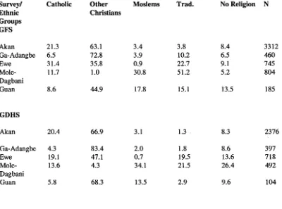
3.3.1 Ethnicity...39

3.3.2 Religion...40

3.3.3 Education... 42

3.3.4 Place of residence...43

3.3.5 Type of w ork...44

3.4 Association between background variables...45

3.4.1 Ethnicity and religion... 47

3.4.2 Ethnicity and residence...48

3.4.3 Region and ethnicity... 49

3.4.4 Age, current residence, religion and education...50

3.4.5 Ethnicity and education...52

3.5 Measures of the strength of association among background variables... 53

3.5.1 Nominal and ordinal variables... 54

3.6 Conclusion... 57

CHAPTER 4 ASPECTS OF DATA Q U A LIT Y ... 59

4.1 Introduction...59

4.2 Sampling and non-sampling e rro r...59

4.2.1 Quality of age data...60

4 .3 Quality of birth reporting... 64

4.3.1 Omission of births...65

4.4 Quality of data on exposure to the risk of childbearing... 66

4.5 Problems of differential data quality... 67

4.6 Comparability of data in the GFS and the GDHS surveys...

65

4.6.1 Limitations of CSS for measuring change...69

4.6.2 Advantages of successive fertility surveys... 71

4.7 Data and m eth o d s...75

4.7.1 The d a ta ...75

4.7.2 The m eth o d ... 75

4.7.3 Statistical test procedures... 7§

4.8 Results...1%

4.8.1 Shifts in mean levels... 7%

4.8.2 Consistency in covariate effects... 4.9 Conclusion... ^1

CHAPTER 5 A COMPARATIVE ANALYSIS OF AGE AT FIRST MARRIAGE AND FIRST B IR TH ... 82

5.1 Introduction... 82

5.2 Socio-economic and biological context of transition to parenthood...82

5.2.1 Economic considerations...84

5.2.2 Biological constraints...8S 5.3 The relationship between premarital births and m arriage... 8<5 5.4 The start of family formation in G h an a... 85

5.5 Data and m eth o d s...87

5.5.1 Dependent variables...87

5.5.2 Independent variables...88

5.5.3 Some measurement problem s...9 0 5.5.4 Comparability of data... 9 0 5.6 Method of A nalysis...92

5.7 Results and Analysis...9 4 5.7.1 Age at first m arriage...9 4 5.7.2 Age at first b irth ... 97

5.7.3 Life table analysis of the first birth interval...99

5.7.4 Age, cohort and period effects... 99

5.7.4.1 Age effects... 1 Ol 5.7.4.2 Cohort e ffe c ts... 102

5.7.4.3 Period effect... IO4. 5.8 Multivariate analysis...10S 5.8.1 Socio-cultural determinants of age at first b irth ...105

5.8.2 Multivariate analysis of the age at first b irth ...105

5.9 Conclusion... 107

CHAPTER 6 A COMPARATIVE ANALYSIS OF INTER BIRTH IN TERV ALS... 109

6.1 Introduction... 109

6.4 Some problems of birth-interval analysis...

114-6.5 Data and data managem ent... 115

6.5.1 Comparison of questions on covariates... 116

6.5.2 Dependent and independent variables...116

6.5.2.1. The dependent variable...116

6.5.2.2 Choice of birth intervals... 117

6.5.2.3 Independent variables... 118

6.6 M ethodology... 119

6.6.1 Life table m ethods...119

6.7 Multivariate Analysis... 120

6.8 Analysis and results...121

6.8.1 Comparison of mean length of intervals... 12 \

6.8.2 Comparisons for comparable cohorts...122.

6.9 Time series analysis...12 S 6.9.1 Five years before either survey... 12& 6.9.2 Ten years preceding survey... 129

6.9.3 Twenty years before su rv ey ... 129

6.10 Life table analysis... 130

6.11 Multivariate analysis...13*1 6.12 Conclusion... 140

CHAPTER 7 OTHER FACTORS AFFECTING LENGTH OF BIRTH INTERVALS...14!

7.1 Introduction...14!

7.2 Some previous related research... 143

7.2.1 Breastfeeding... 143

7.2.2 Postpartum sexual abstinence...14 5 7.2.3 Infant and child mortality and subsequent fertility...146

7.3 Data problems and m anagem ent... 14 7 7.3.1 Reported durations of breastfeeding, amenorrhoea and abstinence... 149

7.3.2 Current-status breastfeeding d a ta ...154

7.3.3 Selection effects... 155

7.3.4 Measurement of postpartum variables...155

7.3.5 Other problems associated with breastfeeding data... 156

7.3.6 Sample and variable selection...157

7.3.7 Choice of explanatory variables... 15& 7.4 Data analysis and methods... 16D 7.4.1 Cox's proportional hazards m o d el...160

7.4.2 A ssum ptions... 161

7.4.3 Model selection... 162

7.5 Results and discussion... 163

7.5.1 Durations of breastfeeding, amenorrhoea and postpartum sexual abstinence in the open and last closed intervals... 163

7.5.2 Correlations among postpartum variables parity and age at ev en t...164

7.5.3 Further examination of the relationship between

postpartum variables and fertility... .1 6 6 7.5.4 Proportional hazard analysis...17 0 7.5.5 The use of modem contraception... .1 7 3

7.5.5.1 Basic formulation of the logistic m odel... .174« 1.5 .5 2 Model selection... .175

7.5.5.3 Interpretation of estimates of model

param eters... 175 7.5.5.4 Current use of modem contraception... 176 7.5.5.5 Ever use of modem contraception...179 7.5.6 Infant and child mortality and fertility... l&l 7.6 Conclusion...

184-CHAPTER 8... 185

LIST OF TABLES

Table 3.1 Percentage distribution by background variable by survey... 41

Table 3.2 Percentage distribution of respondents by ethnicity, religion

and survey...48

Table3.3 Percentage distribution of respondents by ethnicity, type of

place of residence by survey... 49

Table 3.4 Percentage distribution of respondents by region of residence

by ethnicity by survey... 50

Table 3.5 Education by age, type of residence and religion...51

Table 3. 6 Age by ethnicity, education and by survey... 53

Table 3.7 Lambda and gamma measures of associations between pairs of independent variables by survey... 56

Table 4.1 Showing comparison of selected fertility indicators by survey... 7S

Table 4.2 F-statistics for Study effects for predictor variable for the

selected fertility indicators...SO

Table 5.1 Distribution of form of responses for age at first marriage and

first birth by survey...

92-Table 5.2 Mean Age at First Marriage by Selected Covariates by Survey...9 6

Table 5.3 Median Age at First birth by Selected Covariates by Survey... 9&

Table 5.4 Unstandardised quartiles of the distribution of the first birth

interval by survey... 100

Table 5.5 First birth interval by age at start of interval by survey...| Q|

Table 5.6 Summary measures of the life table analysis of the first birth

interval by age cohort and by survey...10^

Table 5.7 Summary measures of the life-table analysis of the first birth

interval by calender period and by survey...104

Table 5.8 Exponentals of Discrete Time Proportional Hazard Co­

efficients for Age at First Birth by S urvey...106

Table 6.1.1 Mean second birth intervals by comparable age cohort by

survey...123

Table 6.1.2 Mean third birth intervals by comparable age cohort by

survey... 123

Table 6.1.3 Mean fourth birth intervals by comparable age cohort by

survey... 124

Table 6.1.4 Mean fifth birth interval by same age cohort by survey...124

Table 6.1.5 Mean sixth birth interval by comparable age cohorts by

survey... 125

Table 6.2.1 F-statistics for differences for yearly change in average

interval length for all intervals by survey...128

Table 6.2.2 F- statistics for the significance of linearity for data in Table

6

.2.1...

Table 6.3.1 Selected life table measures for birth intervals two to four

by Survey... 131

Table 6.3.2 Summary life table statistics for birth intervals two to four

for age cohorts by survey...

132-Table 6.3.3 The quantum and the trimean by cohort and by survey...IBB

Table 6.3.4 Showing values of the D statistics for the distributions of the

Table 6.4.3

Estimated regression co-efficient from discrete time Cox

proportional hazard model:...13g,

Table

7.5.1 Medians of the distribution of breastfeeding, amenorrhoea

and sexual abstinence in the open and closed intervals by ethnic group and

by survey... 163

Table

7.5.2 Estimates of coefficients of correlation between durations of

breastfeeding amenorrhoea abstinence and parity and age of mother at

birth for the last closed interval by ethnicity by survey... 165

Table 7.5.3

Medians of the distribution of amenorrhoea and abstinence

in the open interval by breastfeeding status...167

Table 7.5.4

Breastfeeding duration and the length of the last closed birth

interval... 16$

Table 7.5.5

Average duration of the last closed birth interval for varying

lengths of amenorrhoea... 16^

Table 7.5.6

Median duration of the last closed birth interval for varying

lengths of abstinence... 1*70

Table

7.5.7 Exponentials of proportional hazards co-efficients (RR) of

the breastfeeding duration in the open birth interval... 1*71

Table

7.5.8 Exponentials of proportional hazards co-efficients (RR) of

the sexual abstinence duration in the open birth interval... 172

Table 7.5.9

Logistic regression model estimates for the effects of

selected background variables on the current use of modem

contraception... 177

Table 7.5.10

Probabilities of current use of modem contraception for

selected covariate patterns by survey... 17&

Table 7.5.11

Logistic regression model estimates for the effects of

selected background variables on the everuse of modem contraception... 1$0

Table 7.5.12

Average length(months) of the second to the sixth birth

intervals by survival status of the child initiating the interval...182,

Table 7.5.13

Average length of the last closed interval by survival status

LIST OF FIGURES

Figure 6.2.1

Time series graph of mean birth intervals for the GFS and DHS...

127

Figure 6.3.1

Graph of the cumulative hazard functions for the second birth

interval... 134

Figure 6.3.2

Graph of the cumulative hazard functions for the third birth

interval... 134

Figure

6.3.3 Graph of the cumulative hazard functions for the fourth birth

interval... 13S

Figure 7.3.1

Per cent distribution of reported durations of breastfeeding in the last

closed interval for the GFS and GDHS

data...151

Figure 7.3.2

Per cent distribution of reported durations of postpartum amenorrhoea in

the last closed interval for the GFS and

GDHSdata... 151

Figure 7.3.3

Per cent distribution of reported durations of postpartum sexual abstinence

in the last closed interval for the GFS and

GDHS...

151-Figure

7.3.4 Per cent distribution of reported durations of breastfeeding in the open

interval for the GFS and GDHS

data...151

Figure

7.3.5 Per cent distribution of reported durations of postpartum amenorrhoea in

the open interval for the GFS and GDHS

data...15

,

Figure 7.3.6

Per cent distribution of reported durations of postpartum sexual abstinence

in the open interval for the GFS and GDHS

CHAPTER 1

INTRODUCTION

This study compares several aspects of reproductive change in the Ghana Fertility

Survey (GFS) conducted in 1979 and the Ghana Demographic and Health Survey

(GDHS) conducted in 1988, which were both representative samples of the population

of Ghana. In particular, it deals with family formation, birth spacing and related socio­

cultural factors and emphasizes the advantages and disadvantages of using multiple

surveys for measuring such change. The main approach adopted is to compare transition

times to specified fertility events as well as the effects of selected background variables

in the two data sets. With the additional data provided in the GDHS, it is possible to

examine elapsed time for making specific transitions as well as trends in effects of the

background variables. Specifically, the study seeks to determine whether on average the

pace of closing specific birth intervals is increasing, decreasing or uniform and whether

the effect of the selected background variables on the transition times as well as some

other reproductive events is the same or different for the two surveys.

The analysis discusses the quality of age data, birth reporting, and data on exposure to

the risk of childbearing and compares the consistency of measuring aspects of average

reproductive experience for the same birth cohorts of women who are in both surveys.

Besides comparing the consistency of time to occurrence of selected reproductive

events, the consistency of the measurement of the effects of independent variables for

birth interval distributions are also examined. Key dependent variables in the study are

birth interval distributions, age at first marriage and first birth and use of modem

contraception, which are analysed for selected groups in the population. Breastfeeding

with post partum sexual abstinence and with use of modem contraception are examined,

residence, which have been variously shown to be related to fertility in many

demographic studies.

An important aspect of the study is the estimation of the quantum and tempo of fertility

for categories of selected covariates. Two aspects of birth intervals are studied: the first,

to obtain and compare selected summary indices for distributions of completed and

incomplete intervals using life-table techniques; and the second, to use hazard modelling

to study the factors associated with lengths of intervals. Also, time series analysis is used

to compare changes in the average length of birth intervals over time. This procedure

involves pooling all intervals individually for the surveys, together with the year the

interval was closed, and using statistical tests to determine if there were significant

variations in average interval length by year of closure by survey and by selected

durations

1.1 Birth interval and fertility dynamics

The role of birth intervals in the causal chain of factors which determine the birth rate has

been described by Bogue and Bogue (1980). According to this explanation, socio­

cultural, economic and psychological factors influence the methods, duration and

regularity of contraception, which in turn influence the conception time to live births and

the open birth interval. Also the exposure to pregnancy, influenced by these socio­

cultural, economic and psychological factors, in turn affects birth intervals. A third

factor, fecundability, influences both the practice of contraception and birth intervals.

The length of the closed and open birth intervals determines the birth rate.

Fecundability is the probability that a conception will occur in a given month. Variation

in fecundability consists of variation from one woman to another as well as variation

over time for a particular woman and is the result of several factors which interact with

successful pregnancy: normal ovulation during a menstrual cycle, timing of sexual

intercourse, sperm count and absence of structural or other obstacles that could prevent

the union of sperm and ovum, the capacity of the uterus to retain and nourish the

fertilized ovum and the viability of the growing foetus. The authors contended that these

factors are difficult to quantify separately since they are numerous and are subject to

individual variation. On the other hand the socio-cultural and economic factors which

influence reproductive behaviour are relatively more measurable in surveys and can

contribute to differences in observed time that elapses between marriage and conception

and also between successive high-order births. The present study deals only with these

latter factors.

1.2 Some problems of human reproductive research in Africa

There is an increasing need to know and monitor the changing pattern of the birth rate

and other reproductive behaviour, particularly in sub-Saharan Africa. This region shows

the least sign of fertility decline although there is now a notable downward trend in

South Africa, and recently in Zimbabwe, Botswana, and Kenya (see McNicoll, 1992)

This has important implications because of the increasing consensus that the control of

population growth is a prerequisite for freeing resources for economic development. For

example, participants at a recent African Development Bank conference pointed to rapid

population growth as one of the main obstacles to Africa's development and

recommended, among other things, research into related attitude and behaviour changes

in Africa (see West Africa, October, 18-24, 1993).

Problems of effective research in understanding attitude and behaviour changes that

affect reproduction in Africa include the scope of the research and the nature of the data

required. Specific issues that arise concern the accuracy as well as adequacy of the data.

Both problems arise because of the nature of the data collection system: for example,

errors in the data are often due to the fact that the data are obtained retrospectively by

means of memory recall. Also, large-scale surveys by their nature are usually not able to

obtain the depth of information required to understand fertility dynamics. Caldwell

(1985) argued that among other things, all large-scale surveys have three problems:

insufficient density of questions, difficult questions asked too quickly and forced

answers. These problems often arise because of the difficulty of balancing the goals of

economy, efficiency and accuracy in survey practice and there does not appear to be any

easy solution at the present time.

McNicoll (1992) pointed out that differences in socio-political organization, economic

conditions, culture and policy direction have resulted in different paths for fertility

decline in the Third World; unresolved issues include the relative import of structural and

cultural dimensions in the decision making process and what causes these to change.

This implies that an effective measurement of fertility dynamics can be greatly facilitated

if measurement instruments adequately record these relevant dimensions of human

reproduction, that is, determinants of fertility in the Third World. For example, he notes

that though there exists a great deal of demographic literature on the determinants of

fertility in the Third World, much of research fails to recognize and treat social change as

a central issue.

One aspect of this difficulty is that many social phenomena are difficult to measure

directly and often one can only contend with measuring some proxy of the phenomenon.

We have noted the criticism of the inability of large-scale surveys to measure factors that

explain fertility change. Indeed McNicoll (1992) noted that the contribution of fertility

surveys including the GFS and the GDHS to understanding of fertility is controversial, as

some feel that these surveys reveal little beside a fringe of proximate determinants; and

he argued that the emphasis on comparability of data has been detrimental to

experimentation and creativity except for technical demographic measurements. He also

argued that though these surveys did establish differentials according to a few standard

precisely than has hitherto been possible, influences on fertility at deeper levels of socio­

economic and cultural systems continue to be obscure.

Another issue is the cross-sectional nature of fertility surveys. Single cross-sectional

survey data are known to have limited potential for measuring change; one reason for

this is that these surveys take only snapshot pictures of the phenomena at one point in

time. Furthermore retrospective data which have the potential of better elucidating

change are often distorted by memory errors. When two or more demographic surveys

with retrospective reproductive data become available for the same population at

different points in time, it becomes possible to evaluate the nature of fertility change

better than can be done with one survey. This point is discussed further in the next

section. The analysis in this study uses the advantages offered by two Ghanaian national

surveys, the Ghana Fertility Survey (GFS) and the Demographic and Health Survey

(GDHS) to examine the process of recent reproductive change in the country. Finally,

the availability of the two surveys is exploited to examine the consistency in the

measurement of several reproductive events.

1.3 Advantages of multiple surveys for measuring reproductive change.

Several researchers have noted the advantages in using sufficiently comparable

sequences of cross-sectional fertility surveys to evaluate fertility change more efficiently

than is possible with a single cross-section (Hobcraft and Rodriguez, 1982; Swicegood,

Morgan and Rindfuss, 1984; Caldwell, 1985; Pullum, Casterline and Shah, 1987; Stoto,

1988). Such multiple data sources provide a good opportunity to study recent

developments in trends in reproductive behaviour and changes in trends as well as

concomitant factors that tend to influence the observed trends. This is possible because

the event history data on reproduction obtained at two different periods in time can be

used to map out change in patterns of child bearing by age, marriage duration, parity,

and intermediate variables. Furthermore the retrospective information makes available to

the analyst overlapping event histories which can be used to check the consistency with

which average fertility change is captured by the various surveys. The GFS was

conducted in 1979; the GDHS in 1988. Cohorts which were first observed in 1979 were

by 1988 nine years older, and had further experience in their reproductive careers. The

GDHS data gives the opportunity to have a second look at these and to examine the

manner and the extent to which fertility has changed. An important part of the analysis is

to determine how consistent the measurement of aspects of recent reproductive change

are in the two surveys. This is essential for comparative analysis of data from the

surveys. Further discussion of data quality and comparability is done in chapter four of

the study. In the next section, some findings about issues related to reproduction in

Ghana are provided.

1.4 Overview of some recent findings about reproduction in Ghana

Several analyses of recent fertility change in Ghana based on the GFS data have indicated

some fertility decline from about the 1970s. The GFS data (Central Bureau of Statistics,

1983) and its evaluation report (Owusu, 1984) showed that Ghana's total fertility rate

(TFR) declined by about half a child from the early 1970s. Shah and Singh (1985)

showed that the decline in the level of fertility at the national level was about 10 per cent

in the period 1960-4 to 1975-9 with most of the change (6.5 per cent) occurring in the

period 1970-4 to 1975-9. This decline in fertility was more noticeable for age group 15-

19 and for those aged 30 or above and appeared to be more rapid for higher birth orders.

This analysis suggested that lasting fertility decline may have begun in Ghana. There has

been some speculation about the nature of the possible effect of Ghana's economic

problems in the 1970s on this observed fertility decline. The period was characterized by

declines in earnings from its principal export crops, political upheavals and out-migration

of mainly young men and women to work in neighbouring countries. While the decline

in fertility that has been observed immediately before the GFS survey could be due to the

period 5-15 years before the survey resulting in an apparent rise of fertility in earlier

periods and a decline in the more recent ones, it could also be due to the out-migration in

the period (see Shah and Singh (1985). However, no categorical statements can be

made about the effect of this exodus since its magnitude is unknown.

The GDHS data however showed no conclusive evidence of a continuing decline in

fertility in the 1980s (Ghana Statistical Service, 1988). Age-specific fertility rates for

five-year periods preceding the GDHS suggest a small overall decline during the past 20

years. For women in the 15 - 19 age group fertility appears to have declined steadily at

the rate of 7 - 8 per cent in each five-year period over the last 25 years. Among women

currently in their twenties, smaller declines ranging from 1 to 5 per cent are observed for

each five year period except the period between 20 - 24 and 1 5 - 1 9 years before the

survey where fertility appears to have been stable or to have increased slightly. Women

who were in their thirties at the time of the survey showed slightly larger fertility declines

in the period between 5 - 9 and 0 - 4 years before the survey. In general, the GDHS

data showed fertility levels similar to those of the GFS. The TFR for women aged 15-44

years in the five years preceding the survey is 6.1 in the GDHS and 6.3 in the GFS.

1.4.1 Differentials in trends

In the GDHS, the TFR in the five years before the survey increased from about 3.6 for

women with more than middle school education to 6.8 for women with no education

(Ghana Statistical Service, 1988). The most significant differences are observed between

women who have higher education and all other women. Similarly, in the GFS,

substantial differences (more than two births) were observed only for women with higher

education. The decline in fertility for this survey was not always uniform as a woman's

educational level rose; several instances of curvilinear relationships were observed with

rising fertility up to primary and at times middle school level followed by a fall (see Shah

and Singh, 1985).

A similar pattern of differentials in fertility is observed for administrative regions which

coincide somewhat with ethnic residential patterns. The regions also have somewhat

different levels of development, with Greater Accra, Ashanti Central and Eastern regions

being probably the more developed than Volta, Western, Northern and Upper regions.

In the GFS differences in fertility levels for regions for the period 1975-9 have been

found to be relatively small, except that Greater Accra with 5.0 children had the lowest

average total fertility compared with 7.1 for Western or Central and 6.5-6.7 for the other

regions. Regional differentials in fertility levels in the five years before the GDHS

indicate that Greater Accra had the lowest level of fertility (TFR, 4.6), followed by

Eastern and Ashanti Regions with TFRs below 6.0, while the other regions recorded

TFRs between 6.1 and 6.9. Fertility differentials in education and ethnicity can be

influenced somewhat by differences in practices relating to age at marriage, breastfeeding

and other postpartum practices as well as differences in contraception. They may also be

influenced by individual as well as community reaction to infant and child deaths. Some

previous findings for these factors in Ghana are noted below.

1.4.2 Age at marriage

As in most Third World countries, marriage is universal in Ghana. Aryee (1985) found

that changes in age at marriage for different cohorts vary only moderately from older to

younger cohorts and that age at marriage among highly educated women (that is, 10

years and above of schooling) as well as among women with no schooling, has been

increasing from older to younger cohorts. The median age of first marriage for women

between 20 and 49 was 18 years according to both the 1979 and the 1988 surveys.

While in the GFS, 31 per cent of women aged 1 5 - 1 9 years were ever married, the

equivalent figure was about 25 per cent in the GDHS data; this suggests a slight decrease

in early marriage. Further evidence from the 1979 survey shows that while about 66 per

age-groups 72 to 77 per cent were in union before age 20. Corresponding figures for the

GDHS are 65 per cent and 73 to 77 per cent (Ghana Statistical Service, 1988).

1.4.3 Contraception

Knowledge of methods of contraception is widespread and is on the increase in the

country: for example, 69 per cent of currently married women in the GFS and 79 per

cent in the GDHS claimed to know some method of contraception. However, both ever

use and current use are relatively low: both being about 40 per cent in GFS and 37 per

cent in GDHS (Ghana Statistical Service, 1988). These data also show that the

proportions of currently married women using a method to prevent pregnancy increased

slightly from 9.5 to 12.9 per cent. Abstinence remains the most favoured method,

increasing from 4 per cent to 6 per cent. The GDHS data also showed that urban, more

educated women and women with higher parities are more likely to use contraception.

Current use in the 1988 survey increases from 5 per cent for women aged 15 - 19 to 18

per cent for women aged 40 - 44 and then falls to 8 per cent for women in the 45 - 49

age group. This latter pattern suggests that younger women want to have children, while

the older ones either want to space or prevent further births. Appiah (1985) noted that

current age and the number of children living were relatively unimportant for

contraceptive knowledge and use and suggested that contraceptive use is as much for

spacing as for stopping childbearing.

1.4.4 Breastfeeding

Breastfeeding can inhibit ovulation and lengthen post partum amenorrhoea and thereby

reduce fertility; hence its importance to demographers. Breastfeeding also has a

favourable impact on the health of children. Breast milk is usually sufficient for all the

child's nutritional requirements in quantity and in composition for the first few months of

life and reduces the risk of the child taking in harmful agents that cause gastro-intestinal

problems for infants. These reasons make breastfeeding an important issue meriting the

concern of health-related institutions in Ghana. The GDHS recorded an average

breastfeeding duration of 20 months for births occurring one to three years before the

survey. This is is a small increase on the 18 months average duration reported in the

GFS (Ghana Statistical Service, 1988). This evidence firmly suggests that breastfeeding

durations have not declined. The mean duration is inversely related to the woman's level

of education.

1.4.5 Infant and child mortality

The estimates of mortality for the five years preceding the GDHS are significantly higher

than the GFS estimates. Owusu (1984) suggested that the GFS estimates were

underestimates. The 1988 survey found a marked decline in infant and childhood

mortality since the mid-1970s: for example the estimated infant mortality rate of about

100 per 1000 in 1973-77 declined by approximately 22 per cent in the period 1983-87.

Both the GFS and the GDHS data found similar regional patterns in mortality rates with

the Western and Central regions experiencing twice as high a death rate as all regions

except the Northern and Upper regions.

1.5 Objectives of the study

Shah and Singh (1985) suggested that the pattern and components of fertility decline

found in the GFS data are consistent with the start of a long-term decline. They

observed that the decline was concentrated initially at high parities and among modem

groups and showed the usual patterns of socio-economic differentials of high fertility

among subgroups which are lower on the socio-economic scale. On the other hand, the

child mortality rates for the mid to late 1970s and concluded that the stable breastfeeding

practice, scant increase in contraceptive use in the years following the GFS and the

stability in age at marriage do not indicate a long-term trend (Ghana Statistical Service,

1988).

The current study examines the comparability of the data on birth spacing and factors

affecting it and seeks to obtain relevant indices of birth interval length and estimates of

the associated effects. Specific objectives are to determine to what extent the two data

sources provide consistent estimates of birth spacing patterns and the determinants of

various aspects of reproductive change. Also an analysis of the changes in birth spacing

is presented. The aim is to determine the average times to having specific births and

whether these are different in the two data sets and the direction of change if any. The

association between infant and child mortality and birth spacing is also examined. The

study also addressed the question whether the average ages at first marriage and first

birth are consistent across the two surveys for the same cohorts and whether common

covariates have the same effect on age at first marriage and first birth across the two data

sets.

1. 6 Rationale for the study

This study makes possible the use of the extra data that have become available, to assess

the nature of the change in aspects of human reproductive activity in Ghana. As the

surveys under comparison cover different points in time, it is possible to monitor

aggregate change first in the socio-economic context, and in the context of infant and

child mortality and proximate determinants. Also, in the absence of important study

effects it is possible to pool the samples to obtain a larger series and thus better evaluate

trends and patterns. I have referred to studies in section 1.3 which indicate that when

data from successive surveys are combined in this way, more detailed analysis of

common phenomena becomes possible. Individual-level relationships can be examined

across more periods, cohorts, and durations, which constitutes a better analysis and

thereby provides a richer context in which to examine change.

Finally, the examination of the consistency with which the same fertility experience is

measured by surveys at different points in time is crucial because it has serious

implications for substantive conclusions that researchers will draw from these surveys

about the subject matter of interest. The presence of significant study effects can lead to

very different conclusions being drawn about the same subject. According to Watkins

(1987) differences in the explanation of fertility transition from one study to another can

often be attributed to differences in the data, measures and methodologies. This analysis

sheds some light on aspects of this problem. The findings in Chapter 4 provide some

indication about which inter-survey differences may not be emphasized as a result of

possible incomparability of the data from the two surveys.

1.7 Outline of main analytical procedures

The approach to measuring fertility dynamics used in this study is based on the concept

of the parity progression ratio. For a particular cohort of women, this is the proportion

who, having reached a particular parity, go on to have one or more subsequent births.

The concept has been extended to the domain of cross-sectional data analysis (see for

example, Rodriguez and Hobcraft, 1980) and a further extension to incorporate

regression techniques is made possible by the Cox (1972) proportional hazards model.

Some concepts involved in these two procedures are now briefly introduced. Further

details about the application of these procedures as well as other procedures are

1.7.1 Notation

Let T denote a random variable which represents failure time and t some specified value

of T, where T is assumed to be a continuous random variable. Also let the probability

density function and the cumulative density function for t be denoted by f(t) and F(t)

respectively. The function f(t) gives the unconditional probability that the event of

interest occurs at duration t while F(t) gives the cumulative probability of the occurrence

of the event by duration t. The relationship between f(t) and F(t) is given by:

The complement of F(t) defined as S(t) = l-F(t) is called the survivor function and gives

the probability that the event of interest did not occur by duration t. Another important

related concept is the hazard function, h(t), which represents the conditional probability

that the event of interest occurs at time t given that it did not occur before time t. This

function h(t) may be expressed in terms of f(t) and S(t) as:

h(t) = P(t<T<t+At/T>t)IAt

= fit) I S(t)

It can also be shown that

(1)

and

-J

2

o

1.7.2 Life table methods

Life-table methods express the survival probability as a product of conditional

probabilities. Consider the time axis to be partitioned into k intervals (aj, aj+1) for

j= l,

k. The survival probability

S(aj) can be expressed as:

S(aj)= P(T>dj).

= P(T>aj) P(T>a

2

=plp 2 ~ pj

...(3)

where

Estimates for each

are derived separately and then

multiplied together to estimate S.

Hobcraft and Rodriguez (1980) suggest three summary indices to describe the life-table

results for a birth interval, namely the proportion of women having a subsequent birth

within five years (the quintum), the trimean and mid-spread (inter quartile range) of the

distribution of intervals to the births. Following Tukey (1977), the trimean is estimated

from the distribution of birth intervals between the first and third quartiles. The

trimean is estimated as:

Trimean =

+

75

I

where T25, T50 and T75 are quartiles of the life table. When calculation of the trimean is

based on standardized quartiles, for intervals closed within five years of their initiation,

we have standardized trimeans.

between the 25th and 15th percentiles. If the trimean is greater than the median, it

indicates that closure of the interval is slower after the median is attained than before it,

and if the trimean is smaller than the median, a faster pace of closure of the interval

before the median is attained is indicated. While the trimean or median is an indication

o f tempo, the range or spread also gives an indication of the time it takes between the

attainment of T25 and T75 and can also be taken as an indication of the speed of

reproduction. The quantity T50 gives the duration at which 50 per cent of women have

given birth and for the standardized median, T50 provides the duration after which 50

per cent of those who closed a specific interval within five years of its initiation did so.

In the case of a closed interval where all women do in fact go on to have a subsequent

birth, the interpretation of the quantum or indeed of any birth functions would be

slightly different. The birth functions would refer to the cumulative proportions of

women having a birth by a given duration among all women who have gone on to have

a subsequent birth. Since all women go on to have a subsequent birth, it is unnecessary

here to choose a summary measure to serve as an indicator of the proportion of women

who go on to have a subsequent birth after a reasonably long duration.

In the implementation of the life table methods, a statistic D is calculated from the

survival scores using the algorithm of Lee and Desu (1972), and distributed in large

samples as the chi-square with g-1 df, where g denotes the number of groups, under the

null hypothesis that the subgroups are samples from the same survival distributions. A

large D implies that there is a greater likelihood that the subgroups come from different

survival distributions.

1.7.3 Life-tables and regression

The objective is to determine whether observed population heterogeneity as expressed by

various exogenous variables has a statistically significant influence on the length of time

to the occurrence of the event of interest, as for example, time till a woman has a second

birth given that she has had a first birth. One approach to introducing heterogeneity into

the life table is to subdivide the sample before calculating the life tables. This procedure,

however, leads to a rapid reduction in the sample size with increase in the number of

controls and a consequent loss of reliability for the life table estimates. These problems

are largely overcome though the application of hazard models which handle censored

data as well as provide estimates of covariate factors without the need to physically split

the samples into subsamples.

1.7.3.1 The proportional hazards model

The Cox (1972) model is a popular procedure for modelling failure time distribution as a

function of independent variables. The model is usually implemented in terms of the

hazard function since this yields a more tractable parametric form and is easier to

manipulate mathematically. In the multiplicative form, the hazard model is expressed as

the product of two functions: the baseline hazard expressed as a function of only time,

and a function which expresses the effect of the covariates on the hazard rate. Let Z =

(zj

Z2 ~-Zp)

p

transition process. The general multiplicative hazard model is given as:

h(t;Z) = h0(t)g(Z;B)...(4)

where h0(t) models the variation in the rate as a function of time and g(.;) (which

denotes g(Z;B)) models the variation in the hazard rate for individuals having different

characteristics. Given a non-zero value for Z, the value of the factor g(.;) gives the

relative risk for the group characterized by z relative to the standard group i.e. Z = 0

group. The hazard function enables us to describe the manner in which the instantaneous

Cox (1972) suggested the form exp(Bz) for g(Z;B) and also that h0(t) be left arbitrary

without any restriction of its functional form, particularly where the main concern is the

exploration of prognostic effect of the covariates or where there is no reasonable

parametric form of the distribution of failure time. The hazards of different individuals

are assumed to be proportional though the baseline hazard of individuals can vary

arbitrarily over time. In the Cox model, estimates of h0(t) can still be obtained by

replacing B by B* obtained from the partial likelihood estimator, and then deriving a

maximum likelihood estimator for hQ(t). A log-linear parametrization of the hazard rate

ensures positiveness of estimators as well as computational simplicity.

1.73.2. Parametric versus non-parametric proportional hazard models

The Cox model may be estimated as a fully parametric or a semi-parametric model.

When a parametric form is assumed for the baseline hazard function, we have a

parametric proportional hazards model. An exponential distribution specification

assumes time constancy of the hazard rate; the Weibull and Gamma distributions for

example allow for the non-constancy of the hazard rate but assume a monotonic increase

or decrease with time while the log-normal, the logistic or the log-logistic permit

modelling where the hazard rate is thought to increase initially, reaches the peak and

slowly declines. On the other hand, if h0(t) is left unspecified, that is, if no distributional

assumptions are made about it, a non-parametric version of the model is obtained. It

was noted in section 1.6.3.1 that the method of partial likelihood (Cox, 1975) yields

estimates of B but not h0(t). If an adequate distribution can be determined for the

baseline hazard, estimation is enhanced. Since interest in the application in this study is

in the prognostic effects of the independent variables, only the non-parametric version of

the Cox model is used.

1.73.3 Grouped data proportional hazards model

When failure time data are grouped or heavily tied the likelihood functions for

continuous time are often inappropriate. Note for example, that age or duration data in

fertility surveys are usually obtained in completed units of time or are often grouped.

Thus, for a reported age of 10 years, for example, the actual value of T will lie in the

interval 10< T <11 years. A number of extensions to the Cox (1972) model have been

suggested for discrete or grouped failure time data. The approach used in this study

assumes that the failure time data have been grouped from an underlying continuous

failure time distribution (see for example, Prentice and Gloeckler, 1978; Kalbfleisch and

Prentice, 1980).

1.73.4 Derivation o f the likelihood function fo r grouped data

Consider the grouping of the time scale into intervals Aj=[tj-1 ,tj), j=i,...k such that 0<

<tj<....<t/c< oo ]. Let pj, sj and hj denote the probability mass, the survivor and the

hazard functions for the discrete distribution. Now,

hj=P(T eA j / T > tj-1)

= P j ! s j

j-1 and sj= II (l-h v)... (5)

V = 1

An individual may be censored or die at tj Let C; denote the censoring indicator and hij

the hazard for the ith individual in the jth interval. The likelihood function over all

individuals is: (see for example, Aitkin et al., 1989)

L

nn

hifij(i-hij)

j = i

1 - c ..

ij-i eRj

(

6

where Rj is the set of individuals at risk in the kxh time interval. For the proportional

hazards model, hy is:

and 0j = log (S0(tj) - S0 (tj-1))

The likelihood function in (5) is a product of Bernoulli likelihoods, one for each

individual in each interval. The probability of failure in the jth interval for the ith

individual is h[j, and

log{-log(l-hij} = Bxi+Q j ...(7)

To fit the model in (7) the observations in each time interval are assumed to be

independent across intervals. The censoring indicator is the response variable with a

Bernoulli distribution, and a complimentary log-log function. The fitted regression

model contains the regression coefficients for the explanatory variables and the interval

parameters 0j.

1.8 Outline for the thesis

The rest of the thesis is organized into seven chapters. Chapter 2 reviews various

attempts to explain factors likely to cause fertility to decline. Chapters 3 and 4 compare

sample characteristics and data quality respectively for the two surveys while Chapter 5

presents the analysis of the age at first marriage and first birth and the first birth interval.

A comparative analysis of aspects of birth interval distributions is given in Chapter 6

while Chapter 7 deals with postpartum variables that are related to birth interval lengths.

Conclusions are presented in Chapter 8.

CHAPTER 2

EXPLANATIONS OF FERTILITY DECLINE : AN OVERVIEW

2.1 Introduction

This research deals with the nature of recent fertility change in Ghana. In Chapter 1 it

was noted that various paths of fertility decline have emerged in the Third World as a

result of differences in socio-cultural, economic and political systems (see McNicoll,

1992) and that an adequate understanding of fertility dynamics in any setting requires

effective measurement and analysis of the dimensions of these factors. It is thus

intuitively appealing at this stage to review some past attempts to explain when and how

fertility decline comes about in human communities based on various aspects of these

factors. The concern here is about fertility as a macro-level phenomenon whose change

is mediated through individuals or groups of individual actors who contribute to the

aggregates that are observed. These aggregates are the result of a process and so far it

has not been easy to determine a unified system of variables, macro or micro, which

affect individual and perhaps subgroup motives, choices and action with regard to this

process, to the extent that fertility begins to decline. This review indicates that in spite

of the wide range of knowledge that has been accumulated on the subject, the

mechanism of fertility decline does not appear to have been fully understood; and there

is need for continuing investigation of its subject matter.

2.2 Theories of fertility decline

2.2.1 The classical fertility transition theory

Notestein (1945) provides one of the earliest formal explanations why couples find it

Notestein's theory was set out primarily to explain the demographic changes in Europe

in the nineteenth century; it specifies three stages in which fertility and mortality levels

develop.

At the first stage, fertility and mortality rates are high, because birth rates are sustained

by norms that favour high birth rates while death rates are not effectively controlled. In

the second stage, death rates come under human control as a result of modernization

and therefore fall. With the high fertility rates, this fall in mortality levels leads to rapid

population growth. In the final stage, after a response time, the birth rate begins to fall

as couples deliberately make efforts to have fewer births. This decline in fertility leads

eventually to a new equilibrium in which both the fertility and mortality rates are low.

This classical viewpoint stresses that modernization, which comes about as a result of

changes in macro-level variables such as urbanization, industrialization and literacy,

removed props for pronatalist norms. For example, these changes caused a shift from

dependence on family and community institutions to dependence on larger specialized

socio-economic and political units.

With the decline in the dominance of the familial mode of production as these

specialized units grew and absorbed the functions of the family, the benefits that were

previously derived from having many children lessened. Added to this, the cost of

children increased partly because they interfered with the emerging non-traditional

functions in the modernizing society and partly because the children became more costly

in terms of the rising aspirations of parents for them, as a result of improvements in the

standard of living through the process of modernization. The factors ultimately led to

the decline in fertility.

What this viewpoint implies is that fertility will be high in poor, pre-modem societies

because of high mortality and the lack of opportunities for individuals to make progress,

and because children have high economic value. As the society modernizes, the

traditional values that favour large family size will change and this will in turn lead to a

decline in fertility. The theory combined economic, social and psychological factors to

explain fertility decline. This classical view has recently been criticized widely and

revised extensively especially as more data became available for analysis. One criticism

of this explanation of fertility decline is that it has not been possible to point out specific

levels of groups of developmental variables which were attained before the onset of

European fertility decline, therefore the theory is not adequate for predictive purposes.

2.2.2 The Threshold Hypothesis.

The 'Threshold Hypothesis' (United Nations, 1965), which derives directly from the

classical viewpoint, holds that fertility will decline from traditional high levels in

developing countries only if a certain economic and social level of development is

reached. However, studies of European fertility transition have found no common

threshold levels for infant mortality, literacy or urbanization at the onset of marital

fertility decline. Furthermore, they found that many areas that were similar in culture

experienced fertility change together without the required changes in socioeconomic

developmental conditions that were critical in the fertility transition theory (Coale,

1973; Teitelbaum, 1975). Coale (1973) noted in relation to the 'Threshold Hypothesis'

that for a decline in marital fertility to be sustained, beliefs and norms of the society

should favour small families; reduction in fertility should be advantageous to couples

economically and effective means for reducing fertility must be accessible.

2.2.3 Micro-economic theories of fertility decline

The 'Demand Theory' explanations of fertility decline (for example, Becker, 1960, 1965;

Schultz, 1980, 1981) stressed decision making by parents regarding the costs and

benefits of childbearing. They assume that couples have a level of living in relation to