Ridge regression and diagnostics in generalized linear models

page iv

line 9: delete the words "noninformative and"

line 12: change "has smaller" to "may have smaller"

line 18 to line 19: change "will provide ... alone." to "can assist us in the selection of the relevant explanatory variables."

page 7

line -2 to page 8 line 3: change "makes sense ... transformation." to "is a strong requirement for asymptotic results but it is only used in the proof of Theorem 2.1. All the other asymptotic results do not depend on this assumption."

page 8

line -10: after "second order", add "(see eg. Cox & Hinkley (1974, p309))"

page 10

line -3 to line —1: change "the asymptotic ... regarding ß" to "the A

matrix W may be consistently estimated by W" page 12

line -4: "llcll” should be "M-rll"

page 13

line 12: before "The effects of ...", add "These two sections contain review material which has been reported elsewhere in the literature. The presentation here is solely for the purpose of completeness and

illustration."

line -9: after "possibilities.", add "See Gunst (1983) for a further discussion."

page 17

page 18 line -6: "to 0(n 1)" should be "to 0(n 2 )"

page 19 line -1: change "will be" to "may be" page 20 line 6: change "confirm" to "indicate"

line -2: change "decreases" to "may tend to decrease" page 22

line 8 to line 9: change "but . . . counterpart" to "but tend to have smaller mean squared error than their least squares counterpart"

page 24

line 10: change "will be imprecise" to "will have inflated variance" line -1: before "After presenting add "The derivations are based on similar arguments used by Schaefer, Roi & Wolfe (1984) for the logistic regression case."

page 28

line 16: after "(1984).", add "But unlike the latter which is derived from heuristic arguments, we have formally proved the existence and uniqueness of the general ridge estimator via Lemma 3.2."

page 29

line 11: "This curve" should be "The curve" page 33

line 2 to line 3: delete the words "improved precision and hopefully" line 16 to page 34 line 4: delete the proof of Theorem 3.1

page 34

line 5 to line 6: change "may be ... justification of" to "suggests that it is worthwhile to investigate"

line 10 to line 12: rephrase Remark 3.2 to

kQ depends on the unknown parameters and therefore it is not clear how to choose k to ensure that MSE[ß*(k)] < MSE[ß*(0)].

line 14: after "... linear models", add "based on generalization of a similar result used in Schaefer, Roi & Wolfe (1984)."

page 36

line 12: restate Theorem 3.2 as follows. Theorem 3.2 (Existence Theorem):

If e^-O, then there exists a k Q>0 such that for all k€(0,ko], MSE[ß*(k)] < MSE[ß].

line 18 to line 19: change "MSE[ß*(k)] has ... e^-O." to "if e^-O, then MSE[ß*(k)] has negative slope as k-O."

page 37

line 6 to line 7: change "as e^-O" to "provided that e^ is sufficiently small"

line -1: after "... that", add ", if there is a sufficient degree of collinearity, then"

page 38

line 4: change "is theoretically justified as" to "can be" page 39

line -6: change "If" to "Suppose that ß ~ N{ß,(X^WX) *} for large n, and"

page 54

line 7 to line 9: change "For every ... the time." to "For all but one case considered in the Monte Carlo study, it is observed that PMSE[ß*(k )] < PMSE[ß]."

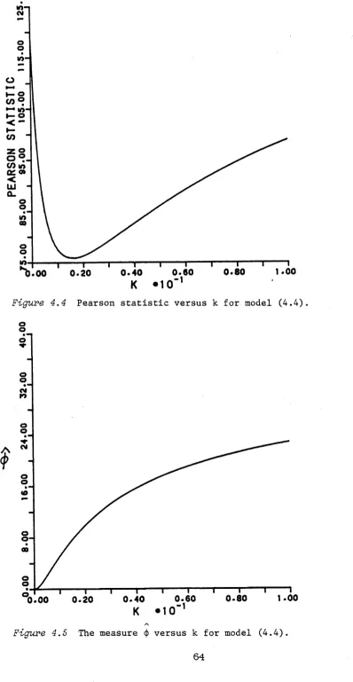
page 68

considered."

page 74 line -6: change "tends" to "may tend" page 78

line 14: delete the words "the plot is essentially linear, indicating that"

page 80

line 12: after "... generally curved", add "relative to the means of the simulations"

page 83

line 10: before "It is easy ...", add "The use of H in logistic regression has been discussed by Pregibon (1981)."

LS line -6 and line -5: change all occurrences of "r" to "r "

page 112 line l: after "Hall.", add

COX, D.R. & HINKLEY, D.V. (1974). Theoretical Statistics. London : Chapman and Hal1.

line 15: after "503-515.", add

FREEMAN, D.H. (1987). Applied Categorical Data Analysis. New York : Marcel Dekker.

page 113 line 14: change "in press" to "233-243"

line 17: change "43, to appear" to "44, in press"

ADDITIONAL REMARKS IN CONNECTION WITH CHAPTER 5

(1) The claim is not that non-linearity (linearity) of the plots implies (no) indication of model inadequacy. Actually, the main claim has been stated on page 75: "If some of the observed values fall beyond or near the boundary of the envelope, then this gives some evidence that the assumptions of the specified GLM do not apply". One is concerned with isolated points and/or the scatter of the sample statistics relative to the mean and envelope of the simulations. If linearity were of primary concern, then this could have incorrectly suggested that model (5.6) might be adequate, for example.

(2) The Normality assumption for lu^ is not important/required due to the inclusion of the simulated means and envelopes, see Williams (1984 and 1987 pl85). The Half-normal plot is used to enhance scaling of the display. See also page 75.

APPENDIX III Soft-tissue Sarcomas Data Analysis

Let us consider the soft-tissue sarcomas data given in Freeman (1987, p84) and reproduced here in Table III.l. The data consist of 524 reports of soft-tissue sarcomas of the arms and legs diagnosed between 1935 and 1974. These reports are classified according to decade of diagnosis and their soft-tissue type. The purpose of the study was to determine whether there is a changing pattern in soft-tissue sarcomas over time.

Decade

Table III.l

Fibroid

Limb Soft-tissue Tissue Type

Lipoid

Sarcomas Data.

Mixed or other

1935-44 40 12 21

case # 1 2 3

1945-54 70 11 31

case # 4 5 6

1955-64 93 38 47

case # 7 8 9

1965-74 43 51 67

case # 10 11 12

Let y . . be the frequency of tumor tissue-type j (j = 1,2 or 3) in decade 2 (T = 1,2,3 or 4). It can be assumed that the responses y .. ” J are independent Poisson variables with means p„ .. If the log-linear

" J model:

log = a + ße + Tfj (III.l)

Table III.2 Log-linear Model Summaries for model (III.l) (a) Full data (b) Case 10 deleted.

a ß2 P3 ß4 tt2 D S

(a) 3.53 (0.126)

0.428 0.891 (0.15) (0.139)

0.791 -0.787 -0.393 (0.141) (0.114) (0.10)

47.46 44.85

(b) 3.71 0.428 (0.126) (0.15)

0.891 (0.139)

1.3 (0.16)

-1.15 -0.754 (0.129) (0.117)

7.98 7.31

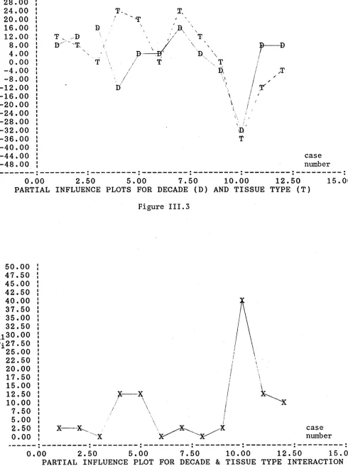
There is strong indication that the main effects model (III.l) might be inadequate for the description of the data. Although there is no general pattern detected in the residual plots of s^ (see Figure III.l and Figure III.2), several large residuals are observed, in particular, s ^ = -3.75. The partial influence plots for decade (ß ) and tissue-type (nr) are given in Figure III.3. It is noted that case 10 with C^q(P) = -32.51 and cj^fTr) = -37.26 can be potentially influential on both decade and tissue-type parameters. However, deletion of this case will only strengthen the significance of ß, as the deviance statistic for ß will be increased to ^ (102.53 - 47.46) + 32.51 = 87.58 (exact value is 86.53). A similar result is found regarding the influence of case 10 on tt. The evidence for both main effects is not dependent on any single case.

To investigate whether tissue-typing is uniform across decades, we add the interaction term to model (III.l):

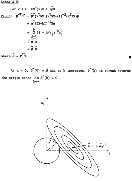
log = a + ߣ + TTj + (P^)^j • (III.2)

which is close to its degrees of freedom. Aside from this one case, no other case seems to be influential. Therefore, it can be established that the evidence for interaction is not spread throughout the data but is dependent on case 10. It is noted that case 10 corresponds to fibroid tumors in the 1965-74 decade. Examination of Table III.1 reveals that, excluding case 10, all three types appear to increase systematically over the four decades. Another observation to be made is the apparent majority of fibroid sarcomas in the first

three decades.

To assess the exact effect of case 10, we refit model (III.l) with this particular case removed. The summary statistics in Table III.2 (b) show that the main effects model now provides a reasonably good fit to the data. There is also no indication from the corresponding partial influence plots (Figure III.5 and Figure III.6) that the evidence for the parameters can be affected by any of the remaining 11 cases. Our analysis therefore suggests that, with the exclusion of fibroid sarcomas in 1965-74, the tissue typing distribution pattern does not change over time. More recent data are clearly needed to support this claim. Finally, since the decade categories are ordered, we can modify the model to take this ordering into account by introducing a decade score d^ = 2-1 to the £th decade group. The resulting simplified model

log Up. = a + ßdp + t

3.600 3.200 2.800 2.400 2.000 1.600 1.200 0.800 0.400 s. 0.000

- 0 . 4 0 0 - 0 . 8 0 0 - 1.200 - 1 . 6 0 0 - 2.000 - 2 . 4 0 0 - 2 . 8 0 0 - 3.200 -3.600 -4.000 -4.400 R RR R R R R R R R R R y

0.0 20.0 4 0 . 0 60. 0 80.0 1 00.0 120.0

P L O T O F R E S I D U A L S V E R S U S Y Figure III.l

3.600 3.200 2.800 2.400 2.000 1.600 1.200 0 . 800 0.400 s 0.000

i-0 . 400 - 0.800 - 1.200 - 1 . 6 0 0 - 2.000 - 2.400 - 2 . 8 0 0 - 3 . 2 0 0 - 3 .600 - 4 .000 - 4.400 R RR R R R R R R R R R A

8.0 24.0 4 0 . 0 56 . 0 72.0 88.0 104.0

P L O T O F R E S I D U A L S V E R S U S F I T T E D V A L U E S

3 2 . 0 0 2 8 . 0 0 2 4 . 0 0

2 0 . 0 0

1 6 . 0 0 1 2 . 0 0 8 . 0 0 1 4 . 0 0 Ci 0 . 0 0

- 4 . 0 0 - 8 . 0 0 - 1 2 . 0 0 - 1 6 . 0 0 - 2 0 . 0 0 - 2 4 . 0 0 - 2 8 . 0 0 - 3 2 . 0 0 - 3 6 . 0 0 - 4 0 . 0 0 - 4 4 . 0 0 - 4 8 . 0 0

T . D

D T.

D

> T

c a s e number

0 . 0 0 2 . 5 0 5 . 0 0 7 . 5 0 1 0 . 0 0 1 2 . 5 0 1 5 . 0 0

PARTIAL INFLUENCE PLOTS FOR DECADE (D ) AND TISSUE TYPE ( T )

F ig u r e I I I . 3

5 0 . 0 0 4 7 . 5 0 4 5 . 0 0 4 2 . 5 0 4 0 . 0 0 3 7 . 5 0 3 5 . 0 0 3 2 . 5 0 i 3 0 . 0 0 c i 2 7 . 5 0 2 5 . 0 0 2 2 . 5 0 2 0 . 0 0 1 7 . 5 0 1 5 . 0 0 1 2 . 5 0 1 0 . 0 0 7 . 5 0 5 . 0 0 2 . 5 0 0 . 0 0

X---X . X

c a s e number

0 . 0 0 2 . 5 0 5 . 0 0 7 . 5 0 1 0 . 0 0 1 2 . 5 0 1 5 . 0 0

Ridge Regression and Diagnostics

in Generalized Linear Models

ANDY HO-WON LEE

A thesis submitted for the degree of Doctor of Philosophy of

The Australian National University

DECLARATION

ACKNOWLEDGEMENTS

I am greatly indebted to my supervisor, Dr Sue R. Wilson, for valuable suggestions, comments, and criticisms throughout the course of my study. Special thanks are also due to Professor Chris C. Heyde for reading and commenting on drafts of this thesis. In addition, I am grateful to Drs Peter Hall, Richard Morton, Mike Osborne, Gordon Smyth, and Neville Weber for many helpful discussions during different stages of my research. In particular, I would like to thank Dr Mervyn Silvapulle who assisted me in the Monte Carlo study in Chapter 4.

ABSTRACT

The first part of this thesis is concerned with the collinearity problem and ridge regression methodology in generalized linear models (GLMs). It is shown that collinearity among the explanatory variables in GLMs may lead to imprecision of the maximum likelihood estimate (MLE), resulting in uncertainty when assessing the effects of the explanatory variables on the response. The conclusion is that inference and variable selection procedures based on the MLE can be noninformative and misleading if the degree of collinearity is sufficiently strong. A ridge type estimator is developed as a suitable supplement to the MLE. Besides theoretical results which indicate that the ridge estimator has smaller mean squared error than the MLE under certain conditions, an empirical study is conducted to evaluate the ridge estimator in practice. It is then observed that for a particular choice of the ridge parameter, the proposed estimator is at least as good as and often much better than the MLE in terms of total and prediction mean squared error criteria. Furthermore, the ridge trace of the estimator will provide a more informative analysis than the maximum likelihood approach alone.

TABLE OF CONTENTS

page

DECLARATION ii

ACKNOWLEDGEMENTS iii

ABSTRACT iv

CHAPTER ONE

1.1. Scope of the thesis 2

1.2. An Overview of GLMs 5

1.3. Asymptotic Properties of the MLE 7

CHAPTER TWO

2.1. Preliminaries 12

2.2. Sources of Collinearity 13

2.3. Detection Diagnostics 16

2.4. Effects of Collinearity 18

2.5. Some Remedies 21

CHAPTER THREE

3.1. Introduction 24

3.2. Ridge Estimation Theory 25

3.3. Existence Theorems 33

3.4. A Bayesian Perspective 38

CHAPTER FOUR

4.1. Optimal and Adaptive Ridge Estimators 44

4.2. Monte Carlo Study 46

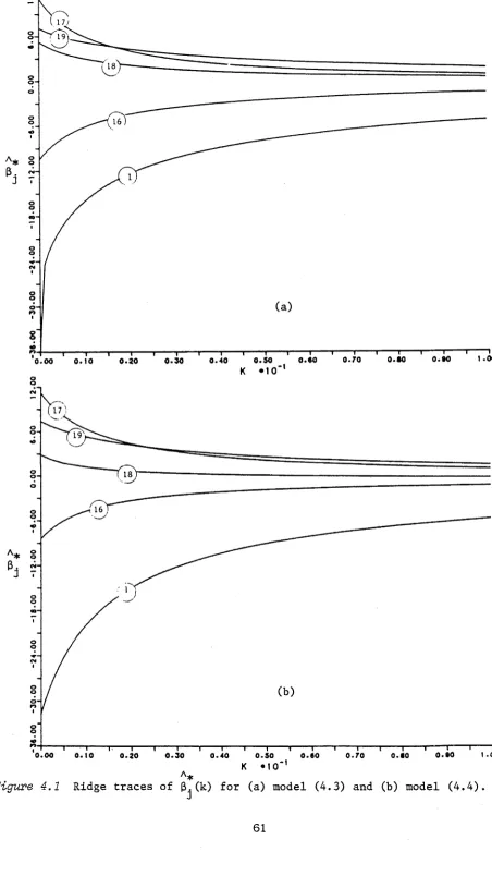
4.3. Ridge Trace Analysis 58

CHAPTER F I V E A S S E S S I N G O V E R A L L L E V E R A G E A N D I N F L U E N C E

5.1. I n t r o d u c t i o n 71

5.2. R e s i d u a l s , L e v e r a g e a n d I n f l u e n c e 71

5.3. G r a p h i c a l D i s p l a y s 7 4

5.4. D e t e c t i n g I n f l u e n t i a l S u b s e t s 8 2

CHAPTER SIX P A R T I A L I N F L U E N C E A N D M O D E L C H E C K I N G D I A G N O S T I C S

6.1. I n t r o d u c t i o n 8 6

6.2. A d d e d V a r i a b l e a n d P a r t i a l R e s i d u a l P l o t s 87

6.3. A s s e s s i n g P a r t i a l I n f l u e n c e 9 0

6.4. A p p l i c a t i o n s a n d E x a m p l e s 9 3

6.5. C o n c l u d i n g R e m a r k s 103

APPENDIX

A p p e n d i x I 106

A p p e n d i x II 110

C H A P T E R O N E

1.1. SCOPE OF THE THESIS

In many applications of generalized linear models (GLMs) introduced by Neider & Wedderburn (1972), the explanatory variables are highly correlated and so are termed collinear or multicol1inear. The problem of col linearity in the linear regression case is well documented and has been studied quite extensively; see eg. Belsley, Kuh & Welsch (1980) and Gunst (1983) for reviews. However, the corresponding problem for other GLMs has not been adequately addressed in the literature. The first part of this thesis is an attempt to fill part of the gap. We shall examine various aspects of the collinearity problem and suggest a supplementary procedure to maximum likelihood estimation that is less affected by collinearity. The proposed method is based on an extension of the ridge estimation

technique to the general framework of GLMs.

It is well known that collinearity can inflate the variance of the least squares estimator in linear regression. Intuitively, one expects a similar problem to occur for other GLMs. Chapter 2 motivates the study of collinearity in the GLM context. We begin with a formal definition of collinearity due to Gunst (1983). Primary sources of collinearity and some of the available detection diagnostics are also reviewed. Next, the adverse effects of collinearity on maximum likelihood estimation in GLMs are examined in detail. We then highlight the advantages and disadvantages of several possible remedies to the problem.

by an existence theorem which shows that the ridge estimator has smaller mean squared error (MSE) than the maximum likelihood estimator (MLE) under certain conditions. A Bayesian perspective of the col linearity problem and a further justification of the ridge estimation procedure are provided at the end of the chapter.

Chapter 4 investigates the performance of the general ridge estimator in practice and the use of the ridge trace plot in GLM data analysis. An empirical study is conducted to determine the MSE properties of two proposed adaptive ridge estimators and to compare these with the MLE under a variety of experimental conditions. Such Monte Carlo experiments are necessary for adaptive ridge estimators due to the mathematical intractability of their sampling properties. Using a set of medical data, it is further illustrated that a ridge

trace of the estimator can provide meaningful estimates in addition to the M L E .

gone unnoticed. Also, graphical diagnostics may suggest appropriate remedial action to correct the problem once it has been detected.

The study of leverage and influence is the topic of Chapter 5. If the fit of a specified GLM depends on one or several observations, the analyst should be made aware of the situation. We call the examination of the dependence of conclusions on particular observations the study of influence. Leverage and influence diagnostic measures will be described. The detection of leverage or extreme design points is important; besides being potentially influential, high leverage observations can induce artificial collinearities among the explanatory variables. A general technique for assessing leverage sind influential observations is proposed. Application of the method is illustrated with an example from logistic regression.

The final chapter is devoted to assessing partial influence in GLMs. We present a unified approach for the detection of individual observations that are influential only on one parameter or a subset of parameters - the so called partial influence assessment. Our general technique is based on analysis using a 'partial influence pl o t ’. Actual examples show that the plot has many potential applications

throughout the model checking procedure. Two other well known diagnostic displays that have been suggested for studying partial

influence are also reviewed.

In the next section of this chapter, we first introduce notation and provide a brief overview of GLMs. Asymptotic properties of the MLE are then examined in Section 1.3. To facilitate subsequent comparison between the MLE and the general ridge estimator in Chapter 3, high order approximations to the bias, variance and MSE expressions

1.2. AN OVERVIEW OF GLMS

Neider & Wedderburn (1972) developed the theory of GLMs to include a wide variety of models found useful in statistical analysis. These include linear regression and analysis-of-variance models, logit and probit models for quantal responses, log-linear models and multinomial response models for counts. An excellent survey of the theory and applications of GLMs is given by McCullagh &. Neider (1983).

The following notation will be used throughout the remainder of this chapter. The observations consist of a vector y of n responses and an n x p matrix X of explanatory variables having full rank p < n. The y^ are assumed to be independent variables with probability

density from the exponential family:

fy.(y:0i ,(^ = exP[(y0i - b(0.)}/a.(<#>) + c.(y,4>)] (1.1)

where a ^ , b and c^ are known functions. Standard log-likelihood calculations yield:

£[y il = M-i = ^(0.) i = ! ___ >n ( i . 2) Var[y.] = v. = b "(0. )a. (<*>) .

(Primes denote differentiation with respect to 0^ and £ stands for expectation.) The function a is commonly of the form (4>)=<J>/(lK ,

being the known prior weight. The dispersion parameter

<t>

2

Exponential variables

<p

\

<p =

Normal variables

<p

o

<p

S Ü ^ ) = # = 17. .

components of 17, the so called composite link relationship (Thompson &. Baker, 1981).

We are interested in estimating

ß

A

estimate (MI.E)

ß

ß

which are in general nonlinear but can be solved by Fisher’s scoring method via:

Neider & Wedderburn (1972) demonstrated that Fisher’s scoring method is equivalent to minimizing the weighted sum of squares:

iteratively with respect to

ß,

This iterative weighted least squares (IWLS) procedure for solving the maximum likelihood equations (1.3) is implemented in the interactive computing package GLIM (Baker & Neider, 1978). It is noted that for Normal linear models, least squares analysis coincides with maximum likelihood estimation; moreover, the log-likelihood is exactly

X^G [y-ji] = 0 ; G = d i a g j v ^

djiVdri^}

where W L J and

p.L

ßL

[y* - Xß]TW[y* - Xß] = [y - n]TV X[y - n]

quadratic so that

ß

2

(i) the deviance D = 2 d . , i=l 1

( 1 - 6 ) (ii) the generalized Pearson statistic S = ^2^s^,

2 ~ 2 Ä

s i = (y i - " d / v i •

McCullagh (1986) derived improved approximations for the conditional distributions of D and S for discrete data. He argued that his conditional cumulant calculations based on Edgeworth expansions are

2

more appropriate than referring to the asymptotic X^n_p ^ limit when the data are sparse.

A

From here onwards, we assume that the MLE ß exists, is finite and unique, and is given by the solution to (1.3). Sometimes it could happen that the MLE does not exist, or exists but is infinite. A simple artificial example for the former case can be found in Press & Wilson (1978). The formal conditions for existence and uniqueness have been discussed in Wedderburn (1976); exact results for Binomial models are provided by Silvapulle (1981).

1.3. ASYMPTOTIC PROPERTIES OF THE MLE

With the exception of Normal linear models, the sampling A

properties of ß cannot be determined exactly. Large sample (n-*») asymptotic results are therefore heavily relied upon. It is assumed that all the necessary regularity conditions (see Fahrmeir & Kaufmann, 1985) have been satisfied. In addition, we make the following assumptions:

(A 1.1) The explanatory variables are bounded, ie. | x_ | ^ x f°r a ^ i ,j , and some finite k.

(A1.2) The diagonal weight matrix W is bounded, ie. |w_ ] < W for all i and some finite W.

(A1.3) lim n *(X^WX) is finite positive definite. n-*°

Assumption (A1.1) makes sense from a practical viewpoint, since

situations. Even if a variable is unbounded for some reason, one can sometimes artifically bound it by a constraint or by way of transformation. From the definition of W in (1.4), Assumption (A1.2) is the same as requiring y to have finite variance and the link function to have finite derivatives, and this is usually the case. The last Assumption (A1.3) is needed to ensure that the asymptotic

A

covariance matrix in the limiting distribution of ß is well defined and has the proper structure. The assumption also implies that the

T

elements of (X WX) are 0(n). It should be noted that (A 1.1) and (A1.2) together do not imply (A1.3) nor vice versa.

Lemma 1.1’ A

The MLE ß is consistent for ß and

1/ Öfl _ 1

n ( P - P ) - Np {0, iß L} (1.7)

where ni„ = X^WX. ß

Proof: see Fahrmeir & Kaufmann (1985). H

Lemma 1.2'

ß is asymptotically sufficient for ß.

Proof: Under mild regularity conditions, the log-likelihood for

ß

log-likelihood, lnL(ß;y), as a Taylor series to second order: lnL(ß;y) = lnL(ß;y) + (ß-ß) [ainL/3ß]~ +

A(ß-ß)T[d2liiL/3ßdßT]~(.ß-ß)

A

consistency of ß for ß,

lnL(ß;y) = lnL(ß;y) - A(ß-ß)T Iß (ß-ß) + 0p (n-14) ,

2 T

where 1^ = £[-c? InL/dßdß = ni^. Exponentiating lnL(ß;y) and approximating I^ by I~ for large n, we obtain:

where L^(y) = L ( ß ; y) does not depend upon ß and L ^ ( ß ; ß ) is A T' HnA /X

proportional to exp[-‘X(ß-ß) X WX(ß-ß)]. The asymptotic sufficiency of ß is thus established by applying the Neyman factorization theorem. ■

For the exponential family (1.1), it has been pointed out (eg. Akahira & Takeuchi (1981), Lehmann (1983, Chp6)) that the MLE ß has bias typically of the form:

8[P - P] = n_1B(P) + 0(n~2 ) , (1.8)

where B(ß) is some function of ß . Furthermore, the covariance matrix

~ -1

and total mean squared error (MSE) of ß to order n are respectively: Cov[ß] = (XTWX)_1 + 0(n~2 ) ,

MSE[ß] = 5(ß-ß)T (ß-ß) = tr{Cov[ß]} + ll£[ß-ß]ll2 = tr{(XTWX)_1} + 0(n~2 ) .

A ('tr* denotes the trace operator.) Note that the squared bias of ß is

-2 -2

0(n ) and thus incorporated within the 0(n ) term in the MSE expression.

In anticipation of future comparisons between the MLE and the general ridge estimator in Chapter 3, a more accurate approximation

_2

(up to o(n )) to the bias, covariance and MSE was judged desirable. The formulae below are presented for this purpose, the proofs of which are outlined in Appendix I.

Lemma 1 . 3 ’

£[ß - ß] = ADI + A A(B1 - hP} + o(n"2 ) (1.9) where

T - I T A = (X WX) X G

D = diag{(32p./ae2 )x^(XTWX)-1(x[)T } , i=l___ ,n

B = diag{( d ^ j i V d d ^ ) x ^ A Cov[t , U l ] A^(x^)^}

fl is an n x p matrix with {(32p V S 0 2 ) x _ t^A^(xT)^x^ At} as its (i,j)th element, and 1 denotes an nxl vector of ones. H

Lemma 1.4:

Cov[ß] = (XTWX)_1 + A(KVar[[71]-Cov[t,Ul])AT + o(n"2 ) (1.10) MSE[ß] = tr{(XTWX)-1} + tr{A(XVar[Ul]-Cov[ t, Ul] )AT }

+ %1TD ATA D1 + o(n'2 ) (1.11) ■

In the derivation of Lemma 1.3, the link function is conveniently taken to be the exponential family canonical parameter, ie. tj = 0^. Canonical links are appealing due to their simplicity and, moreover,

T

there exist sufficient statistics X y for ß so that exact conditional inference concerning the parameters may occasionally be possible. It can be shown that for the special case of binary logistic regression, the first term in (1.9), -lAADl, simplifies to the approximate bias expression given in Amemiya (1980) and Schaefer (1983).

The asymptotic formulae presented above involve quantities which in turn depend on the unknown parameter ß. But in practical applications, such as hypothesis testing and bias correction (ie.

A

correcting ß by its bias), any function of ß can be consistently A

estimated using ß, taking into account the well-known invariance property of the MLE under parametric transformations. For instance,

T -1 . T~

the asymptotic covariance matrix (X WX) may be estimated by (X WX) when drawing inferences/testing hypotheses regarding ß, where denotes W evaluated at ß.

<

C H A P T E R

T W O

2.1. PRELIMINARIES

In this chapter we shall examine various aspects of the collinearity problem. It is instructive to briefly review the definition of collinearity in the least squares regression context. Let us consider the linear regression model:

y = Xß + e , (2.1)

where y is an nxl vector of response variables, X = [x.... x ] is an

1 p

nxp matrix of explanatory variables having full rank p<n, ß is an unknown vector of parameters, and e is a vector of disturbance terms

2

with mean zero and covariance a I. Without loss of generality we

T T

assume that X and y are standardized so that X X and X y contain correlation coefficients of the variables. The following precise definition of collinearity is due to Gunst (1983).

Definition 2. 1 : Consider model (2.1). If for some specified f>0 T

there exists a vector of constants t = ( ' r 1 , . . . , n r ) ?£ 0 such that

1 p

P

2 T.x. = 5 with nail < flltll , (2.2) j=l J J

then a col linearity is said to exist among the (nonconstant)

explanatory variables. B

For this definition to have a practical meaning f must be chosen suitably small, and this choice generally depends on specific features and goals of the analysis. In addition, the above definition allows for the distinction between the existence and the degree of the collinearity. A collinearity is said to exist if and only if (2.2) is satisfied, whereas its degree or strength can be gauged by the magnitude of (11511/llcll). It is noted that the definition also allows for the simultaneous existence of more than one collinearity among the explanatory variables.

to the coordinate in IRP given by the vector t in (2.2). H The direction indicates which explanatory variables are involved in the collinearity as follows. Suppose that (2.2) is satisfied, then some elements of t will be large (in magnitude) relative to the other elements. Those variables associated with large components of nr are highly co11inear and therefore involved in the collinearity. However, the concept of 'harmful’ collinearity is difficult to quantify precisely, as it depends subjectively on the degree of accuracy

required from the particular analysis in question.

In the next section the primary sources of collinearity are summarized, followed in Section 2.3 by techniques of detecting collinearity. The effects of collinearity on maximum likelihood estimation are then examined in Section 2.4. The final section contains comments on remedies to the problem.

2.2. SOURCES OF COLLINEARITY

In GLMs, collinearity among the explanatory variables may be due to a variety of reasons. It is important to differentiate these sources since interpretation and analysis of the data/model depend to some extent on the cause of the problem. Primary sources of collinearities include the following possibilities.

2.2.1 Model Specification

analysis, superfluous explanatory variables are often included in the model since one is uncertain about the relevant predictors. Sometimes these variables may act as a proxy for an unmeasurable quantity or are simultaneously affected by some other covariate/phenomenon and thereby are collinear.

2.2.2 Population-inherent Collinearity

This type of collinearity is due to some inherent characteristic of the population being sampled. For example, blood pressure readings taken from the left (x^) and right arms* measurements on amount of two drugs administered where their combined dosage x^+x^ is restricted to approximately, say, 50 ml. It is the underlying 'physical constraint’ in the population that leads to the collinearity problem. Consequently, collinearity is expected to exist with virtually all the data collected, regardless of the sampling scheme or experimental procedure used to collect the data.

2.2.3 Sampling Deficiency

Many of the collinearity problems encountered in practice are caused by sampling deficiencies. The term 'sampling deficiency’ implies that the sampled covariate values incidentally lie in a subspace of the intended p-dimensional factor/design space; the resulting collinearity is not necessarily due to an inadequate experimental design or a careless sampling technique. The collinearity problem may disappear in similar or subsequently collected data sets. Unlike the previous two sources, substantial bias in coefficient estimates and predictions will occur if one attempts to delete one or more of the collinear variables.

2.2.4 Leverage-induced Collinearity

collinearities - in the sense that deletion of these points eliminates

the associated c o l 1inearity. Let us consider the case p = 2. Suppose

the original design matrix is of the form:

Z = [1. zr z2]

T T

where z^ = (9, z^^, . . . , z ^) • z2 = (k®* z2 2 ... Zn2^ fixed.

As 9 -» 00, the values for the first observation become large relative

to those for the remaining observations. It can be verified that for

the standardized matrix X = [ x - , x^] where

x ij = (zi r V /[i!i(zi j - V 2^'

lim x. . = [(n-l)/n]' 9-*» iJ

lim x = -[(n-l)n]- 1/

j=l ,2

i ^ l , j=l,2.

(2.3)

Consequently, given some prescribed f>0, there exists a value 9q of 9

such that for all 9 > 9q , x^- x^ = 5 with II6II < f, which satisfies

the requirements of Definition 2.1.

For p > 2, using a similar argument on the first q (< p)

nonstandardized variables of the first observation, one can show that

limits analogous to (2.3) hold for the corresponding q explanatory

variables. It then follows that for q sufficiently large Xt can be

made arbitrarily close to 0 for any q-1 orthogonal vectors nr that have constrasts in the first q elements and zeros in the remaining p-q

elements. Thus a q-variate leverage point can induce q-1 linearly

independent collinearities among the corresponding explanatory

variables; see Mason 8i Gunst (1985).

Apparently, a leverage-induced collinearity can exert the

distorting effects of both leverage and collinearity on regression

estimates. A careful examination on the nature of the observed

collinearity is therefore necessary. Identification of leverage

2.3. D E T E C T I O N D I A G N O S T I C S

Various techniques have b e e n proposed for detecting c o l 1i n e a r i t y ,

see eg. M a n s f i e l d & Helms (1982) a nd S t e wart (1987). Some of the

p o p u l a r indicators of collinearity are d e s c r i b e d below.

2.3.1 C o r r e l a t i o n C oefficients

T

Let r .. (= x.x. ) denote the c o r r e l a t i o n coefficient b e t w e e n x.

jk v J k' j

a n d x^, l<j,k<p. As | r ^ | -» 1, a pairwise c o l l i nearity exists b e tween

Xj and x^. Formally, g i v e n some small f > 0,

Xj - s i g n [ r ^ ] x ^ = 5 w i t h IIÖII

so that Definition 2.1 is satisfied wh e n e v e r IIÖII < , or equivalently,

will indicate the strength of the collinearity. However, the

c o l l i nearity of concern m ay involve more than two variables a nd can

exist without a ny of the pairwise c orrelations being large. Thus

inspection of the r .^’s alone is inadequate in most situations.

2 . 3 . 2 E i g e n s y s t e m Analysis

T

Since X X is symmetric, there exists a real pxp orthogonal m a trix

C = ["c... c 1 such that

L 1 p J

T T

(2.4) [2(l-|r.k | ) f .

r I 1 1-f^. The degree to w h i c h Ir.^l exceeds 1

-CT (XT X ) C = A = d i a g l A j ___ ,A }

where 0 < A ^ < ...<A^ denote the ordered eigenvalues of X X, a nd the

columns c ^ , ...,c of C are the ass o c i a t e d eigenvectors w i t h 110^11=1,

k=l,...,p. N o w let us consider the singular-value d e c o m position of X:

iz

x

X = 3fA C

■ I. V k ck

k=l

where .... h ] is a n n xp m a t r i x such that It %

(2.5)

I ; A P l

A lA

d i a g { A ^ ,...,Ap} contains the singular values of X, or square-root of

T

the eigenvalues of X X. It follows from e q u a t i o n (2.5) that:

[c, = 2 c .. x . "k jk j

y %

2 c., x. = 5 w i t h IIÖII = A,

•_1 Jk j

k

w h i c h satisfies Definition 2.1 for the existence of a collinearity

JZ

p r o v i d e d that A ^ < f , in particular that A^ < f. Therefore, an

T

e x a m i n a t i o n of the e igensystem of X X leads to the identification of

one or mor e c o l l i n e a r i t i e s , each associated w ith a sufficiently small

2

(< f ) e i g e nvalue A ^ a nd a d i r ection g i v e n by the eigenvector c^. In

particular, the eignvector c^ specifies the direction where the data

is the least informative. Deter m i n a t i o n of f a g a i n depends on

specific features of the analysis but some guidance can be g i v e n using

the c o n d i t i o n indices of X:

<p . = A /A .

J P J 1 .... P

Belsley, K u h & W e l s c h (1980) argu e d that . is a numerically more

stable m e a s u r e of the degree of collinearity than A. alone. We can

use the con d i t i o n indices to provide an adaptive cut-off value for f.

For example, if one selects a condition index of 10 as an appropriate

lA A

indication of collinearity, then any A, £ f = A /10 signifies the

K p

existence of a c o l l i nearity of sufficient degree.

2 . 3 . 3 O t her Diag n o s t i c s

Several other techniques are available, such as u s ing the

v a r iance inflation factors (Marquardt, 1970) or the determinant of

T

X X. The latter measu r e s the degree of the collinearity but fails to

T H

reveal the variables involved; note that 0 < det[X X] =11 A. < 1. j=i J

Another useful d iagnostic is the ridge trace display w h i c h depicts

changes in the p a r a meter estimates through slight perturbations in the

data. T h ose variables that are collinear will exhibit instability

and/or large fluctuations in the trace of their corresponding

estimated coefficients. This ridge trace procedure will be

2.4. EFFECTS OF COLLINEARITY

It is well known that col linearity inflates the variance of the

least squares estimator in linear regression. Consider the least

squares estimator for model (2.1):

~ T -1 T

P

Using (2.4), (X^X) ^ can be written as:

(2 .6 )

,T,„-1 -1

(XX)

= 2

k=l

so that

/V A

2rvTv ^ j 2? .-1

Cov[ß^,ß.] = a (X X) J = ^ ^ ‘c ^ C j k £.1=1.--- P,

k=l

where ( X ^ X ) ^ denotes the (£,j) entry of (X^X) ^ Suppose and x^.

are involved in the collinearity as characterized by -* 0, then c ^

and c ^ will be large yielding inflated variances and covariances for

/V A

ß^ and ß y To examine the effects of collinearity on maximum

likelihood estimation, we assume initially that there exists only one

collinearity among the explanatory variables. In particular, suppose

that the jth column x^. is closely approximated by a linear combination

of the remaining columns of X. If we partition X into [x^. |X^.^] where

X^. j is the nx(p-l) matrix obtained by deleting x^., then the residual x .- X, .> b . where

J (j) J

vector from regressing x^. on X^. ^ is given by 5^.

T - I T

bj = X ^ . ^ X j . Hence, given some specified f > 0, provided

that

(ö^öj)^

f(l+b^bj)

collinearity will be satisfied. The degree of the collinearity

T -1

increases as Ö.Ö. -> 0. Let us consider the asymptotic (to 0(n )) J <3

diaglv.^aji./ai^)2 } covariance matrix of ß:

Acov[ß] = (XTWX)_1 ; V

Theorem 2.1• T

As 5.5. -* 0, Avar[ß.] -» °°. 1

A

( X ^ W X ) ^ . Using the partitioned matrix inversion result (see eg.

Atkinson (1985, p.272)), it can be verified that:

(XT WX)JJ =

[xjwx.

Substituting X ^ . f o r x^. into (2.7), and expanding and cancelling

terms, we obtain:

(XTW X ) JJ= [öjtfö ] l; * W-WX, .,(XrT AWX, . J \ T.JI .

(j)v (j) (j

)7

(j)

Since ^ is symmetric, there exists a real nxn orthogonal matrix U

fu.,,...,u 1 such that

^ 1 n J

UT W = A = diag{X.} ,

where A- , . . . ,X denote the eigenvalues of and the columns u.

l n 0 I n

of U are the associated eigenvectors with llujl

let a . = U 5 . and X = max |X. I, then

j j max „ ,. , 1 l 1

, . . . ,u r

1, i= l.... n. If we

l<i<n

| ö Tt f ö .

1 J J

'-rv'vv

Ia .Aa.

J J

illX ia ji

< A 2 a T .

max. ji

1=1

~ T

X 5.5. .

max j j

By assumptions (A 1.1) and (A1.2), X and W are bounded, implying that

X is bounded as well. Hence |[öT'frö.] ^ I > A ^ (Ö^Ö.) ^ . As

max J J max j j'

ÖT Ö. -► 0, Avar[ß .] = [öTtfö .]-1-> <». u

J J 3 3 1

Theorem 2 . 2 :

<"p A A

As Öjöj -> 0, Acov[ß^,ßj] 00 for all £■£j .

Proof: This is evident from the fact that the asymptotic covariance

(X WX) ^ can be written as [5.#5.] s^ where s^ is the £th element of

s = -[X,TaWX, . J -1X rT ,Wx.

L O) O r

(

)

= -b.-[XrT ,WXr . J -1X,TaWÖ.

j

L O) O r

O)

T

and s is bounded away from 0, | s | -» |b^. | >0, as 5^.5^. 0. ■

It then follows that if there exists one or more collinearities

imprecise and may not reflect the actual effects of the explanatory variables. Furthermore, it is clear that

MSE[ß] = 2 (XTWX)JJ + 0(n 2 ) j=l

will also be large. The above arguments will still apply when W is

A A

estimated by W = W(ß). Both actual examples and empirical studies indeed confirm this to be the case; see Schaefer (1986), Lee & Silvapulle (1987) and Chapter 4 of this thesis.

In addition to the precision problem, the estimates themselves may be directly affected by collinearity. For the linear regression case, the least squares estimator (2.6) can be expressed as:

ß = C A ~ V y = 2

\ \ ° k

(2.8)

k=l

where

v^=

l

A

*

value X. will tend to dominate those ß . ’s associated with col linear

k J

variables (ie. those having large c., ’s). This implies that coefficient estimates for collinear variables could possess large magnitudes and their sign patterns are determined by the direction of the collinearity and not through the relationships between the explanatory variables and the response. For other GLMs, there is no A closed form expression similar to (2.8) available for the MLE ß. Nevertheless, the Fisher’s scoring/IWLS procedure may fail to converge as a result of severe collinearity. From Section 1.2, the iterative process of solving ß is consisted of:

p[<+1L pW

T -1

It has been shown that (X WX) contains large elements for a sufficient degree of collinearity, The same arguments apply to

[«]

T - m -i

(X W L JX) based on any estimate ß L . Hence the remainder term A T - m

2.5. SOME REMEDIES 2.5.1 Variable Deletion

One suggestion for dealing with population-inherent collinearity is to delete one or more of the highly col linear variables, so that the degree and effects of the corresponding collinearity are thereby reduced. The explanatory variable(s) eliminated may perhaps be compensated for by other variables with which they are collinear. For other sources of collinearity (especially sampling deficiency), variable deletion is not recommended. This method deletes a variable based solely on its interdependence with other explanatory variables but not on its relationship to the response. The reduced model could result in having low predictive power if the explanatory variable dropped does in fact have an important effect on the response.

2.5.2 Data Augmentation

By collecting more data, the problem of sampling deficient collinearity may possibly be alleviated, thus enabling acceptable parametric estimation via maximum likelihood. However in most observational studies, it is often infeasible to collect more data or perform further sampling due to economic, time and other constraints. Even when additional data are available, the extra observations could either extend beyond the range of the original variables or be atypical of the underlying process and hence inappropriate to be included. Finally, it should be clear that data augmentation cannot overcome the problem of population-inherent collinearity.

2.5.3 Biased Estimation Methods

a new interpretation of the data that has not been previously considered, and in turn, lead to a better understanding of the process under study.

C H A P T E R T H R E E

3.1. INTRODUCTION

In this chapter the ridge estimation methodology for GLMs is proposed to deal with the collinearity problem. The underlying theory is an extension of the ridge estimation approach used by Hoerl & Kennard (1970a) in least squares regression. Furthermore, the proposed estimator includes the 'ridge logistic estimator* of Schaefer, Roi &. Wolfe (1984) as a special case.

It was shown in Section 2.4 that if there exists one collinearity or more of sufficient degree, some of the maximum likelihood estimates

A A

ß j ’s will be imprecise and consequently, MSE[ß] will also be large, A

meaning that ß is far removed from the true ß in the MSE sense. Moreover, since

Cov[ß] = g(ß - Sß)(ß - gß)T = (XTWX)_1 + 0(n"2 ) , taking trace of both sides yields:

tr[£(P ~ SP)(P ~

= g[Cr(p -

Sß)T ]

=

H P - sp)T {P ~ SP)

= *(ßAß) - (Sß)l(gß)

= J.|1(XTWX)JJ + 0(n~2 ) . vA. 'y* A

But (£ß) (£ß) is positive and hence Theorem 2.1 implies that

£(ßTß) > j.|1(XTWX)JJ oo as ÖT.Ö. 0, A

ie. Ilßll will be too large on the average. These undesirable features A

of ß in the event of collinearity motivate the development of an A

improved estimator which (i) hopefully is closer to ß than is ß in the MSE sense and (ii) simultaneously satisfies the criterion of smaller

A norm than ß.

interpretations of this new estimator, its asymptotic properties are then examined in detail. In Section 3.3, an existence theorem which shows that the ridge estimator has smaller MSE than the MLE under certain conditions is proposed and proved. A Bayesian formulation of the collinearity problem and a further justification of the ridge estimation procedure are given in the last section. Throughout this chapter, we shall make use of the orthogonal decomposition of the information matrix I^ = (X WX) :

PT (XTWX)P = E = diag{e.} (3.1)

where e^<...<e^ denote the ordered eigenvalues of X WX, and the columns of P are the associated eigenvectors with IIt^II = 1, k = 1,...,p.

3.2. RIDGE ESTIMATION THEORY 3.2.1 General Ridge Estimator

Suppose a new estimator ß is sought based solely on the minimum norm criterion, the resulting estimator, ß = 0, is unacceptable.

A

Although it trivially has smaller norm than ß, it does not provide any information about ß. Some additional constraint must be imposed in order to produce a meaningful estimate.

Definition 3.1’ Let ß be any estimator of ß. The Weighted Sum of Squares function is defined as:

WSS(P) =

[y - n(ß)]V1[y - n(ß)]

where V is fixed at ß. ■

Recall from Section 1.2 that the maximum likelihood equations may be solved via the IWLS procedure by minimizing WSS(ß) iteratively with

A

respect to ß. The solution, ß, may be regarded as 'optimal’ in terms of this WSS. Any other reasonable estimator ß should therefore be

Definition 3 . 2 : The closeness between an estimator ß and the MT.F. ß is:

< k h = WSS(P) - WSS(P) . ,

This closeness criterion will provide an additional constraint in deriving a new estimator for ß. Let us consider the first order approximation (j) of (j).

Lemma 3.1'

If ß is consistent for ß, then

I4KP) - 4>l ^ o ,

where $ = (P - P)TXTWX(P - P) .

A /V A

Proof: Denoting p(ß) and p(ß) by p and p respectively and observing

A/ A A A*

that y-p = y-p+p-p, it can be verified easily that:

A* yv /A* rp -j A Ay yV A» T» ■% yv

4XP) = [P - p] v [p - p] + 2[p - p] V [y - p] .

A /%/

Since ß and ß are both consistent for ß, first order Taylor series

A A/

expansions of p and p about ß give: h = h + VGX(p-p) + op (n_1/} ü = H + VGX(P-P) + o (n-14) . This implies that

<t>= [VGX(P-P)]TV_1[VGX(P-P)] + 2[VGX(p-p)]TV _1[y-jz] + op (n_i4) = (p-p) X GVGX(p-p) + 2(p-p)1X 1G[y-n] + o (n .

.H

As GVG = W and X^G[y-p] = 0 , |({) - (ß-ß)^X^WX(ß-ß) | ^ 0 as required, h

The measure may be interpreted as the asymptotic confidence

A

region displacement from ß. Restricting our attention to the class of A/

consistent and shrinkage estimators ß (ie. having shorter length than yv

ß ) , a ridge type estimator for GLMs can be obtained as follows. Lemma 3.2:

The estimator ß that has minimum squared norm subject to

(3.2) ß* = (XT WX + kl) X (XT WX) ß

/ » /v»

w h e r e k > 0 is chosen to satisfy the constraint <() = <()

Proof: This can be established by minimizing:

F(P) = PP + k [(P-P)VWX(P-P) - (

J

)

o]

w i t h respect to ß, where k ^ denotes the Lagrange multiplier.

C o n s i d e r :

dF/dß = 2ß + k _ 1 [2XTWX(ß-ß)]

d^F/dßdß1 = 21 + 2k _ 1 (XT WX) .

c y a» /'»■p

For k>0, the h e s s i a n m a t r i x 3 F/dßdß is positive definite an d hence a

A /

local m i n i m u m of F exists w h i c h is g i ven by setting dF/dß to 0. This

y i e l d s ß as in (3.2) w i t h k satisfying:

(P-P*)T XT WX(P-P*) = $ o . (3.3)

We a re not interested in the case k<0 as this will not correspond to

the class of shrinkage estimators.

To solve for k, one substitutes the expression (3.2) for

ß

(3.3), yielding:

cb = { [ I - ( X AWX+kI) 1XT WX]ß}T XT WX { [ I - ( X iWX+kI) T, - L X

Vwx]ß>

= k 2ßT (XT WX+kI) 1X TW X (X T W X + k I ) lß

since I-(XTW X + k I ) _1XT W X = k (XT W X + k I ) _ 1 .

(3.4)

U s i n g (3.1), (X^WX+kl) P(E+kI) a nd thus (3.4) may be w r itten as

$ o = k 2aT (E + k I ) ~ 1E ( E + k I ) ' 1a

= k 2 I e . a 2/ ( e . + k ) 2 ,

J — i J J J

a t~ P A2 2

w h ere a = P ß. The function f(k) = j2^e^.a^./(l+e^./k) is monotone

P ~ 2

increasing from f(0) = 0 to lim f(k) = .2..e.a.. Therefore there

^ J J

exists a unique positive root k Q say as the solution to the nonlinear

eq u a t i o n (3.3) p r o vided that (J)o < .E.e.a.. The corresponding

An alternative derivation of ß is given in the next Lemma, the proof of which is similar to that of Lemma 3.2.

Lemma 3. 3 :

~ 2 2 AT A *

If the squared norm of ß is fixed at r , 0 < r < ß ß, then ß is » v

the value of ß that gives a minimum asymptotic confidence ellipsoid displacement (p, where k>0 is now chosen so that ß ß = r . H

$4

Definition 3 . 3 : The general ridge estimator for GLMs is:

ß*(k) = (XTWX+kI)_1(XTWX)ß (3.5)

where the scalar k is called the ridge parameter. H The dependence of the general ridge estimator on k is clearly emphasized in the above definition. Furthermore, the estimator (3.5) can be considered as a generalized version of the ordinary ridge estimator of Hoerl & Kennard (1970a). For the special case of binary logistic regression, it is also easy to show that the estimator simplifies to the 'ridge logistic estimator* of Schaefer, Roi & Wolfe

(1984). Lemma 3.4:

For the Normal linear model with identity link =

xTß,

ß*(k) = (XTX+kI)_1XTy . (3.6)

~ T -1 T Proof: The MLE and least squares estimator here is ß = (X X) X y. Assuming without loss of generality that the prior weights gj = 1 for all i and <j> = , the information matrix X^WX simplifies to a ^X^X. Thus,

ß* = (a"2XTX+kI)_1cr"2XTX(XTX)"1XTy

= ( X^X+cr^k I) ~ 1 XTy = (XTX+kI)_1XTy