Tolling, Capacity Selection and Equilibrium Problems with Equilibrium Constraints

promoting access to White Rose research papers

Universities of Leeds, Sheffield and York

http://eprints.whiterose.ac.uk/

White Rose Research Online URL for this paper: http://eprints.whiterose.ac.uk/4051/

Conference paper

Koh, Andrew and Shepherd, Simon (2008) Tolling, Capacity Selection and Equilibrium Problems with Equilibrium Constraints. In: 3rd Kuhmo-Nectar

Tolling, Capacity Selection and Equilibrium Problems with

Equilibrium Constraints

Paper for the 3rd Kuhmo-Nectar Conference, Free University of Amsterdam, July 3 – 4, 2008

Andrew Koh and Simon Shepherd Institute for Transport Studies University of Leeds,

Leeds, LS2 9JT, United Kingdom

[email protected] [email protected]

Abstract:

An Equilibrium problem with an equilibrium constraint is a mathematical construct that can be applied to private competition in highway networks. In this paper we consider the problem of finding a Nash Equilibrium regarding competition in toll pricing on a network utilising 2 alternative algorithms. In the first algorithm, we utilise a Gauss Siedel fixed point approach based on the cutting constraint algorithm for toll pricing. In the second algorithm, we extend an existing sequential linear complementarity approach for finding Nash equilibrium subject to Wardrop Equilibrium constraints. Finally we consider how the equilibrium may change between the Nash competitive equilibrium and a collusive equilibrium where the two players co-operate to form the equivalent of a monopoly operation.

KEY WORDS: EPECS, Competition, Diagonalisation, Nash Equilibrium

JEL CODES: C72 (Non Cooperative Games), R42 (Government and Private Investment Analysis), R48 (Government Pricing; Regulatory Policies)

1.

INTRODUCTION

The motivation of the research in this paper stems from the observation that in recent years there has been increasing amount of private sector participation within areas that are conventionally the privy of the public purse. The driving force behind this change is brought about the higher efficiency of the private sector coupled with increasing public pressures on governments for accountability and the corresponding need to derive value for money from their various budgetary commitments which are ultimately funded by the tax paying public.

In highway transportation, privately operated roads are not novel concepts [1]. However there has been little analysis on this topic in terms of the competition between private sector providers and the equilibrium outcomes, save for theoretical studies by economists restricted to simplified networks (e.g. [2]). In reality, there have already been examples of private sector involvement in road construction and operation around the world [3]. In return for the private capitalists funding large amounts of initial capital investments for the construction of the road, they are contractually allowed to collect tolls, for some agreed duration from users when the road is finally opened [4]. In an era when government budgets are becoming increasingly tight and with traffic congestion becoming more of a problem in many major cities, the private sector is recognised as having an increasing role to play in the provision of traditional highway transportation investment. When the private sector is tasked with the provision of such services and in competition with others simultaneously doing the same, the concept of Nash equilibrium [5] can be used to model the equilibrium decision variables offered to the market.

In addition, we consider the effect of collusion in the setting of tolls and propose an intuitive structure which allows this response to be modelled.

The structure of this paper is as follows. Next we define in detail the problem that we consider in this paper along with the concept of Nash Equilibrium from [5] which serves as the foundation for the type of non cooperative games that we discuss. Section 3 then develops two heuristic algorithms for the problem. Section 4 utilises two numerical examples to illustrate the performance of the algorithm. In Section 5 we relax the notion of non-cooperative behaviour and consider if it is possible for the players to signal, through their selection of strategic variables, to their competitor, their intention to collude such that they end up in a monopolistic equilibrium. Finally in Section 6, we summarise our results and provide directions for further research.

2.

Problem Definition

Our problem is to find an optimal equilibrium toll and/or link capacity for each private operator1 who separately controls a predefined link on the traffic network under consideration. We can consider this problem to be a Cournot Nash game between these individual operators. The equilibrium decision variables can be determined using the concept of Nash equilibrium [5] which we define as follows:

Nash Equilibrium

In a single shot normal form game with N players indexed by i,j∈{1,2,...,N}, each player

can play a strategy ui∈Ui which all players are assumed to announce simultaneously. Let

1 2

( , ,..., N)

u= u u u ∈U be the combined strategy space of all players in this game and let

( )

i u

ψ be some payoff or profit function to i∈{1,2,...,N} player if the combined strategy is

played. The combined strategy tuple is a Nash Equilibrium * _{( , ,...,1}* *₂ *₎

N

u = u u u ∈U for the

game if the following holds

1 _{As the research transcends both game theory and market structures in the context of highway}

* * * *

( , ) ( , ) , , {1, 2,... },

i u ui j i u ui j ui Ui i j N i j

ψ ≥ψ ∀ ∈ ∀ ∈ ≠ (1)

Equation (1) states that a Nash equilibrium is attained when no player in the game has an incentive to deviate from his current strategy. She is therefore doing the best she can given what her competitors are doing [6].

Problem Definition

We now outline the problem we wish to solve as viewed by each operator with equilibrium conditions imposed on the users’ route choice.

Define:

A: the set of directed links in a traffic network,

B: the set of links which have their tolls and capacities optimised, B⊂A K: the set of origin destination (O-D) pairs in the network

v: the vector of link flows v=[ ],v_a a∈A

β: the vector of link capacities β=[ ],βa a∈B

τ: the vector of link tolls τ=[ ],τa a∈B

c(v,β): the vector of monotonically non decreasing travel costs as a function of link flows

[ ( ,c va a βa)],a A

= ∈

c

μ: the vector of generalized travel cost for each OD pair μ=[ ],μk k∈K

d: the continuous and monotonically decreasing demand function for each O-D pair as a function of the generalized travel cost between OD pairkalone, d=[ ],dk k∈K and

−1

D : the inverse demand function

Ω: feasible region of flow vectors, (defined by a linear equation system of flow conservation constraints).

( )i

If we assume that each player controls2 only a single link in the network then, following Yang et al [7], the optimisation problem for each player, which represents the profit for the operator after investment costs of capacity3 is formulated as follows:

, ( ) ( ) ( ),

Max

i i

i vi i I i i N

τ β ψ τ,β = τ,βτ θ β− ∀ ∈ (2)

Where viis obtained by solving the variational inequality (see [8]-[9])

(

) (

)

(

) (

)

( )

c v τ,β v v D d τ,β d d v d Ω (3)

The objective for each firm (payoff) is the difference between the toll revenue obtained

by charging tolls on links operated by the th

i player and the investment cost of capacity.

The scalar θ allows for an easy conversion of the investment cost of capacity via the investment function from money values into time.

Note that the vector of link flows can only be obtained by solving the variational inequality given by (3). This variational inequality represents Wardrop’s user equilibrium condition which states that no road user on the network can unilaterally benefit by changing routes at the equilibrium [10]. Throughout this paper, we make the additional simplifying assumption that the travel cost of any link in the network is dependent only on flow on the link itself so that the above variational inequality in (3) can be solved by means of a convex optimisation problem [11].

In the case when we have operators who compete only in maximising their revenues by charging tolls then the payoff function for each player would be the toll revenue alone and this is given by

( ) ( ) ,

i vi i i N

ψ τ,β = τ,βτ ∀ ∈ (4)

2 _{Control is used as a short hand to imply that the firm has been awarded some franchise for operating the}

link.

together with the constraint as in (3) above.

3.

Two Heuristic Algorithms for EPECs

The problem we have defined in the foregoing is in fact an Equilibrium Problem with Equilibrium Constraints (EPEC) [12]. In essence these are problems of finding equilibrium points when the constraints define the overall system equilibrium. The study of EPECs has only just recently surfaced as an important research area within a field of mathematics but has significant practical applications elsewhere.

While algorithms with convergence proofs have been proposed recently for EPECs ([13]-[14]), they have not been applied to problems that occur within transportation. In this paper, we propose two alternative heuristics for the resolution of the problem.

The first algorithm is the diagonalisation algorithm which is a modified version of the non linear Gauss-Siedel method (as discussed in e.g. [15]-[16]). The second algorithm is a heuristic derived from reformulating the standard Cournot Nash game from economics as a complementarity problem and solving it using a sequential linear complementarity programming approach. Note that the diagonalisation algorithm can be used for both simultaneous toll and capacity selection as well as toll level selection only while the second approach is restricted to the toll level selection problem only.

Diagonalisation Algorithm (Algorithm 1)

Hobbs et al [19] have used the diagonalisation algorithm to solve EPECs arising in the deregulated electricity markets.

The algorithm is presented as follows:

DIAGONALISATION ALGORITHM

Step 0: Set iteration counterk=0. Select a convergence tolerance parameter,

ε(ε>0). Choose a strategy for each player. Let the initial strategy set be denoted uk =( , ,...,u u₁k 2k uk_N). Set k= +k 1and go to Step 2,

Step 1: For the ith player i∈{1,2,...,N}, solve the following optimization

problem:

1 _{max ( , ) , {1, 2,... },}

i i

k k

i i i j

u U

u + ψ u u i j N i j

∈

= ∀ ∈ ≠

Step 2:

If 1 1

N

k k i i i

u + u ε

=

− ≤

∑

In step 1, we utilise the Cutting Constraint Algorithm (CCA) [20] to solve the optimisation problem for each player holding the other player’s strategic variables fixed. Further details regarding the CCA are provided in the appendix to this paper.

The convergence proof of the Diagonalisation algorithm when applied to single level Nash equilibrium problems can be found in [21]- [22]. However the proofs depend on certain conditions that may not be satisfied in an EPEC, particularly the concavity of payoff functions. In fact, convergence of the algorithm relies on the concept of diagonal dominance of the Jacobians of the payoff functions [23]4, which intuitively implies that a player has more control over his payoff functions than do his competitors. Therefore we propose this algorithm to be a heuristic approach for the EPEC at hand.

Sequential Linear Complementarity Problem Algorithm (Algorithm 2)

Since the game between the operators in this paper is akin to a Cournot Nash game, the second algorithm reformulates the Cournot Nash game as a complementarity problem. Adopting this approach, Kolstad and Matthisen [24] developed a sequential linear complementarity problem (SLCP) approach to solve the resulting reformulation. At each iteration, the main problem is linearised (using a first order Taylor expansion) at a given starting point. Then the sub problem is solved as a linear complementarity problem for which the algorithm of Lemke [25] can be applied. As far as we are aware, this is the first application of the algorithm to the EPEC.

To demonstrate the approach, recall that the profits of the firmi is given by (4). The first

order conditions of a profit maximum for each firm are therefore given by (5)-(7) as follows :- 0 i i i f ψ τ ∂ = − ≥

∂ (5)

0 i i i ψ τ τ ∂ ₌

∂ (6)

0

i

τ ≥ (7)

Note that these first order conditions define a complementarity problem (CP) as characterized by the system given in (8):

Find _τ N

+

∈ℜ given : N N

f R₊ →R such that

( ) 0 ( ) 0

0 T _τ ≥ ≥ ≥ f τ τ f τ (8)

If we denote the linearization of f at τ0(some arbitrary starting vector of tolls) using the

first order Taylor expansion, then we obtain _{( /} 0_{) ( )}0 _{( )(}0 0₎

following [24], the resulting Linear Complementarity Problem (LCP) is to find

j

τ∈ℜ+ such that

0

( / ) , 0

( ) 0

T

Lf q M

q M

τ τ τ

τ

τ τ

= + ≥

+ =

(9)

Where _{q= f( )τ}0 _{− ∇f( )τ τ}0 0 _{andM = ∇f( )τ}0

In summary the proposed algorithm is as follows

SEQUENTIAL LINEAR COMPLEMENTARITY PROBLEM ALGORITHM

Step 0: Choose some starting vector of tolls _τ0_{. Select a}

convergence tolerance parameter, ε(ε>0), and set

1

k= +k and go to Step 2,

Step 1: Use finite differencing approximation to obtain _f( )_τk

and _∇f( )τk

Step 2: Solve the LCP (9) to obtain _τk+1

Step 3: _{Check convergence: If maximum of f(τ}k+1_{) <ε} ,

terminate else set k= +k 1 and go to Step 1

Note that in order to solve the LCP, we require both the Jacobian of the profit function

( )k

f τ for each firm in the game at iteration kand the Hessian (M ). To do so, we solve a

traffic assignment problem at _τkand perturb the tolls by using the method of central

differences (forward and backward) to approximate the gradients. The underlying assumption here is that the derivatives exist and can be approximated in this way.

As with the diagonalisation approach, the convergence proof of this algorithm relies specifically on the concavity of the payoff functions of each firm [24]5. While this assumption is usually acceptable in modelling the classical Cournot Nash game for which it was developed, it may not be satisfied in a general EPEC setting. Furthermore we have made use of finite differencing to obtain derivatives. For these reasons, therefore, our proposed algorithm is to be viewed as a heuristic. In terms of implementation, to solve the SLCP in Step 2, we used the PATH solver [26] within MATLAB.

4.

Numerical Examples

In this section, we provide two examples of how the proposed heuristics are used to solve for the optimal tolls and capacity. In addition, we compare the equilibrium outputs under the scenarios of competition, monopoly and under the objective of (second best) social welfare maximisation.

In the case of monopoly, we assume that the there is a single private operator controlling the predefined links in the network. Hence this is a simpler problem that can be solved directly using the CCA (see Appendix A) or any derivative free direct search method (e.g. Hooke Jeeves direct search [27] or Nelder Mead Simplex algorithm [28]). For the results presented here, the CCA was utilised.

In the case of social welfare maximisation, the central planner solves the following problem.

( )

1 0

Max ( ) ( )

. . , 0

k

d

a a a k K a A

d x c v v

s t τ

τ τ

−

∈ ∈

−

∈ Ω ≤ ≤

∑

∫

∑

v d

(10)

Where τ is the pre-specified upper bound on tolls on tolled links, τ =[ ],τ_a a∈B. The CCA

algorithm can be utilised for this problem.

Example 1

The first example is taken from [29]. The link specific parameters and the elastic demand functions can be found therein. This network has 18 one way links with 6 origin destination pairs (1 to 5, 1 to 7, 5 to 1, 5 to 7, 7 to 1 and 7 to 5).

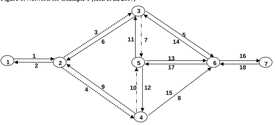
Two separate scenarios are considered in this numerical example. In Scenario 1, Links 3 and 4 shown as dashed lines in Figure 1 are the only links in this network that are subject to tolls. In Scenario 2, Links 7 and 10 shown in an alternative style of dashed links represent the only links subject to tolls in the network. Note that in all which follows we set the maximum allowable toll to be 1000 seconds.

Figure 1: Network for Example 1 (Koh et al, 2007)

1 2

3

6 11 7

9 4

5 14

13 17

16

18

15 8 10 12

1 2 5

3

4

Table 1: Comparing Solution by Alternative Algorithms for Example 1 [29]. (Tolls in seconds)

Algorithm Diagonalisation6 _SLCP7

Toll Iterations Iterations

Scenario 1 Link 3 530.63 25 530.55 6

Link 4 505.65 505.62

Scenario 2 Link 7 141.37 25 141.36 6

Link 10 138.29 138.29

Table 1shows the resulting tolls and number of iterations required for each algorithm for the Nash solution. As shown the resulting tolls are almost identical and any differences are due to the convergence criteria used. SLCP uses fewer iterations as it does not rely on a diagonalisation approach and this would suggest the algorithm is more efficient.

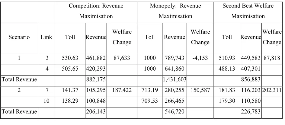
Table 2 shows the tolls, revenues collected and the change in social welfare for each toll pair under (a) the competitive case, (b) the monopoly case and (c) the second-best welfare case where operators are assumed to co-operate to maximise social welfare.

Table 2: Tolls, Revenues and Welfare Changes under Alternative Market Structure Assumptions (Tolls in seconds, Revenue and Welfare in seconds/hr)

Competition: Revenue Maximisation

Monopoly: Revenue Maximisation

Second Best Welfare Maximisation

Scenario Link Toll Revenue Welfare

Change Toll Revenue

Welfare

Change Toll Revenue

Welfare Change

1 3 530.63 461,882 87,633 1000 789,743 -4,153 510.93 449,583 87,818

4 505.65 420,293 1000 641,860 488.13 407,301

Total Revenue 882,175 1,431,603 856,883

2 7 141.37 105,295 187,422 713.19 280,255 150,587 181.83 116,203 202,311

10 138.29 100,848 709.53 266,465 179.30 110,580

Total Revenue 206,143 546,720 226,783

6 _{Using the diagonalisation algorithm with CCA and a termination tolerance of ε = 1e-06.}

Table 2 shows that when there are no alternative routes available (as in the case of Scenario 1 where Links 3 and 4 are tolled), the monopolist can charge the maximum toll allowable. In fact the upper bound of the toll here is a binding constraint on the revenues in the monopoly case. However in the case of two competing operators, each player has no alternative but to succumb to the strategy charged by the other and hence ultimately both are only able to charge a much lower toll (50% lower than the monopolist’s toll).

The overall welfare change for Scenario 1 under competition in fact approximates that of second best social welfare maximisation. It is also clear that as expected society as a whole is worse off under monopoly.

The more interesting case emerges in Scenario 2 when there is an alternative link available for travel into destination Zone 5 which is left untolled (Link 17) in Figure 1. Even the monopolist controlling Links 7 and 10 together cannot charge the maximum allowed toll of 1000 seconds on each link to maximise his revenue. In the case of competition, Table 2 shows that the tolls charged and the total revenue earned are even lower than that under that of a central planner attempting to maximise social welfare in a second best case. It is an interesting observation here that the competition has the effect of driving tolls down below the socially optimal level. However the change in social welfare is also lower under competition.

INDEXOFRELATIVEWELFAREIMPROVEMENT

Table 3: Index of Relative Welfare Improvement under alternative scenarios

Test Pair Competition Monopoly Second Best Welfare Maximisation

Scenario 1 0.19 -0.01 0.19

Scenario 2 0.41 0.33 0.44

This enables us to confirm that the welfare gains under second best welfare maximisation and under competition for both scenarios are similar.

Example 2

Our next example is based on a network with 4 OD pairs and 11 one way links with parameters taken from Yang et al [7]. In this example there are 3 players, each controlling a single link on the network shown in Figure 2.

Figure 2: Network for Example 2 [7]

1 4

1

3

7

5

4 2

5

2 6 8

6

3

7

10

11

In the problem setting, players simultaneously optimise both tolls and capacity to maximise total profit as given by equation (2). In particular, θis given as 0.114 which is common to all players and the investment cost functions take the formI( )βi =t0,iβi. In

other words, the investment cost is dependent on the free flow travel time (t0,i) for each

link. The free flow times for the 3 links 9, 10 and 11 (shown as dashed lines in Figure 2) are 11,11 and 15 secs respectively.

Full details of the link parameters and the OD (with elastic demands) can be found in [7]. In that paper, the authors employed a heuristic based on sensitivity analysis to solve this problem. The comparison against monopoly and competitive situations can be found in [7] and are not reproduced here.

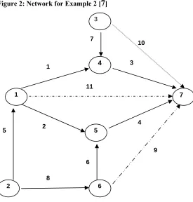
For reasons mentioned above we have not been able to implement the SLCP algorithm to this problem. Hence only the diagonalisation method is employed for this example and the results are shown in Table 4 where it is compared against those reported in [7].

Table 4: Comparing Results from [7] with Diagonalisation Algorithm for Toll and Capacity Selection (Tolls in seconds, Capacity in pcus and Profit in secs/hr)

Results Reported in [7] Diagonalisation Algorithm8

Toll Capacity Profit Toll Capacity Profit Link 9 4.52 151.60 301.43 4.52 151.74 303.30 Link 10 4.76 193.04 417.14 4.76 193.01 418.89 Link 11 2.97 61.88 25.93 2.97 61.29 27.69

We believe that our results differ slightly from Yang et al due to the numerical differences arising from utilising different convergence criteria used in solving the user equilibrium problem. However the numerical differences are reasonably insignificant and we can conclude that the proposed diagonalisation algorithm does provide solutions that are similar to those reported by Yang et al. The number of outer loops of the

diagonalisation algorithm was 25. However, the number of iterations of the method used by Yang et al were not reported in their paper.

5.

Possibilities for Collusion between operators

This section of the paper investigates collusion and considers whether it is possible for operators to receive signals from a competitor to achieve the revenues associated with monopoly control over their networks. In this section of the paper, our examples are

restricted to games with two players. To this effect, we introduce a scalar, α (0≤ ≤α 1), which represents the degree of cooperation between the players when they optimise their toll revenues for links under their control.

With α , we can consider a more general form of the expression for the payoff function (4) given in (11)

( ) ( ) ( ( ) ), , ,

i vi i vj j i j N i j

ψ τ,β = τ,βτ α+ τ,βτ ∀ ∈ ≠ (11)

(11) reduces to the familiar form of (4) when α = 0; when α= 1, the objective of each player is to maximise the total toll revenue of both players. Note that he can only however change tolls on links under his control and continues to take the other player’s toll as exogneous. Thus whilst the ithplayer is in the process of optimising his revenue,

he is taking into account a proportion represented by α of thejth player’s toll revenue. In

doing so via the diagonalisation algorithm, he is effectively “signalling” to his competitor that the wishes to “collude” to maximise total revenue. It is implicitly assumed that

players reciprocate the actions of the competitors and would do likewise. Thus the α term represents some intuitive level of collusion between players.

Collusion in Scenario 1

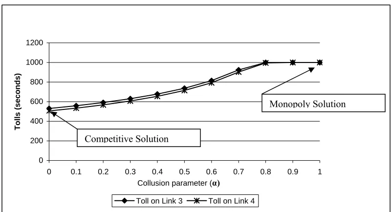
Figure 3 shows, for the case depicted in Scenario 1, how the toll solution moves from Nash Solution when (α= 0) towards the monopoly solution (α= 1) as the level of

collusion is increased. (Note that the graph flattens out beyond α= 0.8 as we have

artificially capped the upper limit of the toll to be 1000 secs.) In particular, when α=1, we obtain exactly the same solution as the monopoly operator’s toll as shown in Table 2.

Figure 3: Tolls for both operators as collusion parameter (α) varies (Scenario 1)

0 200 400 600 800 1000 1200

0 0.1 0.2 0.3 0.4 0.5 0.6 0.7 0.8 0.9 1

T

o

lls (seco

nds)

Toll on Link 3 Toll on Link 4 Collusion parameter (α)

Collusion in Scenario 2

In the case of Scenario 2, where there is an additional route (Link 17) that is not subject to tolls, this form of implicit collusion however does not obtain the solution under monopoly. In particular, consider the situation when α=1, then employing the diagonalisation algorithm, the equilibrium tolls obtained are as shown in Table 5.

Table 5: Tolls and Profits for Scenario 2 considering collusion with α=1

Link Toll (seconds) Revenues (seconds)

Link 7 189.76 116,186

Link 10 186.58 111,216

Total Revenues 227,402

Competitive Solution

Figure 4 illustrates however that the above solution is in fact a local optimum of the total revenue function. The results reported in Table 5 are plotted together in Figure 4 where it is compared against the global optimum which is in fact the solution under monopoly (see Table 2).

Figure 4: Total Revenue Surface as Tolls on Link 7 and Link 10 vary

This illustrates the general difficulty with optimisation algorithms and the potential for local equilibrium to be located. There is also a possibility that in Scenario 2, there continues to be a link (17) available that is in competition with the tolled links and hence even under collusion, there could exist an incentive to capture that untolled traffic by reducing the toll charge which may result in a local solution rather than a global one.

6.

Summary and Conclusions

individual profits non-cooperatively. In particular we recognised that this problem is effectively an Equilibrium Problem with an Equilibrium Constraint and subsequently proposed two heuristics for the solution of this problem. The first is an adaptation of the Gauss-Siedel iterative scheme integrated within an optimisation problem. The second algorithm that we have proposed (SLCP) results from recognising that a Cournot Nash game can be modelled as a complementarity problem and can be solved by sequentially linearising the problem and solving it as a linear complementarity problem. At present we have heuristically employed central differencing techniques to solve this problem, however it is of further research interest to study the use of advances in sensitivity analysis to replace the finite differencing estimation adopted here to further improve the algorithm. Further research would also be directed at efforts in developing new algorithms to solve the EPEC occurring in this situation.

We have also attempted to investigate the possibility of operators colluding implicitly to maximise total profits instead of individual profits. To this effect, we introduced a collusion parameter to reflect the degree of cooperation between operators. Implicit in the assumption was that operators would be willing to reciprocate the action of the other and we have ignored the associated issues of stability of coalitions formed. Nevertheless, even for the simple examples presented in this paper, we have found the potential for multiple equilibria to be obtained. There is much scope to develop this work further considering the case of asymmetric collusion where one operator colludes more than the other which takes us into the area of leader-follower games such as Stackelberg with a subtle difference being that with partial collusion the follower may come out as the winner.

References

[1] Viton P,(1995) “Private Roads”, Journal of Urban Economics, 37(3):260-289.

[2] de Palma, A., Lindsey R, (2000) “Private roads: competition under various ownership regimes”, Annals of Regional Science, 34(1):13-35.

[3] Fisher G, Babbar S, (1996) “Private Financing of Toll Roads” RMC Discussion Paper Series 117, World Bank, Washington DC.

[4] Engel E, Fischer R, Galetovic A, (2002) “A New Approach to Private Roads”,

Regulation, 25(3):18-22

[5] Nash J, (1950) “Equilibrium points in N-person games”, Proceedings of the National Academy of Science, 36(1):48-49.

[6] Pyndyck R, Rubinfeld S, (1992) Microeconomics, Macmillan, New York

[7] Yang H, Feng X, Huang H, (2007) “Private Road Competition and equilibrium with traffic equilibrium constraints”, Manuscript, Hong Kong University of Science and Technology.

[8] Smith M J, (1979) “The existence, uniqueness and stability of traffic equilibria”,

Transportation Resesearch, 13B(4): 295-304.

[9] Dafermos S C, (1980) “Traffic Equilibrium and Variational Inequalities”,

Transportation Science, 14(1):42-54.

[10] Wardrop J G, (1952) “Some theoretical aspects of road traffic research”,

Proceedings of the Institute of Civil Engineers(Transport) Part II, 1(1), 325-378.

[11] Beckmann M, McGuire C B, Winsten C B,(1956) Studies in the Economics of Transportation, Yale University Press, New Haven, Connecticut.

[12] Mordukhovich B S,(2005) “Optimization and equilibrium problems with equilibrium constraints”, Omega-International Journal of Management Science,33(5):379-384.

[13] Su C, (2005) “Equilibrium Problems with Equilibrium Constraints: Stationarities, Algorithms, and Applications”, PhD Thesis, Department of Management Science and Engineering, Stanford University.

[14] Mordukhovich, B S, (2006) Variational Analysis and Generalized Differentiation. II: Applications, Grundlehren Series in Fundamental Principles of Mathematical

[15] Ortega, J M, Rheinboldt C R, (1970) Iterative Solution of Nonlinear Equations in Several Variables, Academic Press, New York.

[16] Judd K, (1998) Numerical Methods in Economics, MIT Press, Cambridge,MA.

[17] Harker P T, (1984) “A variational inequality approach for the determination of Oligopolistic Market Equilibrium”, Mathematical Programming,30(1):105-111.

[18] Cardell J, Hitt C, Hogan W,(1997) Market Power and Strategic Interaction in Electricity Networks, Resource and Energy Economics, 19(1-2):109-137.

[19] Hobbs B F, Metzler C B, Pang J S,(2000) “Strategic Gaming Analysis for Electric Power Networks: an MPEC Approach”, IEEE Transactions on Power Systems,

15(2):638-645.

[20] Lawphongpanich, S Hearn, D W, (2004) “An MPEC Approach to Second-Best Toll Pricing”, Mathematical Programming, 101B(1):33-55.

[21] Pang J S, Chan D,(1982) “Iterative methods for variational and complementarity problems”, Mathematical Programming, 24(1):284-313.

[22] Dafermos S, (1983) “An iterative scheme for variational inequalities”, Mathematical Programming, 26(1):40-47.

[23] Gabay D, Moulin H, (1980) “On the uniqueness and stability of Nash-equilibria in non cooperative games”, In: Bensoussan A, Kleindorfer P, Tapiero C (eds) Applied Stochastic Control in Econometrics and Management Science: Contributions to Economic Analysis, Vol 130, North Holland, Amsterdam: 271-293.

[24] Kolstad C, Matthisen L, (1991) “Computing Cournot-Nash equilibrium”, Operations Research, 39(5):739-448.

[25] Lemke C E, (1965) “Bimatrix Equilibrium Points and Mathematical Programming”,

Management Science,11(7):681-689.

[26] Ferris M, Munson T, (2000) “Complementarity problems in GAMS and the PATH solver”, Journal of Economic Dynamics and Control, 24(2):165-188.

[27] Hooke R, Jeeves T A,(1961) “Direct Search Solution of Numerical and Statistical Problems”, Journal of the Association of Computing Machinery, 8(2):212-229.

[28] Nelder J A, Mead R,(1965) “A Simplex Method for Function Minimization”,

[29] Koh A, Shepherd S P, Sumalee A S (2007) “Second Best Toll and Capacity Optimisation in Networks”, Proceedings of the Universities Transport Studies Group, Harrogate, January.

[30] Verhoef E T, Nijkamp P, Rietveld P, (1996) “Second-Best Congestion Pricing: The Case of an Untolled Alternative”, Journal of Urban Economics, 40(3):279-302.

[31] Luo Z Q, Pang J S, Ralph D,(1996) Mathematical Programs with Equilibrium Constraints, Cambridge University Press, Cambridge, England.

[32] Chen Y, Florian M,(1995) The nonlinear bilevel programming problem: Formulations, regularity and optimality conditions, Optimization,32(3):193-209. [33] Scheel H, Scholtes S,(1995) Mathematical Programs with Equilirbiuyrm Constraints:

stationarity, optimality and sensitivity, Mathematics of Operations Research,25(1):1-22.

Appendix: The Cutting Constraint Algorithm

Mathematical Program with Equilibrium Constraints

In the case of a single operator (operator is a used here generically) who sets tolls and/or capacities to optimise some objective function which could be to maximise social welfare in the case of a local authority or to maximise profit in the case of a private firm. This optimisation problem is effectively an MPEC. The economic paradigm for a generic MPEC is based on the setting of a Stackleberg game where the leader sets his strategic decision variables and the road users on the network follow. In optimising his objective the decision maker has to take into account the responses of the road users whose route choice is given by Wardrop’s Equilibrium Condition. A large amount of development has occurred in this branch of mathematical optimisation [31] which has applications in e.g. mechanics, robotics and transportation analysis. The primary difficulty with the MPEC is that they fail to satisfy certain technical conditions (known as constraint qualifications) at any feasible point [32] - [33]. In recent research [29], we investigated the use of the cutting constraint algorithm (CCA) [20] to solve an MPEC in the context of second best congestion pricing and capacity optimisation.

Reinterpretation of Variational Inequality Condition

Let us define the 2 additional variables

a

β : a pre-specified upper bound on capacities, β =[ ],βa a∈B

τ : a pre-specified upper bound on tolls, τ =[ ],τa a∈B

From convex set theory, e.g. [34]9,

_{( )}

set of extreme points. Hence we can rewrite the equilibrium condition (3) using the following:

(

) (

)

(

) (

)

e E

τ β _{⋅ − −} −1 τ β _{⋅ − ≥ ∀ ∈}

c v u v D d q d

Where ( , )_{u q}e e is the vector of extreme link flow and demand flow indexed by the

superscript e, and E is the set of all extreme points of Ω.

A Cutting Constraint Algorithm for the MPEC

The Cutting Constraint Algorithm redefines the variational inequality using the extreme points as shown above. Together with the initial extreme point, generated by an initial shortest path problem, and the constraints defining feasible flows, the master problem is solved to find the optimal tolls and capacities at each iteration. Subsequently new extreme points (“cuts”) are found by solving a sub problem using the results for the current iteration.

The CCA Algorithm is shown as follows:

Step 0: Initialise the problem by finding the shortest paths for each O-D pair; set l

(iteration counter) = 0; define the aggregated link flow and demand flow

( , )_{u q}l l ; and include _{( , )u q}l l into _E.

Step 1: Set l= +l 1 Solve the Master Problem with all extreme points in E and

obtain the solution vector

₍

₎

(

)

Step 2: Solve the Sub Problem with

(

)

l l _{τ β}l l

v d and obtain the new extreme point

(ul_,ql_);

Step 3: Convergence Check:

If _{c v}

(

) (

)

(

(

)

)

(

)

(

)

Step 1.

The Master Problem in Step 1 is defined as follows:

( ) ( ) ( )

(

) (

)

( ) (

)

min , , ,

. .

0 for given and 0 for given and

,

, , 0 for

a a

a a

T _e T _e

s t

a B

a B

τ β ψ τ β

τ τ ε

β β γ

τ β −

≤ ≤ ∀ ∈ ≤ ≤ ∀ ∈ ∈ Ω ⋅ − − ⋅ − ≥ v d 1 v d v d

c v u v D d q d ∀ ∈e E

The sub problem of Step 2 is a shortest path problem which is formulated as follows:

( ) ( )

(

)

( )

1 ,

min , , , , . .

,

T T

s t

τ β _{⋅ −} − τ β _⋅

∈ Ω

u q c v u D d q

u q