TDR probes for the measurement of root zone soil moisture

University of Southern Queensland

Faculty of Engineering and Surveying

TDR Probes for the

Measurement of Root Zone

Soil Moisture

A Dissertation submitted by

Gary David Bolitho

In partial fulfillment of the requirements of

Course ENG4111 –Research Project Part 1

Course ENG4112 – Research Project Part 2

Thesis for BEngBBus: Batchelor of Engineering – Electrical/Electronic

Batchelor of Business - Leadership

Abstract

There can be no doubt that the efficient management of water resources is a topic that is highly relevant today. A decline in traditional levels of seasonal rain is impacting on rural and urban areas alike as public attention is directed towards recycling programs and public campaigns of efficient use of water. In agriculture, crop yields are directly related to soil moisture, levels that are most important at the root zone area of the plant.

There have been many technical approaches to the monitoring and control of soil moisture levels. One of the most convenient and accurate in-situ methods that has established itself as a recognised standard around the world uses Time Domain Reflectometry (TDR) to determine volumetric water content of the soil.

TDR is most popularly used with soil probes (typically 30 - 60 cm in length) that are inserted directly into the soil and produce a soil moisture measurement that is averaged over the length of the probes. More specific information such as the soil moisture in the root zone is not easily determined with such probes.

Disclaimer

University of Southern Queensland

Faculty of Engineering and Surveying

ENG4111 Research Project Part 1 &

ENG4112 Research Project Part 2

Limitations of Use

The Council of the University of Southern Queensland, its Faculty of Engineering and Surveying, and the staff of the University of Southern Queensland, do not accept any responsibility for the truth, accuracy or completeness of material contained within or associated with this dissertation.

Persons using all or any part of this material do so at their own risk, and not at the risk of the Council of the University of Southern Queensland, its Faculty of Engineering and Surveying or the staff of the University of Southern Queensland.

This dissertation reports an educational exercise and has no purpose or validity beyond this exercise. The sole purpose of the course "Project and Dissertation" is to contribute to the overall education within the student’s chosen degree programme. This document, the associated hardware, software, drawings, and other material set out in the associated appendices should not be used for any other purpose: if they are so used, it is entirely at the risk of the user.

Professor Frank Bullen

Dean

Certification

I certify that the ideas, designs and experimental work, results, analyses, and conclusions set out in this dissertation are entirely my own effort, except where otherwise indicated and acknowledged.

I further certify that the work is original and has not been previously submitted for assessment in any other course or institution, except where specifically stated.

Gary David Bolitho

Student Number: 0019921385

Signature

Acknowledgements

The successful completion of this thesis was brought about with the assistance of many people to whom I am most appreciative.

To my supervisor Dr. Jim Ball for his guidance, supervision and valuable advice. In particular for his understanding and patience with the unexpected interruptions that forced a twelve month delay mid-term.

To my friend Mr. Ian Santinella of San-Tech Machining (14 Rockla Ct. Toowoomba) for his interest and assistance in the construction of probes, supply of materials and use of workshop tools and equipment.

Table of Contents

PAGE

Abstract ...i

Disclaimer... ii

Certification... iii

Acknowledgements ... v

Table of Contents...vi

List of Figures ...ix

List of Tables ... xii

Chapter 1 Introduction...1

1.1 Introduction and Background... 2

1.2 Project Aims and Specific Objectives ... 4

1.3 Conclusions: Chapter 1... 5

Chapter 2 Literature Review ...6

2.1 Introduction ... 7

2.2 Theory of TDR for Soil Moisture Measurement ... 7

2.3 Application of TDR for Soil Moisture Measurement ... 10

2.4 Development of TDR Practices ... 13

2.5 Conclusions: Chapter 2... 21

Chapter 3 TDR Equipment and Laboratory Procedures ...22

3.1 Introduction ... 23

3.2 TDR Equipment - TRASE ... 23

3.3 TDR Equipment – Theory of Operation ... 25

3.4 Soil Preparation ... 29

3.5 Laboratory Test Procedures... 29

3.6 Laboratory Familiarisation Test Results... 31

3.7 Conclusions: Chapter 3... 33

Chapter 4 Transmission Line Considerations for TDR ...34

4.2 Transmission Line Modeling ... 35

4.3 Standard Probe in Air ... 41

4.4 Standard Probe in Water... 44

4.5 Conclusions: Chapter 4... 46

Chapter 5 Prototype Probe Design...48

5.1 Introduction ... 49

5.2 Standard Probe Construction... 49

5.3 Arbitrary Design Requirements... 50

5.4 Transmission Line Considerations ... 52

5.4.1 Transmission Line Modeling ... 52

5.4.2 General Lattice Diagram... 56

5.5 Probe Characteristic Impedance... 57

5.6 Lattice Diagram and TDR Waveform... 60

5.6.1 Prototype Probe in Air ... 60

5.6.2 Prototype Probe in Water... 63

5.7 Mechanical Construction ... 66

5.8 Conclusions: Chapter 5... 68

Chapter 6 Laboratory Procedures and Calibration of Prototype Probe ...69

6.1 Introduction ... 70

6.2 Soil Used for TDR Measurements ... 70

6.3 Laboratory Procedures ... 70

6.4 TRASE Testing Problems ... 78

6.5 Calibration of Prototype Probe in Air and Water ... 80

6.6 Conclusions: Chapter 6... 83

Chapter 7 TDR Soil Measurements and Analysis ...84

7.1 Introduction ... 85

7.2 TDR Measurements in Soil ... 85

7.3 Impedance Mismatch inside First Probe Section ... 94

7.4 Conclusions: Chapter 7... 98

Chapter 8 Simulation Design and Testing...99

8.1 Introduction ... 100

8.2 Drawing Environment ... 101

8.2.1 Preference Setting... 101

8.2.2 Structure Definition ... 102

8.2.3 Discretisation and Drawing Conversion ... 107

8.3 Simulation Environment ... 108

8.3.1 Pre Processing... 108

8.3.2 2D Post Processing ... 111

8.4 Conclusions: Chapter 8... 116

Chapter 9 Conclusions and Recommendations...118

9.1 Introduction ... 119

9.2 Overview of Thesis Work Carried Out ... 119

9.3 Interpretation of Results Achieved ... 122

9.4 Further Research and Recommendations... 122

9.5 Conclusions: Chapter 9... 123

List of References ...124

Bibliography ...127

Appendix A: Project Specifications ...129

Appendix B: Project Timelines ...133

Appendix C: MATLAB Scripts ...136

Appendix D: Probe Details...138

List of Figures

Page

Figure 2.1 Topp System for TDR Measurement of Coaxial Soil Sample ... 10

Figure 2.2 Universal Topp Curve ... 11

Figure 2.3 Universal Topp Curve (Linear Relationship between Volumetric Water Content and Apparent Dielectric Constant) ... 12

Figure 2.4 Examples of TDR Probes in Use ... 14

Figure 2.5 The Shape of Interrogated Soil by TDR Probes ... 16

Figure 2.6 Three-Wire Probe of Zegelin, White & Jenkins (1989)... 17

Figure 2.6 Diode Shorting Probes of Various Lengths... 18

Figure 2.8 TDR probe cross section, showing inner and outer conductor dimensions .... 20

Figure 3.1 TRASE Equipment ... 24

Figure 3.2 TRASE Measurement System showing Capture Window ... 25

Figure 3.3 Details of the TRASE Capture Window – Typical Waveform for Uniform Wet Soil ... 26

Figure 3.4 Graphical Representation of TRASE Inbuilt Lookup Table ... 28

Figure 3.5 TRASE Capture Window during Laboratory Experimentation... 30

Figure 3.6 Results of Laboratory Familiarisation Testing with TRASE Instrument... 31

Figure 3.7 Graph Showing the Difference Between the Actual Water Content and that Measured by the TRASE Instrument for the Sandy Loam Soil ... 32

Figure 4.1 TDR System TX-line Circuit Diagram – 3-Wire Standard Probe ... 36

Figure 4.2 Simple Lattice Diagram for Standard 3-Wire Probe ... 38

Figure 4.3 Concept TDR Waveform... 40

Figure 4.4 Lattice Diagram (Standard Probe in Air) ... 43

Figure 4.5 TDR Waveform (Standard Probe in Air)... 43

Figure 4.6 Lattice Diagram (Standard Probe in Water)... 45

Figure 5.1 Structural Diagrams of Standard Probes (A) 3-Wire and (B) 2-Wire ... 49

Figure 5.2 Concept Structure for 3-wire Prototype Probe ... 51

Figure 5.3 Signal Splitting at Launch Point... 52

Figure 5.4 Direction of Signal Travel at Launch Point ... 53

Figure 5.5 Equivalent Circuit for Initial Launch of Wave ... 53

Figure 5.6 Direction of Signal travel when returning to Launch Point... 55

Figure 5.7 Equivalent Circuit for Wave reflected back off Open Circuit End... 55

Figure 5.8 General Lattice Diagram for Prototype Probe ... 57

Figure 5.9 Lattice Diagram for Prototype Probe in Air (Ka = 1) ... 62

Figure 5.10 TDR Waveform for Prototype Probe in Air (Ka=1) ... 63

Figure 5.11 Lattice Diagram for Prototype Probe in Water (Ka=81) ... 65

Figure 5.12 TDR Waveform for Prototype Probe in Water (Ka=81) ... 65

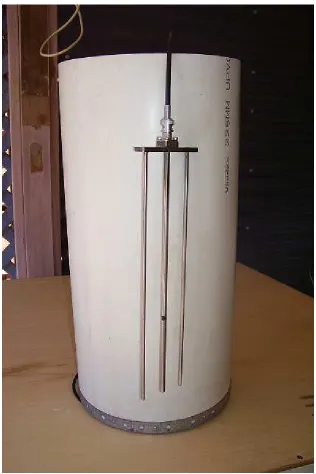
Figure 5.13 Overall Size and Appearance of Prototype Probe ... 67

Figure 5.14 Disassembled View of Prototype Probe ... 67

Figure 5.15 Launch Point Connector of Prototype Probe... 68

Figure 6.1 Laboratory Testing Tube (with Prototype Probe shown)... 71

Figure 6.2 Laboratory Testing Tube (top view) ... 72

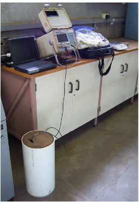
Figure 6.3 Measurement System including TRASE and Soil Testing Tube... 73

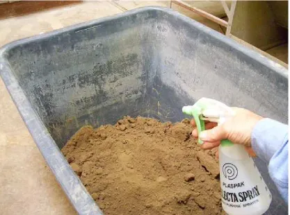
Figure 6.4 Application of Water to Soil Sample in 200litre Tub ... 74

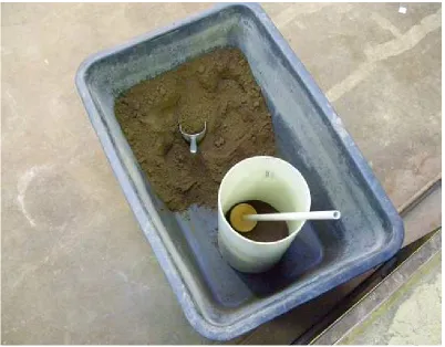
Figure 6.5 Compacting Soil Sample to Ensure Even Density ... 75

Figure 6.6 Downloading of TDR Waveforms to Laptop via RS232 Serial Port ... 76

Figure 6.7 Accurate Weighing of Soil Sample After 24 Hours Drying... 77

Figure 6.8 TDR Waveform of Short-Circuited Coaxial Transmission Line ... 79

Figure 6.9 Prototype Probe TDR Waveform Comparisons (in Air) ... 81

Figure 6.10 Prototype Probe TDR Waveform Comparisons (in Water)... 81

Figure 6.11 Prototype Probe TDR Waveform Comparisons in Water (15-25ns)... 82

Figure 7.1 TDR Waveforms for Prototype Probe (0-50 ns) ... 87

Figure 7.2 TDR Waveforms for Prototype Probe (15-25 ns) ... 88

Figure 7.3 TDR Waveform for Prototype Probe (16% Water) ... 89

Figure 7.5 Comparison of Measured Water Content by Prototype Probe to Actual... 92

Figure 7.6 Investigation of Air Gap on Characteristic Impedance ... 95

Figure 8.1 Empire Draft Environment: Setting of Preferences ... 102

Figure 8.2 Empire Draft Environment: Structure Definition using Layers ... 103

Figure 8.3 Layer List: Creation of Layers for Different Materials... 104

Figure 8.4 Property Editor: Setting Material Properties for Launch Point Connector . 105 Figure 8.5 Library Element Editor: Coaxial Port Properties... 106

Figure 8.6 Field Storage Area: Transparent View ... 107

Figure 8.7 Boundary Conditions: Set to be Perfectly Matched (Absorbing) ... 109

Figure 8.8 Excitation Defined: Fast Rise-Time Pulse ... 110

Figure 8.9 Simulation End Criterion: Number of Steps and Energy Decay Checksum . 111 Figure 8.10 2D Graph Selection and Setup ... 112

Figure 8.11 2D Graph: Time Domain Voltage Waveform for Probes... 113

Figure 8.12 3D Simulation: Field Animation Controls ... 114

Figure 8.13 3D Simulation Snapshot: Propagation of Electromagnetic Fields ... 115

Figure 8.12 3D Simulation: Effective Length of Probe is Longer ... 116

Figure B.1 Proposed Timetable of Major Project Activities 2006 ... 134

Figure B.2 Amended Project Timeline for S2 2007 (2nd part of Project Delayed by 12 Months) ... 135

Figure D.1 Prototype Probe with 50Ω Coaxial Connection Lead ... 139

Figure D.2 Details of Launch Point Connector Assembly... 139

Figure D.3 Stainless Steel Arbour Showing Connection Details for Coaxial BNC Socket ... 140

Figure D.4 Panel Mount BNC Coaxial Socket with RG58U Cable ... 140

Figure D.5 Engineering Drawings of Prototype Probe ... 141

List of Tables

Table 1.1 Dielectric constants of soil constituents and major textures of soils... 4

Table 5.1 Design Variations of Prototype Probe... 59

Table E.1 Measurement Results for All Probes ... 144

1.1 Introduction and Background

There have been several approaches to the monitoring and control of soil moisture in recent years. Industries that cover aspects of hydrology, agriculture, engineering and forestry have looked for fast, economical, and accurate methods that promote economical and good management practice of water as a limited resource.

Traditionally, soil water content was obtained through gravimetric testing procedures that required soil samples from the field to be weighed and then oven-dried. The change in mass is then used to accurately calculate the volumetric water content of the soil. This of course is a time-consuming and expensive procedure that not only has environmental implications associated with the removal of soil from the environment, but also represents significant tendency for error. Errors can be experienced due to poor sampling procedures including deficient selection of soil samples that may not be representative of the area of interest. In-situ testing has become the favored approach.

Early in-situ testing was accomplished through the use of the neutron probe and the dual gamma ray techniques (Greacen 1981). Both of these methods overcame the destructive nature of previous laboratory sampling and provided a quick and accurate method of soil moisture measurements. Disadvantages however are the dangerous radioactive nature of the technology. Also the neutron probe responds to the hydrogen content of the soil itself and not just that of the water present in the soil. This means that calibration of the instrument is difficult as it must first account for the type of soil present. Use of these technologies is also restricted by government laws. To overcome these limitations, work in the nineteen-eighties by researchers focused on the dielectric properties of the soil as a means of calculating water content.

to soil moisture content. One early technique developed relied on the capacitive effect of the water present in the soil (Dean, Bell & Batty, 1987).

Testing bulk soil dielectric permittivity with capacitance probes inserted into the soil is a quick and convenient method. The equipment necessary is inexpensive and has none of the dangerous radioactive components of the earlier technologies. Results from capacitance techniques (Selig & Mansukhani, 1975; McKim. et al., 1980) however are greatly dependant on specific electrode configurations and detailed calibration in the field. Limitations arise with the variation in permittivity readings due to the presence of any air gaps between the probe and the soil. The method of installing the probes requires that a suitable tunnel be formed in the ground into which the probes can be inserted. This procedure inherently introduces air gaps. It was also found that the soil type significantly influenced the consistency of results, in particular the conductive properties of the soil. These limitations were largely overcome with research into TDR as an alternative method.

TDR was found to possess all of the advantages of the capacitance probes, but produced more consistent and reliable results (Topp, Davis & Annan, 1980). The technology works by applying an electric pulse to probes inserted into the earth. The probes act as a ‘waveguide’ for this electromagnetic wave as it travels through the soil. The soil is the dielectric material contained by the waveguides. Soil moisture is determined by first measuring the propagation velocity of this electromagnetic wave as it travels along the probes and is reflected off the open end and back to the start of the probes.

constitute the soil. This can be seen with comparison of the typical dielectric constants of these materials:

Table 1.1 Dielectric constants of soil constituents and major textures of soils

Material Dielectric Constant

Air 1

Water 81 @ 20°C

Ice 3 @ 5°C

Basalt 12

Granite 7 - 9

Sandstone 9 - 11

Dry Loam 3.5

Dry Sand 2.5

(Source: Noborio2001, p. 217)

Therefore, TDR makes use of the propagation velocity to calculate the apparent permittivity of the soil. Extensive empirical studies (Topp, Davis & Annan, 1980) enabled a direct correlation of the apparent dielectric permittivity to the soil moisture content (θv). A universal curve that describes this relationship for a particular soil type has been dubbed the Topp Curve. The accuracy of TDR has gained recognition as a world-wide standard to which all other methods are compared.

1.2 Project Aims and Specific Objectives

Laboratory experimentation with soil samples and the university’s TDR equipment is first carried out using the conventional probes provided. A thorough literature review of relevant theory and history of TDR for the use of soil moisture monitoring is also undertaken. This is done to gain an understanding of the current theory and application of TDR in the soil moisture measurement context.

The USQ owns a TDR instrument that is available for the purpose of this project. Familiarisation with the TDR equipment and the theory of TDR is essential for the successful completion of this project. Also is an understanding of the physical properties of soil, the combination of soil and water, soil type and mineral content, all in the presence of a traveling electromagnetic wave.

Specific objectives are then to:

• Design and construct a soil probe that yields soil profile information rather than averaged information.

• Gain familiararity with simulation software; used to aid in the design and testing of potential probe configurations.

• Assess the new probe for accuracy and functionality. The full project specification can be found in Appendix A

1.3 Conclusions: Chapter 1

2.1 Introduction

This chapter will review literature related to the history of soil moisture measurement methods using TDR. This will establish an understanding of the theory of TDR, applications and limitations of its use for soil moisture measurement and developments to date that assist the design of a probe suitable for soil profile determination.

2.2 Theory of TDR for Soil Moisture Measurement

Some of the early work of the application of TDR to determine the dielectric properties of soil was done by Hoekstra & Delaney (1974). They were able to identify that over a range of frequencies the relationship between volumetric water content and the complex dielectric constant is relatively independent of soil type. Leading on from there, much of the work to realise the practical potential of TDR for accurate measurement of soil water content was pioneered by Topp, Davis & Annan, (1980). It was their finding that in the frequency range 1MHz to 1GHz, that the real part of the complex dielectric permittivity of soils (ε') was sensitive to the volumetric water content of the soil. They determined that the relationship was not strong with other physical properties such as soil density and type. In particular, they determined that ε'

was not strongly dependant on frequency as had been the focus of all previous research of TDR for soil moisture measurements.

The focus for Topp, Davis and Annan (1980) was therefore to measure the propagation velocity of a fast rise time pulse through the soil, use this information to first calculate the apparent permittivity (K ) of the soil, and from there to determine an accurate _a

In any given dielectric material, the propagation velocity of an electromagnetic wave (Vp) is less than that of its propagation in free space (c 3 10 m/s

8

×

= ) according to:

r r p c V µ ε

= …………...……… (2.1)

where µr is the dielectric permeability of the soil, and r

ε is the complex permittivity of the soil given by:

      + − = 0 '' ' ωε σ ε ε ε dc

r j ………...……… (2.2)

and σ_dcis the DC conductivity of the dielectric 0

ε is the permittivity of free space (8.854×10−12F /m)

ωis the radian frequency

The magnetic property of nearly all soils does not vary significantly from that of free space so it can be assumed that µr =1

The velocity equation is now reduced to:

r p

c V

ε

Substituting for ε_rwe get:

(

)

1 2 1 2 ' tan 1 1

2 

    + + = δ ε c

V_p ………... (2.4)

where _'

'' tan ε ωε σ ε

δ 

    + = o dc ………...……… (2.5)

Since the propagation velocity is not entirely independent of ε'' the measured dielectric permittivity is generally termed the apparent dielectric permittivity and is given the symbolK_a. Hence the propagation velocity is related to the apparent dielectric permittivity by the simplified equation:

a p

K c

V = ………...… (2.6)

For the soil probes of length L and transit time ( t∆ ) for the pulse to travel the length of the probes from the start to the end and back to the start:

t L Vp

∆

=2 ………….……….. (2.7)

By substitution and rearrangement of (2.6) and (2.7) the apparent dielectric permittivity is related to the propagation velocity by:

2

2 

   ∆ × = L c t

2.3 Application of TDR for Soil Moisture Measurement

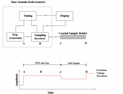
Having been able to calculate the apparent dielectric permittivity from the transit time, Topp, Davis and Annan (1980) then embarked on exhaustive laboratory testing of soil samples in a coaxial cell. They were able to use a standard TDR instrument whose primary use was to find faults in cables. The equipment they used is represented in Figure 2.1.

Figure 2.1 Topp System for TDR Measurement of Coaxial Soil Sample

the remainder is transmitted through the soil sample to the end point D. An open circuit at the end causes the entire signal to be reflected back through the soil sample.

Using the coaxial transmission line cell system, Topp, Davis and Annan (1980a) were able to test different soil types with varying water contents for their transit time and subsequently calculate apparent dielectric permittivity. Through this empirical analysis they were able to derive a 3rd order polynomial that provided accurate representation across the range of soil water contents of general interest. This relationship has since been recognised as a global standard by which all soil water content measurements using TDR methods are now compared. The polynomial was dubbed the ‘Topp Curve’ is shown in Figure 2.2, and is mathematically expressed as:

3 2

7 . 76 0

. 146 3

. 9 03 .

3 v v v

a

K = + θ + θ − θ ………...………. (2.9)

where θ_vis the volumetric water content of the soil.

The Topp Curve when plotted with square root of K against volumetric water content _a

reveals an almost linear relationship as shown if Figure 2.3.

Figure 2.3 Universal Topp Curve (Linear Relationship between Volumetric Water Content and Apparent

Dielectric Constant)

The apparent linear relationship shown in Figure 2.3 is useful for establishing whether the TDR response does in fact provide an average soil moisture reading over the length of the probe. This will now be investigated.

Let the distance from the start of the probe to the end be a measure of distance z. Making use of equation (2.3) it can be said that the time delay taken for the TDR signal to travel the length of the probe (L) is:

∫

∫

=

L r L

p

d dz

c V

dz

0 0

2

2 ε

τ ... (2.10)

c K L V L a p d 2 2 = = τ ... (2.11)

Equating (2.10) and (2.11) gives:

∫

∫

Using the linear relationship of Figure 2.3, and adopting the constant C for the slope of the graph, and Y intercept =2, it can be said that:

v

a C

K =2+ θ ... (2.13)

Equating (2.12) and (2.13) and allowingK_a =ε_r:

( )

[

]

( )

( )

∫

∫

∫

Therefore it can be seen that volumetric water content is indeed found as an average over the length of the probes.

2.4 Development of TDR Practices

TDR could be used to accurately identify wetting fronts within the soil, but this often required intuitive and expert interpretation of the measured reflection signals. Also, it did not necessarily equate to information about a particular profile of interest.

A number of different designs of probes have emerged. Figure 2.4 shows some two and three-wire probes and a coaxial probe.

Figure 2.4 Examples of TDR Probes in Use

The probes in Figure 2.4 have different characteristics and will be described separately. From left to right, they are:

•A twin-wire probe: wires of varying lengths can be connected to the head section, this is the ‘connector’ probe developed by Soil Moisture Equipment Corp™, and is the probe that will be used as a standard during laboratory testing for this thesis.

•Twin-wire probe: developed by Imko Gmbh™. Twin wire probes are most commonly used in the field because of ease of insertion into the soil.

•Three-wire ‘buriable’ probe: developed by Soil Moisture Equipment Corp™ with sealed connections such that the probe can be buried underground.

•Coaxial probe by LTHE (Laboratoire d'étude des Transferts en Hydrologie et

Environnement).

Figure 2.5 The Shape of Interrogated Soil by TDR Probes

(Source: Laurent 1998, p.4)

The second probe in Figure 2.5 is that of a particular type of twin-wire probe that can be placed at different depths in an access tube, recently developed by Imko Gmbh™ (Laurent 1998). The fourth is that of the coaxial cell by LTHE which are preferred for experiments in the laboratory of for calibration (Laurent 1998). With such probes, the measured volume is perfectly defined: this is the whole inner space of the wave-guide. Also compared to the two-wire probes, it can be seen that the three-wire probe provides better definition of the soil volume under investigation. This will be seen to be significant in design considerations that follow.

undesirable signal and information loss at the interface between the two. This was originally overcome with the introduction of a balancing transformer, or balun.

The balun itself however was found to introduce unwanted noise causing difficulties in the signal analysis (Zegelin, White & Jenkins, 1989). To overcome the need for a balun, they undertook to re-design the existing two-wire probes with 3 and 4 wire models for field use. Figure 2.6 shows the 3-wire probe of Zeglin, White and Jenkins (1989). Their analysis of the electric field distribution around the probes closely emulated the results achieved by Topp’s laboratory testing of a coaxial transmission line cell. The new design also minimised the impedance mismatch which occurred with the two-wire probes.

Figure 2.6 Three-Wire Probe of Zegelin, White & Jenkins (1989)

One modern TDR probe in use makes use of a twin wire transmission line with shorting diodes placed between the wires at different intervals along the probe length (Figure 2.7). With electronic control, different combinations of diodes are switched such that the probe is interrogated over the different segments (Hook et al., 1992). Although this provides profiling information, it is considered that spatial resolution of this system is relatively weak (Laurent, 1998).

Figure 2.6 Diode Shorting Probes of Various Lengths

(Source: Moisture Point 2007, p.2)

investigated the accuracy of TDR in different soil types and found that the response of TDR probes is especially sensitive to the region immediately surrounding the probe wires. Since the area between the probes is filled with the switching diodes and a poured epoxy resin, then the dielectric properties of the soil itself is not the region of greatest interrogation by the TDR induced fields.

Recent studies by Laurent (1998) have sought to extract water-content profile information from the TDR measured waveform, in addition to the traditional overall propagation time and corresponding average water content. A TDR signal inversion method called “TDR_SSI” considers the waveform as a set of elementary reflected signals, not only at the beginning and end of the probe, but also every time an impedance discontinuity is encountered in the soil medium. Any variations in water content throughout the sampled soil will lead to fluctuations of the electrical permittivity, and thus of the impedance. These create reflections that combine as an image of the impedance along the probe. Laurent did however identify several limitations to the method. Practical limitations exist with the insertion of the long plastic tubes or rods into heterogeneous type soils. This long length also introduces unwanted signal attenuation in highly conductive soil types causing inaccuracy in calculations. Also identified was some scattering or variation of

a

K with the frequency due to a distribution of relaxation properties throughout the soil.

Figure 2.8 TDR probe cross section, showing inner and outer conductor dimensions 2 conductors outer of number where ln 1 ln 2 1 0 0 0 0 = =               +       = n n a s n a s Z i probe ε µ

π ...……….… (2.15)

2.5 Conclusions: Chapter 2

This chapter has conducted a review of literature to investigate TDR principles and applications of TDR to soil moisture measurement. Firstly the theory of TDR in general was established and mathematical equations derived to support that theory. Secondly the application of TDR was examined; facilitated by an investigation of various methods that have been used and the assortment of probes that have been designed.

3.1 Introduction

This chapter will provided an introduction to the TDR test equipment and its use in the laboratory. Details of the TRASE TDR system will be investigated to gain familiarity with its functions and its ability to determine transit time of the signal energy through a soil sample such that apparent dielectric constant can be calculated. It will be shown how the transit time is used to determine volumetric soil moisture content. Soil preparation and laboratory testing procedures will be established, followed by familiarisation testing of soil samples using the TRASE system. Evaluation of the laboratory results provides a benchmark for the rigorous testing that will be required once the prototype probes are designed and constructed.

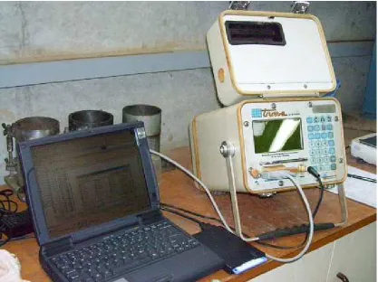
3.2 TDR Equipment - TRASE

Figure 3.1 TRASE Equipment

3.3 TDR Equipment – Theory of Operation

General principles of operation of TDR measurement equipment was presented in the literature review chapter (refer to section 2.3: Application of TDR for Soil Moisture Measurement). Figure 3.2 shows how the TRASE TDR system works.

Figure 3.2 TRASE Measurement System showing Capture Window

The TDR processor generates a series of fast rise time microwave pulses (rise time < 200ps) which propagate down the transmission line that consists of the coaxial cable and the waveguides that are inserted into the soil. The start of each pulse is referred to as the incident pulse and is the point from which subsequent time measurements are made during the automatic determination of moisture content. It is through a series of pulses and time-shifted measurements that the TRASE system builds up an accurate picture of the TDR response. The iterative process will now be described.

10ps. Each measurement point is stored such that the complete time range of interest is covered. In addition, after the complete time span is covered, the same process is repeated a number of times to provide an ‘average’ value for each of the 1000 points. Not all of the 1000 points are used for graphical display. How the stored data is processed by the TRASE system software for graphical display will be discussed next.

The TRASE system software detects the point at which the TDR pulse reaches the start of the probe. The time from the start of the pulse measuring process to the time of the start of the probes is called the ‘zero-set’ time. The time of the first reflection off the end of the probes is also detected. It can be seen from Figure 3.2 that the difference between these two times is determined as the transit time. The TRASE system software will then allocate a portion of the collected waveform that contains these two points to be displayed as the ‘capture window’. Figure 3.3 shows detail of a typical waveform displayed in the instrument’s capture window after conducting a test in moist soil.

Figure 3.3 Details of the TRASE Capture Window – Typical Waveform for Uniform Wet Soil

(∆t =t₂ −t₁) so that the apparent dielectric permittivity K can be calculated. _a

Determination of the point of first reflection is achieved through a process of tangent fitting. In Figure 3.3 it can be seen that the first tangent is fitted to the section of graph as the wave travels along the probe; the second tangent is fitted to the section of graph immediately following the reflection. It is the intersection of these two tangents that is determined as the reflection point.

Having determined apparent dielectric permittivityK , the TRASE then converts this to a a measure of volumetric water content via an inbuilt look-up table. The user can define certain look-up table parameters or select to use the standard tables calibrated using the universal Topp equation. The Topp equation is only valid for up a range of about 0-40% volumetric water content. The TRASE lookup table however has been extended to cover 0-100% range, based on testing carried out by the manufacturer SoilMoisture Corp. For

the purpose of this thesis it is still only the range 0-40% that is useful since at about 30% most soils become saturated. The TRASE inbuilt lookup table is displayed in graphical form in Figure 3.4 below. It can be observed from the graph that there is a relatively linear relationship between apparent dielectric constant and volumetric water content over the full range of 0-100%. Taking an example, if a reading of K =56 is measured, _a

the corresponding volumetric water content (θv) would be read as 78%. For a reading of a

K =18 is measured, the correspondingθ_vwould be read as 30%. The variation of K is _a

.F

ig

u

re

3

.4

G

ra

p

h

ic

a

l

R

e

p

re

se

n

ta

ti

o

n

o

f

T

R

A

S

E

I

n

b

u

il

t

L

o

o

ku

p

T

a

b

3.4 Soil Preparation

To gain familiarity with the TRASE equipment it was decided to test various soil samples in the laboratory. In alignment with the coaxial cell testing done by Topp, Davis and Annan (1980) and Habash (1994), a sandy loam type soil sample was selected and tested under various water content conditions. Distilled water, rather than town supply or rain water was chosen to also be consistent with established laboratory testing procedures. The process used will now be described.

First the soil sample was sieved to 10mm to remove large stones. The soil was then oven dried for 24 hours at105oC to remove all water content and weighed. The dried soil was placed in a plastic tube of sufficient size to allow at least 5 cm of soil to be present around the outermost dimensions of the probes and beneath the probes. This requirement would ensure adequate containment of the electromagnetic wave through the soil under test, without any of it being exposed to the air outside the bucket or floor underneath. This requirement is also in keeping with proven laboratory procedures used in previous experimentation (Habash, 1994).

3.5 Laboratory Test Procedures

Standard ‘connector’ type probes of 30cm length were arbitrarily chosen to use in the initial soil testing procedures. The TDR probes were place in the soil up to the full depth of the probes for each test. Five concurrent measurements were made in each of three probe positions in the bucket for every test. Apparent dielectric content and volumetric water content were recorded with an average for the test being calculated.

filled so that gravimetric testing could be carried out to test against the volumetric data being collected. The test procedure could be summarised in six distinct steps:

1. Oven dry soil sample at 105oC for 24 hours.

2. Determine the amount of water required to produce specific water content level. 3. Add and mix measured quantity of water with soil.

4. Leave soil sample to cure for 24 hours

5. Use the TRASE instrument to gather measurements in three different probe positions

6. Take an oven dried soil sample to verify the water content.

Please note that for these initial familiarisation tests, Step 4 was omitted for expediency purposes. This step will however be a part of any formal laboratory testing procedures to verify the operation of the new prototype probe yet to be made.

Figure 3.5 below shows a photo of the TRASE front panel and a typical TDR waveform measured during laboratory experimentation. The first vertical line on the left is the determined zero-set point, and the other two vertical lines are adjustable by the user such that transit time calculations can be made on screen.

3.6 Laboratory Familiarisation Test Results

Results of the familiarisation testing showed good alignment with the measurements of others (Habash 1994, Topp, Davis & Annan, 1980) and are shown in Figure 3.6.

Comparison of Measured Dielectric Characteristics With Topp's Universal Curve

0 5 10 15 20 25

0% 5% 10% 15% 20% 25% 30% 35%

Volumetric Water Content

A

p

p

a

re

n

t

D

ie

le

c

tr

ic

P

e

rm

it

ti

v

it

y

K

a Measured Curve_{Poly. (Topp Curve)}

Poly. (Measured Curve)

Figure 3.6 Results of Laboratory Familiarisation Testing with TRASE Instrument

Comparison Between Actual and Measured Water Content

y = 1.2229x + 0.003 R2 = 0.8294

0% 5% 10% 15% 20% 25% 30% 35% 40%

0% 5% 10% 15% 20% 25% 30% 35%

Gravimetric Water Content

T R A S E M e a s u re d W a te r C o n te n t

Figure 3.7 Graph Showing the Difference Between the Actual Water Content and that Measured by the

TRASE Instrument for the Sandy Loam Soil

3.7 Conclusions: Chapter 3

4.1 Introduction

The design of soil probes for use with TDR necessitates an understanding of transmission line characteristics to enable interpretation of the signal produced. This chapter will first develop a transmission line model for a lossless TDR system. Next, an investigation of the waveform as it passes through the system will be facilitated by the use of lattice diagrams. Practical examples of standard probes in air and in water will reveal the effect of probe design and material permittivity on TDR waveforms. In particular it is the effect of the impedance mismatch that the signal encounters at the junction of the coaxial transmission line and the start of the probe that will be investigated. Relative timing and reflection characteristics are examined.

4.2 Transmission Line Modeling

One of the simplest modeling tools available to understand the time domain response of a short transmission line is the lattice diagram. The lattice diagram keeps track of multiple reflections and is usually based on the assumption of lossless line characteristics. On a lossy transmission line it is the high frequency components of a pulse spectrum that define the leading and trailing edges, so that a pulse on a lossy line becomes progressively more rounded as it travels. On a lossless line however, the amplitude and waveshape of the pulse is maintained, so that the line behaves purely as a time delay.

The TDR system can now be represented by consideration of the various components and how they relate to transmission line properties. The components of interest are the step generator, the coaxial transmission line of impedanceZ , and the probe section that 0 represents an open circuit transmission line with impedanceZ_pSoil. The impedance Z_pSoil

will vary according to the dielectric properties that the soil and moisture present. Figure 4.1 shows the TDR transmission line circuit with standard 3-wire probe.

Figure 4.1 TDR System TX-line Circuit Diagram – 3-Wire Standard Probe

however some will be reflected and travel back down the probe again. This process will continue until the energy in the reflected pulse decays to zero.

The extent to which the incident energy is reflected off the mismatch will depend on the reflection coefficient of the mismatch and is given the symbol ρ, where:

0 0

Z Z

Z Z

pSoil pSoil

+ − =

ρ ... (4.1)

If the step value that first appears is considered to be normalized with a value 1, then the amount that propagates through the mismatch is determined as the transmission coefficient (t), such that:

(

)

0 2 1

Z Z

Z t

pSoil pSoil

+ =

+

= ρ

...…….………...………. (4.2)

The time taken for the pulse to travel from the start of the probe to the end, and reflected back to the start of the probe again is the time delay (T). Making use of equation (2.8) from earlier, we can say:

c K L

T = 2 a ……….……….. (4.3)

Using the lattice diagram of Figure 4.2 and following the path of the pulse for the first three reflections, it is possible to derive a Laplace Transform that expresses the resultant waveform.

(

)

(

)

(

)

(

)

(

)

... 1 1 1 1 2 sT sT sT sT g

meas t e t e t e e

V

V = + ρ+ −ρ − − −ρ ρ − + −ρ ρ − + − …. (4.4)

Equation (4.4) needs some clarification:

• The exponential terms are used to describe each time delay

• T1 is introduced to account for the measurement of the voltage as it occurs at the output of the step generator and is time displaced from the probes by the distance required to travel along the length of the coaxial transmission line. An equation to express this relationship for T1:

c L

T1 = 2 coax εrCoax ………...….………...…… (4.5) where εrCoax is the dielectric permittivity of the coaxial cable.

• The initial voltage that appears on the transmission system will only be half of the generated voltage due to the fact that the output impedance of the step generator is matched to the characteristic impedance of the coaxial transmission line

(

)

Combining the mathematical relationships with the lattice diagram methodology, a graphical representation can be derived, shown in Figure 4.3.

Figure 4.3 Concept TDR Waveform

In the next section, the time domain response of a standard 3-wire probe of length 10cm

(

)

(

)

4.3 Standard Probe in Air

At this stage it will be beneficial also to calculate the impedance of the probe itself and equation (2.15) derived by Ball (2002) and presented earlier in chapter 2 will be used:

              +       = n a s n a s Z i probe 0 0 0 0 ln 1 ln 2 1 ε µ

π …………...……….… (4.7)

conductor inner of radius conductor outer of radius separation s conductors outer of number where = = = = i o a a n

For permeability and permittivity constants

m F m H / 10 85 . 8 / 10 26 . 1 12 0 6 0 − − × = × = ε µ

The equation is reduced to:

              +       ≈ 0 0 2 ln 2 1 ln 60 a s a s Z i

probe …………...………...……. (4.8)

For the 3-wire probe, there are two outer conductors (n=2), equal wire size (a_o =a_i =3mm) and with equal separation (s=25mm). Substituting these values into equation (4.8), the impedance of the probe will be:

Ω =             × +       =               +       = 03 . 170 03 . 0 2 25 . 0 ln 2 1 03 . 0 25 . 0 ln 60 2 ln 2 1 ln 60 0 0 a s a s Z i probe ... (4.9)

In air Ka =εr =1, therefore:

The difference between the impedances of the probe and the coaxial line will create a mismatch at the interface of the two such that the reflection coefficient will be: 546 . 0 0 0 = + − = Z Z Z Z pSoil pSoil ρ ... (4.11)

Also, the transmission coefficient at the mismatch is calculated as:

546 . 1 1 = + = ρ t ………...……….. (4.12)

Time delays along the length of the coaxial cable (T1) and along the probe are:

ns T 21 10 3 16 . 2 2 . 2 2 8 1 = × ×

= _{………...……….. (4.13)}

ns T 7 . 0 10 3 1 1 . 0 2 8 = × ×

= _{………. (4.14)}

If generator step voltage is assumed to be 2V then: V 1 2 2 2 0

0 = = =

+ = g g g initial V Z Z Z V

With the values now calculated, the lattice diagram can be constructed and waveform produced, shown in Figures 4.4 and Figure 4.5 respectively.

Figure 4.4 Lattice Diagram (Standard Probe in Air)

4.4 Standard Probe in Water

All previous calculated attributes will be the same as in the previous scenario, except for the effect of the water permittivity on probe impedance. For water, it will be assumed relative permittivity εr =Ka =81, therefore effective probe impedance will be:

Ω = = 9 . 18 0 a probe pSoil K Z Z ... (4.16)

The variation of impedances of the probe and the coax will create a mismatch at the interface of the two such that the reflection coefficient will be:

452 . 0 0 0 − + − = Z Z Z Z pSoil pSoil ρ ... (4.17)

Also, the transmission coefficient at the mismatch is calculated as:

548 . 0 1 = + = ρ t ………...……….. (4.18)

Time delays along the length of the probe will be:

ns T 6 10 3 81 1 . 0 2 8 = × ×

= _{………. (4.19)}

Figure 4.6 Lattice Diagram (Standard Probe in Water)

Figure 4.7 TDR Waveform (Standard Probe in Water)

understanding of the basic nature of signal response, since in a real application, the entire transmission line system is subject to frequency dependent losses. It is the high frequency components of the fast rise time pulse that are most affected by losses during transmission. Other losses are caused by the DC conductivity of the soil (due to the presence of minerals, salts, etc.) and also by the dielectric polarisation losses of the various soil constituents, especially the water. In general, the effect of losses will contribute significantly to rounding of square edges within the waveform, signal attenuation and final DC values.

One of the important features to note in the two previous TDR waveforms is that the amplitude of each subsequent reflection decreases, with the final voltage approaching that of the generator output voltage (V ). This is intuitive of DC considerations for an open g circuit; that is the transmission line is terminated in an open-circuit. As expected then, after only a few reflections the step generator eventually sees an open circuit and thus voltage measured at the sampling receiver Vmeas =Vg. Also of importance is the effect that the relative permittivity characteristics of water and air have on the impedance characteristics of the probe and subsequent waveforms. The first implication is for the creation of an impedance mismatch that affects the reflection properties of the transmission line when the incoming signal encounters the mismatch. Secondly is the effect on timing of reflections. The transit times for reflections are seen to increase with the relative permittivity of the medium surrounding the probe. In this case the transit time increased from 0.7ns for air (Ka=1) to 6ns for water (Ka=81). The next section will investigate these properties when the signal is injected at a point along the length of the probes rather than at the probe’s head.

4.5 Conclusions: Chapter 4

5.1 Introduction

Probe design requirements will be investigated in this chapter such that an effective prototype probe can be constructed. Arbitrary requirements determine overall size and shape while transmission line considerations reveal information about the expected behaviour of an incident signal that is launched from a position two thirds the distance along the probe’s centre conductor. Lattice diagrams are again used to determine this behaviour. Workshop production of the designed prototype probe is then detailed.

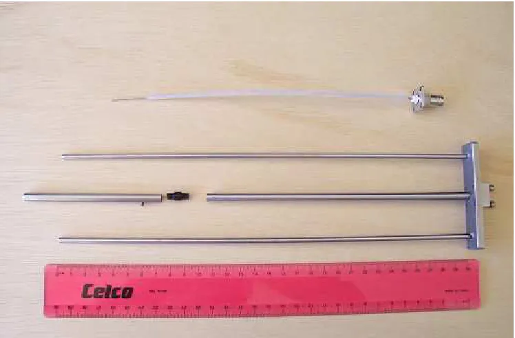
5.2 Standard Probe Construction

Conventional 3-wire and 2-wire probes in use are represented in Figure 5.1

Figure 5.1 Structural Diagrams of Standard Probes (A) 3-Wire and (B) 2-Wire

The three-wire probe is a good approximation of a coaxial cell (Zeglin, White & Jenkins 1989) and does not need an impedance matching transformer as does the two-wire. For this reason it was decided to design a prototype based on the 3-wire concept. Of particular notice in Figure 5.1 is the point of signal injection at the top of the centre wire. The centre wire is electrically isolated from the rest of the structure. The probes are pushed full length into the soil.

5.3 Arbitrary Design Requirements

Figure 5.2 Concept Structure for 3-wire Prototype Probe

sizes and separation dimensions? The next section will investigate design implications for characteristic impedance.

5.4 Transmission Line Considerations

5.4.1 Transmission Line Modeling

Transmission line theory can be utilised to analyse the connection of a single 50Ω coaxial transmission line to a parallel 3-wire transmission line. Figure 5.3 gives a representation of the direction of waves at the emergence from the launch point and at the end of the probes.

Figure 5.3 Signal Splitting at Launch Point

investigate the behaviour of the wave at this point. Figure 5.4 shows the direction of signal travel at the launch point while Figure 5.5 displays an equivalent circuit diagram.

Figure 5.4 Direction of Signal Travel at Launch Point

Figure 5.5 Equivalent Circuit for Initial Launch of Wave

than the wave traveling through the soil to the end of the probe. For this reason, the upward traveling wave can be ignored since any reflections will not be seen until much later. It is the downward traveling wave that is of importance and will be tracked.

The voltage reflection coefficient of the incident wave off the mismatch shown in Figure 5.4 will be labeled ρ₁ and can be determined as:

(

)

(

)

For each of the two waves the transmission coefficient will be: )

1

( 1

1 = +ρ

t ... (5.2)

Figure 5.6 Direction of Signal travel when returning to Launch Point

Figure 5.7 Equivalent Circuit for Wave reflected back off Open Circuit End

(

)

(

)

The new transmission coefficient will be: )

1

( ₂

2 = +ρ

t ... (5.4) where 1 represents the first reflected wave t1 =(1+ρ1), thus:

(

) (

)

2 = t +ρ = 1+ρ +ρ

t ... (5.5)

The effect of the two connected transmission lines on the amount of signal transmitted into the coaxial line back towards the TRASE unit can be given as:

       

+ZpSoil

Z Z t

0 0

2 ... (5.6) This will not be the same for the amount of signal transmitted back up the soil to the surface; this will in fact be equivalent to:

        + 0 2 Z Z Z t pSoil pSoil ... (5.7)

5.4.2 General Lattice Diagram

Figure 5.8 General Lattice Diagram for Prototype Probe

5.5 Probe Characteristic Impedance

The probe will be required to give good signal transfer from the coaxial transmission line under a range of various conditions; that is relative permittivity will vary according to the amount of moisture present in the soil. Maximum signal transfer will occur if the impedance mismatch at the launch point is minimised such that:

Ω =

≅ // 50

0 ZpSoil ZpSoil

Z ... (5.8)

Therefore it is desirable that ZpSoil ≅100Ω.

r pSoil probe r probe pSoil Z Z Z Z ε ε = = 0 0 ... (5.9)

In dry soil, apparent dielectric permittivity may be as low as K_a =2. Substitution of r

a

K =2 for ε into (5.9) gives:

Ω = × = = 141 2 100 0probe ZpSoil Ka

Z

... (5.10)

The extreme of the range would be experienced in a situation where soil is saturated. Using the Topp Equation (2.9) and knowledge of soil properties that determine saturation at around 30%, Ka can be calculated as 16.5. In this case:

Ω = × = = 406 5 . 16 100 0probe ZpSoil Ka

Z

... (5.11)

Following on from the above it is desirable then that the characteristic impedance of the probe be somewhere in the middle of the range, say200−250Ω.

Investigations of some variations of wire separation and diameter will determine their effect on characteristic impedance. The earlier equation (4.7) by Ball (2002) will be used for the calculation.

Recalling that: conductors outer of number conductors outer and inner between distance separation conductors outer of radius conductor inner of radius 0 = = = = n s a a_i

chapter. In general it was decided to design a probe of similar dimensions to the commercially available ones. A further consideration was that the hollow centre conductor must have sufficient internal dimensions capable of housing the RG58U coaxial cable.

Table 5.1 Design Variations of Prototype Probe

Design

Variation i

a mm 0 a mm s mm n               +       ≈ 0 0 2 ln 2 1 ln 60 a s a s Z i probe

1 3.175 1.575 25 2 186.0Ω

2 3.175 3.175 25 2 164.9Ω

3 3.175 1.575 50 2 248.3Ω

4 3.175 1.925 30 2 196.3Ω

5 5.0 1.925 30 2 169.1Ω

From the table it can be seen that increasing separation between conductors results in an increase in characteristic impedance. Conversely, increasing the size of the outer conductors decreases characteristic impedance, as does increasing the size of the internal conductor. Design variation No.4 was selected as being most suitable for satisfying the most number of design requirements as outlined previously. With this design, impedence matching can be calculated to occur at a specific apparent permittivity, namely:

41 . 15 50 3 . 196 2 2 0 0 =       =       = Z Z Ka probe

... (5.12)

5.6 Lattice Diagram and TDR Waveform

Information has been derived in sections 5.4 and 5.5 to construct a lattice diagram from which a TDR waveform can be derived. The remaining information required is that of timing of the incident wave and subsequent reflections.

The coaxial cable length will be 2.2m to the top of the head of the probe and then can be considered to continue into the first 20cm of the probe. Therefore the total length can be considered as Lcoax =2.4m. Timing for signal propagation from the step generator to the

launch point via the coaxial transmission line (and back) will therefore be:

ns c

L

T coax r 23

10 3 16 . 2 4 . 2 2 2 8 1 = × × = ×

= ε ... (5.13)

The lower section of the probe after the launch point is 10cm long. Timing for signal propagation from the launch point to the end of the probes (and back) via the ‘probe in soil’ transmission line will therefore be:

c L

T = 2× Probe εr ... (5.14)

As in Chapter 4, two separate cases will be considered. First with the probe in air and secondly with the probe submersed in water.

5.6.1 Prototype Probe in Air

In air Ka =εr =1, therefore timing for the lower section transit can be made using eqn.(5.14) such that:

ns T 7 . 0 10 3 1 1 . 0 2 8 = × ×

= _{..………. (5.15)}

Ω = = = 196 1 196 0 a probe pSoil K Z Z ... (5.16)

The reflection coefficient of the incident wave at the launch point was determined in (5.1) to be: 324 . 0 50 2 196 50 2 196 2 2 0 0 1 =             + − =             + − = Z Z Z Z pSoil pSoil ρ ... (5.17)

The transmission coefficient (using equ. 5.2) will be: 324 . 1 ) 1 ( ₁

1= +ρ =

t ... (5.18)

The arrival of the first reflection back at the launch point experiences a different reflection shown in eqn. (5.3) as ρ2, and can be determined as:

662 . 0 0 0 0 0 2 − =               +       + −         + = pSoil Soil pSoil pSoil pSoil pSoil Z Zp Z Z Z Z Z Z Z Z ρ ... (5.19)

The second transmission coefficient (eqn. 5.5) can be determined as: 662

. 0

1 _{1 2}

2 = +ρ +ρ =

With the values now calculated, the lattice diagram can be constructed and waveform produced, shown in Figures 5.9 and Figure 5.10 respectively.

Figure 5.10 TDR Waveform for Prototype Probe in Air (Ka=1)

5.6.2 Prototype Probe in Water

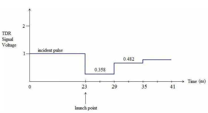
All previous calculated attributes will be the same in this scenario as previous, except for the effect of the water permittivity on probe impedance. For water, it will be assumed relative permittivity ε_r =K_a =81, therefore timing for the lower section transit can be made using (5.14) such that:

ns T

6 10 3

81 1 . 0 2

8

= ×

×

Also the impedance of the probe in soil can be found: Ω = = = 8 . 21 81 196 0 a probe pSoil K Z Z ... (5.22)

The reflection coefficient of the incident wave at the launch point can be determined by use of eqn. (5.1), such that:

642 . 0 2 2 0 0 1 − =             + − = Z Z Z Z pSoil pSoil ρ ... (5.23)

The transmission coefficient (using equ. 5.2) will be: 358 . 0 ) 1 ( 1

1= +ρ =

t ... (5.24)

The arrival of the first reflection back at the launch point experiences a different reflection shown in eqn. (5.3) asρ₂, and can be determined as:

179 . 0 0 0 0 0 2 − =               +       + −         + = pSoil Soil pSoil pSoil pSoil pSoil Z Zp Z Z Z Z Z Z Z Z ρ ... (5.25)

The second transmission coefficient (using eqn. 5.5) can now be determined as: 179

. 0

1 1 2

2 = +ρ +ρ =

t ... (