Robust rule-based prediction

Robust Rule-Based Prediction

Jiuyong Li

Abstract—This paper studies a problem of robust rule-based classification, i.e., making predictions in the presence of missing values in data. This study differs from other missing value handling research in that it does not handle missing values but builds a rule-based classification model to tolerate missing values. Based on a commonly used rule-based classification model, we characterize the robustness of a hierarchy of rule sets ask-optimalrule sets with the decreasing size corresponding to the decreasing robustness. We build classifiers based onk-optimalrule sets and show experimentally that they are more robust than some benchmark rule-based classifiers, such as C4.5rules and CBA. We also show that the proposed approach is better than two well-known missing value handling methods for missing values in test data.

Index Terms—Data mining, rule, classification, robustness.

æ

1

I

A

learning and data mining, and rule-based methods are widely accepted due to their easy understandability and interpretability. In the last 20 years, rule-based methods have been extensively studied, for example, C4.5rules [20], CN2 [7], [6], RIPPER [8], CBA [16], CMAR [15], and CPAR [23].

Most rule-based classification systems make accurate and understandable classifications. However, when a test data set contains missing values, a rule-based classification system may perform poorly because it may not be robust. We give the following example to show this.

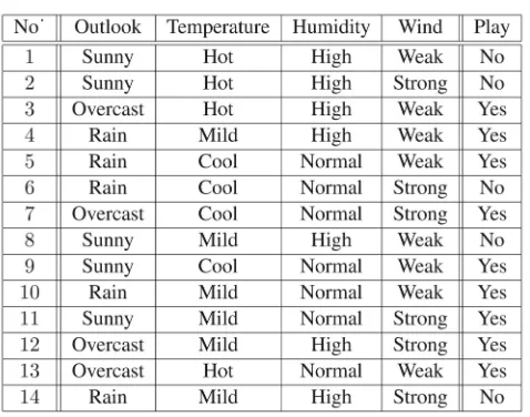
Example 1.Given a well-known data set listed in Table 1, a decision tree (e.g., ID3 [19] can be constructed as in Fig. 1.

The following five rules are from the decision tree:

1. If the outlook is sunny and humidity is high, then do not play tennis.

2. If the outlook is sunny and humidity is normal, then play tennis.

3. If the outlook is overcast, then play tennis. 4. If the outlook is rain and wind is strong, then do

not play tennis.

5. If the outlook is rain and wind is weak, then play tennis.

We note that all rules include the attribute outlook. Suppose that the outlook information is unknown in a test data set. This rule set makes no predictions on the test data set and, hence, is not robust. It is possible to have another rule set that makes some predictions on the incomplete test data set.

In real-world applications, missing values in data is very common. In many cases, missing values are unrecoverable due to unrepeatable procedures or the high cost of

experiments or surveys. Therefore, a practical rule-based classification system has to be robust for missing values.

One common way to deal with missing values is to estimate and replace them [18], called imputation. Some typical imputation methods are: mean imputation, predic-tion imputapredic-tion, and hot deck imputapredic-tion [3]. Imputapredic-tion methods are dominating in classification. For categorical attributes, the following three imputation methods are commonly used: most common attribute value substitution [7], local most common attribute value substitution [17], and multiple attribute value substitution [20]. In a recent study [3], the k-nearest neighbor substitution method is shown as the most accurate imputation method.

In this paper, we discuss an alternative approach for dealing with missing values. Instead of imputing missing values, we propose to build robust rule-based classification models to tolerate missing values. An imputation method is to “treat” missing values, but the proposed method is to make a system “immunize” from missing values to a certain degree.

Treating missing values can be effective when users know the data very well, but may lead to misleading predictions when a wrong value is imputed. For example, when a missing value female is imputed by value male, misleading prediction on the record may occur. In the worst case, the errors of a classification model and the errors of an imputation method are additive. In contrast, the proposed method does not impute missing values and, hence, does not incur errors from the missing value estimation.

We will discuss how to build robust rule-based classifiers that tolerate missing values. A rule-based classifier built on our method will be shown to be more accurate than two benchmark rule-based classifications systems, C4.5rules [20] and CBA [16] on incomplete test data sets. We also show that the classifier is more accurate than C4.5rules plus two imputation methods, respectively. A preliminary study appeared in [14], and this is a comprehensive report with a significant extension.

This paper primarily characterizes the relationships between the size of rule sets and their tolerative capability for missing values in test data. The theoretical conclusions . The author is with the Department of Mathematics and Computing, The

University of Southern Queensland, Toowoomba, 4350, Australia. E-mail: [email protected].

Manuscript received 4 Aug. 2005; revised 25 Jan. 2006; accepted 14 Mar. 2006; published online 19 June 2006.

For information on obtaining reprints of this article, please send e-mail to: [email protected], and reference IEEECS Log Number TKDE.

are very useful for selecting right rule sets to build rule-based classifiers. The paper also shows that building robust classifiers is a good alternative to handling missing values. The rest of the paper is organized as follows: Section 2 defines class association rules and their accuracies. Section 3 defines the optimal rule set and discusses its robustness. Section 4 defines k-optimal rule sets and discusses their robustness. Section 5 presents two algorithms to generate

k-optimal rule sets. Section 6 demonstrates that k-optimal

rule set-based classifiers are more robust than some bench-mark rule-based classifiers. Section 7 concludes the paper.

2

C

A

R

A

E

In this section, we define class association rules and discuss methods to estimate their accuracy.

Note that rules used for the final classifier are only a very small portion of a class association rule set. It is strongly argued that the optimal class association rule set [13] should be a proper base to build rule-based classifiers. In this paper, we start with the complete class association rule set and then move to the optimal class association rule set to

make the connection and distinction between our work and other works clear.

We use association rule concepts [1] to define class association rules. Given a relational data set D with

nattributes, a record of Dis a set of attribute-value pairs, denoted by T. An attribute is dedicated to class labels or every tuple has one class. A pattern is a set of attribute-value pairs. The support of a pattern P is the ratio of the number of records containingP to the number of records in the data set, denoted by suppðPÞ. An implication is a formula P!c, where P is a pattern and c is a class. The support of the implication P!c is suppðP[cÞ. The confidence of the implication is suppðP[cÞ=suppðPÞ, denoted by confðP!cÞ. The covered set of the rule is the set of all records containing the antecedent of the rule, denoted by covðP !cÞ. We say A!c is a class association rule if suppðA!cÞ and confðA!cÞ , where and are the minimum support and confidence, respectively.

Definition 1.The complete class association rule set is the set of all class association rules that satisfies the minimum support and the minimum confidence.

Given a data set D, the minimum support and the minimum confidence, the complete class association rule set is denoted byRcð; Þ, or simplyRc.

We list some frequently used notations of this paper in Table 2 for the fast referral.

TABLE 1 A Training Data Set

Fig. 1. A decision tree from the training data set.

TABLE 2

In classification study, the basic requirements of a rule are accuracy and coverage. More specifically, a rule covers few negative records in the training data set and identifies a certain number of records that have not been identified by other rules. The formal definition of “identify” will appear in the next section. A classification rule generation algo-rithm usually uses implicit minimum accuracy and support requirements. For example, the accuracy of a classification rule is generally very high, and those small coverage rules are more likely to be removed in the postpruning. Hence, the minimum thresholds in the above definition should not cause problems in practice.

In practice, predictions are made by a classifier. A classifier is a sequence of rules sorted by decreasing accuracy and tailed by a default prediction. In classifying an unseen record without class information, the first rule that matches the case classifies it. If no rule matches the record, the default prediction classifies it.

An estimation of rule accuracy is important since it directly affects how rules are used in the prediction. There are a few ways to estimate rule accuracy. Laplace accuracy is a widely used estimation [6]. We rewrite the Laplace accuracy in terms of support and cover set as follows:

LaplaceðA!cÞ ¼suppðA!cÞ jDj þ1 jcovðA!cÞj þ jCj ;

wherejCjis the number of all classes,suppðA!cÞ jDjis the number of correct predictions made by the rule on the training data and jcovðA!cÞj is the number of reords containing the antecedent of the rule in the training data.

Quinlan used the pessimistic error rate in rule pruning [20]. We present the pessimistic error as the pessimistic accuracy in the following:

PessimisticðA!cÞ ¼1fþ

z2

2Nþz

ffiffiffiffiffiffiffiffiffiffiffiffiffiffiffiffiffiffiffiffiffiffiffiffiffi f

N

f2

Nþ

z2

4N2

q

1þz2

N

;

where f¼1confðA!cÞ,N ¼ jcovðA!cÞj, andz is the standard deviation corresponding to a statistical confidence

c, which forc¼25%isz¼0:69.

Other interestingness metrics [21], such as the Chi-square test, can be used to compare predictive power of association rules. Our intention is not to discuss which estimation is the best in this paper. The accuracy of a rule can be estimated by a means. We represent the accuracy of rule A!c as

accðA!cÞ. We used Laplace accuracy in our experiments. Usually, the minimum confidence of a class association rule is high so it naturally excludes conflicting rules, such as

A!yandA!z, in a complete class association rule set. We will consistently discuss class association rules in the rest of the paper. For the sake of brevity, we omit class association in the following discussions.

3

T

O

R

S

I

R

3.1 Ordered Rule-Based Prediction Model and the Optimal Rule Set

In this section, we first formalize the procedure of rule-based classification and then define the optimal classifica-tion rule set.

We start with some notations. For a rule r, we use

condðrÞto represent its antecedent (conditions), andconsðrÞ

to denote its consequence. Given a test record T, we say rule r covers T ifcondðrÞ T. The set of records that are covered by a rule r is called the cover set of the rule, denoted by covðrÞ. A rule can make a prediction on a covered record. If consðrÞ is the class of T, then the rule makes a correct prediction. Otherwise, it makes a wrong prediction. Let the accuracy of a prediction equal the estimated accuracy of the rule making the prediction. If a rule makes the correct prediction on a record, then we say the ruleidentifiesthe record.

There are two types of rule-based classification models:

1. Ordered rule-based classifiers: Rules are organized as a sequence, e.g., in the descending accuracy order. When classifying a test record, the first rule covering the record in the sequence makes the prediction. This sequence is usually tailed by a default class (prediction). When there are no rules in the sequence covering the test record, the record is predicted to belong to the default class. C4.5rules [20] and CBA [16] employ this model.

2. Unordered rule-based classifiers: Rules are not organized in a sequence and all (or some) rules covering a test record participate in the determina-tion of the class of the record. A straightforward way is to adopt the majority vote of rules like in CPAR [23]. A more complex way is to build a model to compute the combined accuracy of multiple rules. Improved CN2 [6] and CMAR [15] employ this method.

We do not consider committee prediction, e.g., Bagging [5], which uses multiple classifiers.

The first model is simple and effective. It makes a prediction based on the maximum likelihood. This is because rules with higher accuracy usually precede rules with lower accuracy and the accuracy approximates the conditional probability when the data set is large.

There is no uniform form for the second model. Methods of voting vary in different proposals. An important condition for using the second model, independence of rules, is normally not satisfied. For example, in a complete class association rule set, the conditions of most rules are correlated. Further, voting may be bias against small distributed classes.

In this paper, we employ the ordered rule-based classification model. We formalize rule order as follows: Definition 2.Ruler1 precedes ruler2if:

1. accðr1Þ>accðr2Þ,

2. accðr1Þ ¼accðr2Þandsuppðr1Þ>suppðr2Þ, or

3. accðr1Þ ¼accðr2Þ,suppðr1Þ ¼suppðr2Þ, and

jcondðr1Þj<jconfðr2Þj:

this simple model to draw some theoretical conclusions, and then verify the conclusions by experiments.

A predictive rule is defined as follows:

Definition 3.LetTbe a record andRbe a rule set. RulerinRis the predictive rule forT ifrcoversT and is the most preceding rule among all rules coveringT.

For example, both rule ab!zðacc¼0:9Þ and rule d!

yðacc¼0:6Þ cover record fabcdeg. Rule ab!z is the predictive rule for the record but ruled!yis not.

As both the accuracy and the support are real numbers, in a large data set it is very unlikely that a record is covered by two rules with the same accuracy, support, and length. Therefore, it is a reasonable assumption that each record has a unique predictive rule for a given data set and a rule set, and we use this assumption in the rest of paper.

In the ordered rule-based classification model, only one rule makes prediction on a record and, hence, we have the following definition:

Definition 4.Let the prediction of rule set R on record T be the same as the prediction of the predictive rule inRon T.

For example, rule ab!zðacc¼0:9Þ predicts record

fabcdefgto belong to classzwith the accuracy of 90 percent. Rule set fab!zðacc¼0:9Þ; d!yðacc¼0:6Þg predicts re-cord fabcdefg to belong to class z with the accuracy of 90 percent since ruleab!zðacc¼0:9Þis the predictive rule. Some rules in the complete rule set never make predictions on any records, and we exclude them in the following.

First, we discuss how to compare predictive power of rules. We use r2r1 to represent condðr2Þ condðr1Þ and

consðr2Þ ¼consðr1Þ. We say thatr2ismore generalthanr1, or r1ismore specificthanr2. A rule covers a subset of records

covered by one of its more general rules.

Definition 5. Rule r2 is stronger than rule r1 if r2r1 and

accðr2Þ accðr1Þ. In a complete rule set Rc, a rule is

(maximally) strong if there is not another rule in Rc that is

stronger than it. Otherwise, the rule is weak.

Only strong rules make predictions in the complete rule set. For example, rule ab!z is weak because

accðab!zÞ<accða!zÞ. Whenever rule ab!z covers a record, rule a!z does. Since rule a!z precedes rule

ab!z, rule ab!z never has a chance to be a predictive rule. Therefore, we have the following definition to exclude weak rules like ab!z.

Definition 6.The set of all strong rules in the complete rule set is the optimal rule set, denoted byRopt.

A related concept of optimal rule set is nonredundant rule set. A definition of nonredundant association rule sets is presented by Zaki [24] and a nonredundant classification rule set is called an essential classification rule set [2]. The definition of essential classification rule sets is more restrictive than the definition of optimal rule sets. A more specific rule is excluded from an essential rule set only when both its support and its confidence are identical to those of one of its more general rules. The definition of the

optimal rule definition follows the observation that a more specific rule with accuracy lower than that of one of its more general rule does not participate in building an ordered rule-based classifier. An optimal rule set is a subset of the essential rule set. More detailed discussions on the relationships between optimal rule sets and nonredundant rule sets is characterized in my other work [12].

3.2 Robustness of the Optimal Rule Set

In this section, we first define robustness of rule sets and then discuss the robustness of the optimal rule set.

We use a concept of robustness to characterize the capability of rule set making predictions on incomplete data sets. We say that a rule set gives any prediction on a record with the accuracy of zero when it cannot provide a prediction on the record.

Definition 7.LetDbe a data set, andR1andR2be two rule sets

forD. R2 is at least as robust as R1 if, for all T0T and T 2D, predictions made byR2are at least as accurate as those

byR1.

For example, letR1¼ fab!zðacc¼0:9Þgand R2¼ fab!zðacc¼0:9Þ; d!zðacc¼0:8Þg:

For record fabcdeg, both rule sets predict it to belong to class z with the same accuracy of 90 percent. When b is missed from the record,R2 predicts it to belong to classz

with the accuracy of 80 percent whereas R1 predicts it to

belong to classzwith the accuracy of 0 percent. Thus,R2is

more robust thanR1.

For a large data set, estimated accuracies of rules approach true accuracies of rules. Consider that rule set

R2is more robust than rule setR1. For a complete test data

set both rule sets make predictions with the same accuracy. For an incomplete test data set, rule set R2 makes

predictions at least as accurately as rule setR1.

Ideally, we would like to have a rule set to make predictions on any incomplete record, but it is impossible since there may not be a rule in Rc covering every

incomplete record. The robustness of a rule set is limited by rules in Rc. On the other hand, this rule set is

unnecessarily large. The optimal rule set is a smaller equivalence.

Theorem 1.For any complete class association rule set Rc, the

optimal classification rule set Ropt is the smallest rule set in

size that is as robust asRc.

Proof. All weak rules excluded by the optimal rule set cannot be predictive rules in any cases because they are ordered lower and more specific than their correspond-ing strong rules that exclude them. On the other hand, every strong rule is a potentially predictive rule. When an incomplete record contains only the antecedent of a strong rule, the strong rule is the predictive rule for the record. Therefore, both the complete rule set and the optimal rule set have the same set of predictive rules and, hence, the optimal rule set is as robust as the complete rule set.

the new rule set R0o¼Roptnr is still as robust as the

complete rule set Rc. Consider a test record that is

covered only by rule r. By the definition of the optimal rule set, there is no rule inR0_o covering the record or at most there are some covering rules with a lower accuracy than r. Hence, the prediction made by R0

o cannot be as

accurate as that fromRopt. As a result,R0ois not as robust

asRc, and this contradicts the assumption.

The theorem is proved. tu

This theorem means that no matter what an input record is (complete or incomplete) the optimal rule set gives the same prediction on the record as the complete rule set with the same accuracy.

Let us look at differences between the complete rule set and the optimal rule set through an example.

Example 2.For the data set in Example 1, there are 21 rules in the complete rule set when the minimum support is

2=14 and the minimum confidence is 80 percent. However, there are only 10 rules in the optimal rule set, and they are listed as follows. We take confidence as accuracy in this example for easy illustration since, otherwise, an accuracy estimation method requires a calculator. (Numbers in parentheses are support and accuracy, respectively.)

1. If the outlook is sunny and humidity is high, then do not play tennis.ð3=14;100%Þ.

2. If the outlook is sunny and humidity is normal, then play tennis.ð2=14;100%Þ.

3. If the outlook is overcast, then play tennis.

ð4=14;100%Þ.

4. If the outlook is rain and wind is strong, then do not play tennis.ð2=14;100%Þ.

5. If the outlook is rain and wind is weak, then play tennis.ð3=14;100%Þ.

6. If humidity is normal and wind is weak, then play tennis. (3=14;100%).

7. If the temperature is cool and wind is weak, then play tennis. (2=14;100%).

8. If the temperature is mild and humidity is normal, then play tennis. (2=14;100%).

9. If the outlook is sunny and temperature is hot, then do not play tennis. (2=14;100%).

10. If humidity is normal, then play tennis. (6=14;87%).

Since the complete rule set is larger, we do not show it here. However, to demonstrate why some rules in the complete rule set are not predictive rules, we list seven rules including attribute value overcast as follows:

3. If the outlook is overcast, then play tennis.

ð4=14;100%Þ.

11. If the outlook is overcast and temperature is hot, then play tennis.ð2=14;100%Þ.

12. If the outlook is overcast and humidity is high, then play tennis.ð2=14;100%Þ.

13. If the outlook is overcast and humidity is normal, then play tennis.ð2=14;100%Þ.

14. If the outlook is overcast and wind is strong, then play tennis.ð2=14;100%Þ.

15. If the outlook is overcast and wind is weak, then play tennis.ð2=14;100%Þ.

16. If outlook is overcast and temperature is hot and wind is weak, then play tennis.ð2=14;100%Þ. Only rule 3 is included in the optimal rule set out of the above seven rules. The other six rules are not predictive rules since they follow rule 3 in the rule sequence defined by Definition 2 and are more specific than rule 3. Therefore, they cannot be predictive rules.

In the above example, the size difference between the complete rule set and the optimal rule set is not very significant because the underlying data set is very small. In some data sets, however, the optimal rule set can be less than 1 percent of the complete rule set.

Even though the optimal rule set is significantly smaller than the complete rule set, it is still much larger than a traditional classification rule set. Some rules in the optimal rule set are unnecessary when the number of missing attribute values is limited. Therefore, we show how to reduce the optimal rule set for a limited number of missing values in the following section.

4

k

-O

R

S

T

R

k-optimal rule sets for test data sets with up to k missing attribute values. We then discuss properties of k-optimal

rule sets.

We first define thek-incompletedata set to be a new data set with exactlyk missing values from every record of the data set. We usek-incompletedata sets as test data sets. Definition 8.LetDbe a data set withnattributes, andk0.

Thek-incompletedata set ofDis

Dk¼ fT0jT0T ; T2D;jTj jT0j ¼kg:

Conveniently,Dkconsists of a set of n_k data sets where each

omits exactlykattributes (columns) from D.

For example, the 1-incomplete data set contains a set of

ndata sets where each omits one attribute (column) fromD. Note that the 0-incomplete data set ofDisDitself.

Let us represent the optimal rule set in terms of incomplete data sets.

Lemma 1.The optimal rule set is the set of predictive rules for records in the union ofk-incompletedata sets for0k < n. Proof.First, a weak rule, excluded by the optimal rule set, cannot be a predictive rule for thek-incompleterecord. When a weak rule and one of its corresponding strong rules cover thek-incompleterecord, the strong rule will be the predictive rule. The weak rule is more specific than the strong rule and hence there is no chance for the weak rule to cover a record that is not covered by the strong rule.

record because other more general rules covering the record have lower accuracy than the strong rule.

Consequently, the lemma is proved. tu

In other words, if the optimal rule set could not make a prediction on an incomplete record, another rule set, e.g., the complete rule set, could not either; a rule in an optimal rule set is a predictive rule for some incomplete records. For example, given an optimal rule set

fa!zðacc¼0:9Þ; b!zðacc¼0:8Þ; c!zðacc¼0:7Þg:

For recordfabcdefgg, rulec!zbecomes the predictive rule when botha andbare missing.

The optimal rule set preserves all potential predictive rules fork-incompletedata sets withkup ton1. However, it is too big in many applications. Now, we consider how to preserve a small number of predictive rules for limited number of missing values in incomplete data sets.

Definition 9. A k-optimal rule set contains the set of all predictive rules on thek-incompletedata set.

For example, rule set fa!zðacc¼0:9Þ; b!zðacc¼

0:8Þgis 1-optimal for recordfabcdefgg. When ais missing, rule b!zis the predictive rule. When b,c,d,e,f, or gis missing, rulea!zis the predictive rule.

We have used the name of k-optimalrule sets in one of our previous work [14]. Recently, another rule mining algorithm [22] also generates k-optimal rule sets, which containkrules with the largest leverage.kin ourk-optimal

rule sets stands for k-missing values per record, and is usually a small number. kin the other k-optimal rule sets indicates the number of rules, and is a reasonably big number.

We have the following property fork-optimal rule sets. Lemma 2.Thek-optimalrule set makes the same predictions as

the optimal rule set on all p-incomplete data sets for

0pk.

Proof.Thek-optimalrule set contains predictive rules for all

p-incomplete data sets with 0pk according to Definition 9, and hence this lemma holds immediately.tu

For example, given an optimal rule set

fa!zðacc¼0:9Þ; b!zðacc¼0:8Þ; c!zðacc¼0:7Þ; d!zðacc¼0:6Þg:

Rule set fa!zðacc¼0:9Þ; b!zðacc¼0:8Þ; c!zðacc¼

0:7Þg is 2-optimal for recordfabcdefgg. It makes the same prediction as the optimal rule set on recordfabcdefggwith up to two missing values, e.g.fbcdefggandfcdefgg.

Thek-optimalrule set is a subset of the optimal rule set that makes the same predictions as the optimal rule set on a test data set withkmissing attribute values per record. As a special case, a 0-optimal rule set1 makes the same predictions as the optimal rule set on the complete test data set.

Theorem 2.Theðkþ1Þ-optimalrule set is at least as robust as thek-optimalrule set.

Proof.For those records inp-incompletedata sets forpk, both rule sets make the same predictions because both make the same predictions as the optimal rule set according to Lemma 2.

For those records in the ðkþ1Þ-incomplete data set, theðkþ1Þ-optimal rule set makes the same predictions as the optimal rule set and the k-optimal rule set does not. Hence, there may be some records that are identified by the ðkþ1Þ-optimal rule set but not by the k-optimal

rule set.

Consequently, theðkþ1Þ-optimalrule set is at least as robust as thek-optimal rule set. tu

For example, 2-optimal rule set fa!zðacc¼0:9Þ; b!

zðacc¼0:8Þ; c!zðacc¼0:7Þgis more robust than 1-opti-mal rule set fa!zðacc¼0:9Þ; b!zðacc¼0:8Þg. When valuesaandbare missed from the recordfabcdefgg, the first rule set predicts it to belong to classzwith the accuracy of 70 percent whereas the second rule set makes any prediction with the accuracy of 0 percent.

We give an example to showk-optimalrule sets and their predictive capabilities.

Example 3.In the data set of Example 1, with the minimum support of 2=14 and the minimum confidence of 80 percent, we have the optimal rule set with 10 rules as shown in Example 2. These 10 rules can identify all records in the data set. We take confidence as accuracy in this example for easy illustration since otherwise an accuracy estimation method requires a calculator. We have a min-optimal rule set as follows, where two numbers in the parentheses are support and accuracy, respectively:

1. If the outlook is sunny and humidity is high, then do not play tennis.ð3=14;100%Þ:

2. If the outlook is sunny and humidity is normal, then play tennis.ð2=14;100%Þ.

3. If the outlook is overcast, then play tennis.

ð4=14;100%Þ.

4. If the outlook is rain and wind is strong, then do not play tennis.ð2=14;100%Þ.

5. If the outlook is rain and wind is weak, then play tennis.ð3=14;100%Þ.

6. If humidity is normal and wind is weak, then play tennis. (3=14;100%).

Rules 1, 2, 3, 4, and 5 identify different records in the data set, so they are included in the min-optimal rule set. As to rule 6, it is the predictive rule for record 9. When identifying record 9, rule 6 has higher support than rule 2 and, hence, is the predictive rule for the record. This consideration results in that the min-optimal rule set is more robust than the rule set from the decision tree. When Outlook information is missing, the rule set from the decision tree identifies nothing while the min-optimal rule set identifies three records. The min-min-optimal rule set provides exactly the same predictions as the optimal rule set on the complete test data set.

With the following four additional rules, the rule set becomes 1-optimal.

7. If the temperature is cool and wind is weak, then play tennis. (2=14;100%).

8. If the temperature is mild and humidity is normal, then play tennis. (2=14;100%).

9. If the outlook is sunny and the temperature is hot, then do not play tennis. (2=14;100%).

10. If humidity is normal, then play tennis (6=14;87%).

This rule set gives more correct predictions on incomplete test data than the min-optimal rule set. For example, when Outlook information is missing, the 1-complete rule set identifies six records, which are three records more than the min-optimal rule set; when Temperature,14, equal; when Humidity,11,2more; and when Wind,11,2more. The improvement is clear and positive. In this example, the 1-optimal rule set equals the optimal rule set. This is because that the data set contains only four attributes. In most data sets, a 1-optimal rule set is significantly smaller than an optimal rule set.

Thek-optimalrule sets form a hierarchy.

Lemma 3. Let Rk and Rkþ1 be the k-optimal and the ðkþ

1Þ-optimalrule sets forD. Then,RkRkþ1.

Proof. Rk contains the set of all predictive rules over all p-incompletedata sets forpk.Rkþ1contains the set of

all predictive rules over allp-incompletedata sets forp

kand all predictive rules forðkþ1Þ-incompletedata sets. The predictive rule for a record is unique as assumed following Definition 3. So,RkRkþ1. tu

In Examples 2 and 3,Ropt¼R4¼R3¼R2¼R1Rmin.

Theoretically, k is up to n, the number of attributes, but practically, only a smallk << nis meaningful.

Until now, we have introduced the set of optimal rule sets, and we observe that the following hierarchy holds these optimal rule sets:

Ropt Rkþ1 Rk Rmin:

The robustness of ak-optimalrule set fork >0is due to that it preserves more potentially predictive rules in case that some rules are paralyzed by missing values in a data set. Usually, a traditional classification rule set is smaller than a min-optimal rule set, since most traditional classifi-cation systems postprune the final rule set to a small size. From our observations, most traditional classification rule sets are subsets of min-optimal rule sets. For example, the rule set from ID3 in Example 1 is a subset of the min-optimal rule set in Example 3 and is less robust than the min-optimal rule set. Experimental results will show this.

Finally, we consider a property that will help us to find

k-optimalrule sets. We can interpret thek-optimal rule set through a set of min-optimal rule sets.

Lemma 4. Consider that a k-incomplete sub data set omits exactlykattributes from data setD. The union of min-optimal rule sets over allk-incompletesub data sets isk-optimal.

Proof.For each of everyk-incompletesub data set, we obtain a min-optimal rule set that contains all predictive rules for the incomplete data set. The union of these min-optimal rule sets contains all predictive rules on the

k-incompletedata set, and hence isk-optimal. tu

We give an example to show this lemma.

Example 4.Follow Example 3. When Outlook information is omitted, a min-optimal rule set consists of rules 6, 7, 8, and 10; when Temperature, rules 1, 2, 3, 4, 5, and 6; when Humidity, rules 3, 4, 5, 7, and 9; when Wind, rules 1, 2, 3, 8, 9, and 10. The union of the above four min-optimal rule sets on four 1-incomplete data subsets is 1-optimal.

This lemma suggests that we can generate thek-optimal

rule set by generating min-optimal rule sets on a set of incomplete data sets.

5

C

k

-O

R

S

We now consider two different methods constructing robust rule sets. The first method extends a traditional classification rule generation technique and the second one extends an optimal classification rule mining technique.

5.1 A Multiple Decision Tree Approach

Heuristic methods have been playing an important role in classification problems, so here we first discuss how to generatek-optimalrule sets by a heuristic method.

In order to use a rule set on incomplete data sets, we may generate a rule set from an incomplete data set. For a set of

k-incompletesub data sets of the training data set, we can construct a set of rule sets on them. Intuitively, the union rule set will withstand up to k missing values to some extent.

We use C4.5rules [20] as the base rule generator in this algorithm. Although constructing multiple classifiers has been discussed before, such as Bagging [5] and Boosting [9], [10]. This algorithm differs from others in that it samples attributes systematically rather than records randomly, and that it uses the union of all rule sets instead of individual classifiers.

Thek-incompletedata set consists of a set of n

k (nis the

number of attributes for D) sub data sets in which each omits exactlykattribute (column) information from D.

Algorithm 1Multiple tree algorithm Input: data setD, integerk1

Output: Rule setR

(1) setR¼ ;

(2) for eachk-incompletesub data setD0ofD

(3) build a decision treeT fromD0by C4.5 (4) call C4.5rules to generate a rule setR0fromT

(5) letR¼R[R0

(6) returnR

We now study the robustness of the output rule set of the algorithm. Suppose that eachR0_{is the min-optimal rule set}

classification rule set is usually less robust than a min-optimal as shown in the experiments. Therefore, the output rule set is at most as robust as the k-optimalrule set.

This algorithm may be inefficient whenkis large. This is because n

k rule sets have to be generated where significant

repeating computation is involved. It is possible to modify codes of the C4.5 and C4.5rules to avoid the repeating computation. However, this modification may not be necessary when precisek-optimalrule sets can be generated.

5.2 An Optimal Class Association Rule Set Approach

In this section, we present a precise method to compute

k-optimal rule sets. A naive method would perform the following three steps:

1. Generate the complete rule set by an association rule approach, such as Apriori [1] or FP-growth [11]. 2. Find the min-optimal rule set for everyk-incomplete

data set.

3. Union all min-optimal rule sets.

This method would be inefficient. First, the complete rule set is usually very large, and is too expensive to compute for some data sets when the minimum support is low. Second, the process of finding the min-optimal rule set from a large complete rule set is expensive too.

An efficient algorithm [22] generatingk-optimalrule sets actually serves different purposes since that k-optimal is different from this k-optimal as discussions following Definition 9.

In our proposed algorithm, we directly find a smaller optimal rule set and compute thek-optimalrule set from the optimal class rule set in a single pass over the data set.

An efficient algorithm for generating the optimal rule set is presented in [13]. Here, we only present an algorithm to compute thek-optimalrule set from the optimal rule set.

Given a ruler, letAttrðrÞ be the set of attributes whose values appear in the antecedent ofr. Ap-attributepattern is an attribute set containing p attributes. Given a record T

and an attribute set X, let OmitðT ; XÞ be a new partial record projected fromT without attribute values fromX.

Algorithm 2k-optimalrule set generator

Input: data setD, optimal rule setRopt andk0

Output:k-optimalrule setR

(1) setR¼ ;

(2) for each recordTi inD

(3) letR0

i contain the set of rules that coverTi

(4) for eachr2R0

i letUsedAttr¼UsedAttr[AttrðrÞ

(5) for eachk-attributesetXinUsedAttr

(6) letT ¼OmitðTi; XÞ

(7) if there is no predictive rule forT inRi

(8) then select a predictive ruler0forT and move it fromR0_i intoRi

(9) letR¼RSRi

(10) returnR

We first illustrate the algorithm by the following example.

Example 5.Consider data set in Table 1 and the optimal rule set in Example 2. We use the above algorithm to generate the 1-optimal rule set. Let T1 be the first row

in Table 1. Initially, R¼ ; and R0

1¼ fr1; r9g, where r1

and r9 represent the first rule and the ninth rule in

the optimal rule set in Example 2. In line 4,

UsedAttr¼ fOutlook; T emperature; Humidityg. F r o m line 5 to line 8, first, the value in the Outlook column is omitted and no rule is selected. Second, the value in the Temperature column is omitted and the first rule r1 is selected. Third, the value in the Humidity

column is omitted and the ninth rule r9 is selected.

Up to line 9, R¼R1¼ fr1; r9g. Rule set fr1; r9g is the

1-optimal rule set for T1. As a comparison, rule set

fr1g is the min-optimal rule set for T1. For any one

missing value in T1, the min-optimal rule set has

50 percent of probability of being paralyzed by the missing value, either in the Outlook column or in the Humidity column, whereas the 1-optimal rule set has 25 percent of probability of being paralyzed by the missing value, only in the Outlook column. 1-optimal rule set reduces the probability of being paralyzed by missing values.

Now, we consider its correctness. In lines (4) and (5), we only consider attributes used in rules since missing values in other attributes do not affect the performance of rules. This algorithm selects predictive rules for all k-missing

patterns on each of every record in the training data set in lines (5) to (7). The algorithm generates ak-optimalrule set correctly according to Lemma 4.

6

E

In the previous sections, we built a theoretical model for selecting classification rule sets that were less sensitive to missing values in test data. In this section, we will experimentally prove that these rule sets do tolerate certain missing values in test data by showing their classification accuracies on incomplete test data. Missing values have not been handled, and we intend to show the ability of tolerating missing values of k-optimal rule sets and

k-optimalclassifiers.

In the first part of the experiments, we evaluate the robustness of k-optimal rule sets by following the defini-tions in the previous secdefini-tions except that a record in a

k-incomplete data set does not contain k missing values exactly, but on average.

In the second part of the experiments, we build classifiers based onk-optimalrule sets following a common practice in building rule-based classifiers. We compare our classifiers against two other benchmark rule-based classi-fiers on their classification performances on incomplete test data sets by using 10-fold cross validation. We also compare the proposed classifier with C4.5rules plus two well-known missing value handling methods.

6.1 Proof-of-Concept Experiment

In this section, we conduct an experiment to show the practical implication of definitions and theorems.k-optimal

data sets where 0l6. The l-incomplete data sets are different from Definition 8 since they contain l-missing

values on average rather than exactly.

Two data sets are selected from the UCI ML repository [4] and a brief description of them is in Table 4. They contain two classes each and their class distributions are relatively even. They are very easy to be classified by any classification method. We use them because they illustrate the main points of this paper very well.

k-optimalrule sets are generated by following algorithms 1 and 2. As a comparison, a traditional classification rule set is generated by C4.5rules [20].k-incompletetest data sets are generated by omitting on averagek values in each record. We control the total number of missing values, and let each record contain different number of missing values. To make the results reliable, we test every rule set on 10 randomly generated incomplete test data sets and report the average accuracy.

In the experiment, all rule sets are tested without the default predictions, since here we test robustness of rule sets rather than classifiers. Predictive rules are defined by Definition 3 using Laplace estimated accuracy. We set the minimum support as 0.1 in each class, called local support, minimum confidence as 0.5, and maximum rule length as 6 fork-optimal rule sets.

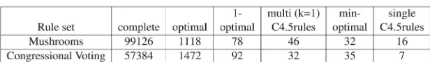
Table 3 shows that complete rule sets are significantly larger than optimal rule sets which are significantly larger than 1- and min-optimal rule sets. We observe the hierarchy of k optimal rule sets discussed in Section 4. Min-optimal rule sets are larger than rule sets from the C4.5rules [20]. Rule sets generated by multiple decision trees (k=1) are smaller than precise 1-optimal rule sets. This is because the C4.5rules prefers simple rule sets.

Fig. 2 shows that optimal rule sets perform the most accurately on incomplete test data, 1-optimal rule sets the second best, min-optimal rule sets the third, and rule sets from C4.5rules the worst. These results are consistent with Theorem 2. Rule sets from multiple C4.5rules (k=1) perform better than rule sets from single C4.5rules but worse than 1-optimal rule sets.

These results illustrate the main ideas in this paper very well. No rule set can be absolutely robust, but some rule sets are more robust than others. The robustness of

k-optimal rule sets follows Theorem 2. The reason for the robustness is that some additional rules are preserved in case other rules are paralyzed by missing values in the test data set.

We note that there is not big room for accuracy improvement between 1-optimal rule sets and optimal rule sets. Therefore, k-optimal rule sets for k >1 are

unnecessary. We also note that 1-optimal rule sets from the multiple decision tree approach are not as robust as precise 1-optimal rule sets. This is consistent with our analysis in Section 5.

6.2 Comparative Experiments

In this section, we conduct experiments to demonstrate the practical implication of the theoretical results in construct-ing robust rule-based classifiers. Different rule-based classifiers are tested on randomly generated incomplete test data sets where missing values have not been handled. The 10-fold cross validation method and 28 data sets have been employed in the experiments. A rule-based classifier that classifies incomplete test data with a higher accuracy is more robust than a rule-based classifier with a lower accuracy.

We construct k-optimal rule set-based classifiers by following a common practice for building rule-based classifiers. All rules in a k-optimal rule set are sorted by

TABLE 3

Sizes of Different Rule Sets

A complete rule set is very large, an optimal rule set is large, and a rule set from C4.5rules is very small. A 1-optimal rule set is larger than a min-optimal rule set. A rule set from multiple C4.5rules is closer to a min-min-optimal rule set than to a 1-min-optimal rule set.

their Laplace accuracy first. We then initiate an empty output rule sequence. We choose a rule with the minimum misclassification rate in thek-optimalrule set, and move this rule to the head of the output rule sequence. We remove the records covered by this rule, and compute the misclassifica-tion rate of remaining rules in thek-optimalrule set. Then, we recursively move the rule with the minimum misclassi-fication rate to the tail of output rule sequence until there is no record left. When there are two rules with the same misclassification rate, the preceding rule in the k-optimal

rule set is removed. After the above procedure is finished, remaining rules in the k-optimal rule set are appended to the output rule sequence in the order of Laplace accuracy. The majority class in the data set is set as the default class. All k-optimal classifiers are compared against two benchmark rule-based classifiers, C4.5rules [20] and CBA [16]. The former is a typical decision tree-based classifier, and the latter is an association-based classifier. We do not include the multiple decision tree approach since a 1-optimal rule set from the multiple decision tree approach is not as robust as a precise 1-optimal rule set as shown by our analysis and experiment. Further, the multiple decision tree approach is too time consuming whenk >1.

Twenty-eight data sets from UCI ML Repository [4] are used to evaluate the robustness of different classifiers. A

summary of these data sets is given in Table 4. The 10-fold cross validation method is used in the experiment.

k-incomplete test data sets are generated by randomly omitting values in test data sets so that each record has on averagek-missingvalues. Because thek-incompletetest data sets are generated randomly, the accuracy of each fold of 10-fold cross validation is the average of accuracies obtained from 10 tests.

The parameters for the optimal rule set generation are listed as follows: Local minimum support (support in a class), 0.01, minimum confidence, 0.5, and maximum length of rules, 6. For both C4.5rules and CBA, we used their default settings.

Fig. 3 shows that an optimal classifier is significantly larger than both CBA and C4.5rules classifiers. A CBA classifier approaches a min-optimal classifier in size. A C4.5rules classifier is the smallest. A 1-optimal classifier is nearly twice as large as a min-optimal classifier.

Fig. 4 shows that optimal, 1-optimal, and min-optimal classifiers are more accurate than both CBA and C4.5rules classifiers on incomplete test data sets. Therefore, all optimal classifiers are more robust than CBA and C4.5rules classifiers.

The accuracy differences in Fig. 4 is not so significant because the accuracies have been floated by the default predictions. A test record covered by no rule in a classifier is Fig. 2. The robustness of different rule sets. Optimal rule sets are the more robust, 1-optimal rule sets the second, min-optimal rule set the third, and rule sets from C4.5rules the least robust. Rule sets from multiple C4.5rules are more robust than rule sets from single C4.5rules, but less robust than 1-optimal rule sets.

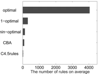
Fig. 3. The average sizes of different classifiers on 28 data sets. An optimal classifier is large whereas a C4.5rules classifier is very small. A CBA classifier is close to a min-optimal classifier, and both are smaller than a 1-optimal classifier.

predicted to belong to the default class. The default prediction makes a classifier simple but may disguise the true accuracy. For example, in data set Hypothyroid, 95.2 percent records belong to class Negative and only 4.8 percent records belong to class Hypothyroid. So, if we set the default prediction as Negative, then this classifier will give 95.2 percent accuracy on a test data set that misses all values. The true accuracy for this “empty” data set should be zero rather than 95.2 percent. We see that how the accuracy is floated by the default prediction. Further, this distribution knowledge is too general to be useful. For example, a doctor uses his patient data to build a rule-based diagnosis system. Eighty percent of patients coming to see him are healthy and, hence, the system sets the default as healthy. Though the default easily picks up 80 percent accuracy, this accuracy is meaningless for the doctor.

In the following experiments, we remove the default prediction from each classifier. We repeat the same experiment for all classifiers without the default predictions and report the average accuracies on Fig. 5. CBA has not been included because we could not remove its default prediction.

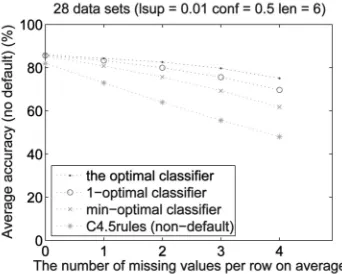
Fig. 6 shows that all optimal classifiers are more accurate than C4.5rules classifiers on incomplete data, and hence are more robust. Optimal classifiers are more robust than 1-optimal classifiers, which are more robust than min-optimal classifiers on average. Optimal classifiers improve classification accuracies on incomplete test data by up to 28.2 percent over C4.5rules classifiers without the default predictions. This is a significant improvement.

By comparing size differences of optimal, 1-optimal, and min-optimal classifiers with their classification accuracy differences on incomplete test data, 1-optimal classifiers make use of rules effectively.

To show the advantages of building robust classifiers over imputing missing values, we compare the robust rule-based classifiers to C4.5rules plus two different missing value imputing methods. Most common attribute value substitution is a simple but effective approach for imputing missing categorical values [7]. k-nearest neighbor substitu-tion is the most accurate approach for imputing missing values as shown in the recent work [3]. In the former

approach, a missing value is replaced by a value that occurs most frequently in an attribute. In the later approach, a missing value is replaced by a value that occurs most frequently in its k-nearest neighborhood.

We compare the proposed robust classifier, e.g., 1-optimal classifier without handling missing values, to C4.5rules with test values being imputed by both ap-proaches. In the k-nearest neighbor substitution,kis set as 10 as in [3]. When the size of a test data set is smaller than 100 but greater than 30,kis set as 5. When the size of a test data set is smaller than 30,kis set as 3.

Fig. 6 shows that 1-optimal classifier alone is more accurate than C4.5rules plus most common attribute substitution and k nearest neighbor substitution, respec-tively. This demonstrates that building robust rule-based classifiers is better than treating missing values. In addition, 1-optimal classifier also benefits from a good imputation method. When the average missing values in each record exceeds two in our experiments, k-nearest neighbor sub-stitution method improves the accuracy of 1-optimal classifier.

7

C

In this paper, we discussed a problem of selecting rules to build robust classifiers that tolerate certain missing values in test data. It differs from a missing value handling problem since our discussion is about “immunizing” from the missing values rather than “treating” missing values. We defined a hierarchy of optimal rule sets,k-optimalrule sets, and concluded that the robustness of k-optimal rule sets decreases with the decreasing size of rule sets. We proposed two methods to findk-optimal sets. We demon-strated the practical implication of the theoretical results by extensive experiments. All optimal rule set-based classifiers are more robust than two benchmark rule-based classifica-tion systems, C4.5rules and CBA. We further show that the proposed method is better than two well-known missing value handling methods for missing values in test data.

Given the frequent missing values in real-world data,

k-optimal rule sets have great potential in building robust Fig. 5. The average accuracies of four classifiers without the default

predictions on 28 data sets. Optimal rule classifiers are the most robust, 1-optimal classifiers the second, min-optimal classifiers the third, and C4.5rules classifiers the least robust.

classifiers in the future applications. The theoretical results also provide a guideline for pruning rules in a large rule set.

A

The author thanks Professor Rodney Topor and Professor Hong Shen for their constructive discussions and comments on the preliminary work. He also thanks the anonymous reviewers for their constructive suggestions, Hong Hu for conducting some comparative experiments, Ron House for proofreading this paper, Ross Quinlan for making C4.5 available for research, and Bing Liu for providing CBA for the comparison. This project was supported by ARC (Australia Research Council) grant DP0559090.

R

[1] R. Agrawal and R. Srikant, “Fast Algorithms For Mining Association Rules In Large Databases,”Proc. 20th Int’l Conf. Very Large Databases,pp. 487-499, 1994.

[2] E. Baralis and S. Chiusano, “Essential Classification Rule Sets,”

ACM Trans. Database Systems,vol. 29, no. 4, pp. 635-674, 2004.

[3] G.E.A.P.A. Batista and M.C. Monard, “An Analysis of Four Missing Data Treatment Methods for Supervised Learning,”

Applied Artificial Intelligence,vol. 17, nos. 5-6, pp. 519-533, 2003.

[4] E.K. C. Blake and C.J. Merz UCI Repository of Machine Learning Databases, http://www.ics.uci.edu/~mlearn/MLRepository. html, 1998.

[5] L. Breiman, “Bagging Predictors,” Machine Learning, vol. 24, pp. 123-140, 1996.

[6] P. Clark and R. Boswell, “Rule Induction with CN2: Some Recent Improvements,”Machine Learning-EWSL-91,pp. 151-163, 1991.

[7] P. Clark and T. Niblett, “The CN2 Induction Algorithm,”Machine Learning,vol. 3, no. 4, pp. 261-283, 1989.

[8] W.W. Cohen, “Fast Effective Rule Induction,”Proc. 12th Int’l Conf. Machine Learning (ICML),pp. 115-123, 1995.

[9] Y. Freund and R.E. Schapire, “Experiments with a New Boosting Algorithm,”Proc. Int’l Conf. Machine Learning,pp. 148-156, 1996.

[10] Y. Freund and R.E. Schapire, “A Decision-Theoretic General-ization of On-Line Learning and an Application to Boosting,”

J. Computer and System Sciences,vol. 55, no. 1, pp. 119-139, 1997.

[11] J. Han, J. Pei, and Y. Yin, “Mining Frequent Patterns without Candidate Generation,” Proc. 2000 ACM-SIGMOD Int’l Conf. Management of Data (SIGMOD ’00),pp. 1-12, May 2000.

[12] J. Li, “On Optimal Rule Discovery,” IEEE Trans. Knowledge and Data Eng.,vol. 18, no. 4, pp. 460-471, 2006.

[13] J. Li, H. Shen, and R. Topor, “Mining the Optimal Class Association Rule Set,” Knowledge-Based System, vol. 15, no. 7, pp. 399-405, 2002.

[14] J. Li, R. Topor, and H. Shen, “Construct Robust Rule Sets for Classification,” Proc. Eighth ACMKDD Int’l Conf. Knowledge Discovery and Data Mining,pp. 564-569, 2002.

[15] W. Li, J. Han, and J. Pei, “CMAR: Accurate and Efficient Classification Based on Multiple Class-Association Rules,” Proc. 2001 IEEE Int’l Conf. Data Mining (ICDM ’01),pp. 369-376, 2001.

[16] B. Liu, W. Hsu, and Y. Ma, “Integrating Classification and Association Rule Mining,” Proc. Fourth Int’l Conf. Knowledge Discovery and Data Mining (KDD ’98),pp. 27-31, 1998.

[17] J. Mingers, “An Empirical Comparison of Selection Measures for Decision Tree Induction,” Machine Learning,vol. 3, pp. 319-342, 1989.

[18] D. Pyle,Data Preparation for Data Mining.San Francisco: Morgan Kaufmann, 1999.

[19] J.R. Quinlan, “Induction of Decision Trees,” Machine Learning,

vol. 1, no. 1, pp. 81-106, 1986.

[20] J.R. Quinlan, C4.5: Programs for Machine Learning. San Mateo, Calif.: Morgan Kaufmann, 1993.

[21] P. Tan, V. Kumar, and J. Srivastava, “Selecting the Right Objective Measure for Association Analysis,” Information Systems,vol. 29, no. 4, pp. 293-313, 2004.

[22] G.I. Webb and S. Zhang, “K-Optimal Rule Discovery,” Data Mining and Knowledge Discovery J.,vol. 10, no. 1, pp. 39-79, 2005.

[23] X. Yin and J. Han, “CPAR: Classification Based on Predictive Association Rules,”Proc. 2003 SIAM Int’l Conf. Data Mining (SDM ’03),2003.

[24] M.J. Zaki, “Mining Non-Redundant Association Rules,” Data Mining and Knowledge Discovery J.,vol. 9, pp. 223-248, 2004.

Jiuyong Lireceived the BSc degree in physics and the MPhil degree in electronic engineering from Yunna University in China in 1987 and 1998, respectively, and received the PhD degree in computer science from Griffith Uni-versity in Australia in 2002. He is currently a lecturer at the University of Southern Queens-land in Australia. His main research interests are in data mining and bioinformatics.