Theses
2-15-2019
Efficient Nonlinear Dimensionality Reduction for
Pixel-wise Classification of Hyperspectral Imagery
Xuewen Zhang
Follow this and additional works at:
https://scholarworks.rit.edu/theses
This Dissertation is brought to you for free and open access by RIT Scholar Works. It has been accepted for inclusion in Theses by an authorized administrator of RIT Scholar Works. For more information, please [email protected].
Recommended Citation
by
Xuewen Zhang
B.S. Harbin Institute of Technology, 2010
M.S. Harbin Institute of Technology, 2012
A dissertation submitted in partial fulfillment of the
requirements for the degree of Doctor of Philosophy
in the Chester F. Carlson Center for Imaging Science
College of Science
Rochester Institute of Technology
February 15, 2019
Signature of the Author
Accepted by
ROCHESTER INSTITUTE OF TECHNOLOGY
ROCHESTER, NEW YORK
CERTIFICATE OF APPROVAL
Ph.D. DEGREE DISSERTATION
The Ph.D. Degree Dissertation of Xuewen Zhang has been examined and approved by the dissertation committee as satisfactory for the
dissertation required for the Ph.D. degree in Imaging Science
Dr. Nathan Cahill, Dissertation Advisor Date
Dr. David Messinger Date
Dr. John Kerekes Date
Dr. Kara Maki Date
COLLEGE OF SCIENCE
CHESTER F. CARLSON CENTER FOR IMAGING SCIENCE
Title of Dissertation:
Efficient Nonlinear Dimensionality Reduction
for Pixel-wise Classification of Hyperspectral Imagery
I, Xuewen Zhang, hereby grant permission to Wallace Memorial Library of R.I.T. to
reproduce my thesis in whole or in part. Any reproduction will not be for commercial
use or profit.
Signature
Date
by
Xuewen Zhang
Submitted to the
Chester F. Carlson Center for Imaging Science in partial fulfillment of the requirements
for the Doctor of Philosophy Degree at the Rochester Institute of Technology
Abstract
Classification, target detection, and compression are all important tasks in analyzing
hyper-spectral imagery (HSI). Because of the high dimensionality of HSI, it is often useful to identify
low-dimensional representations of HSI data that can be used to make analysis tasks tractable.
Traditional linear dimensionality reduction (DR) methods are not adequate due to the
nonlin-ear distribution of HSI data. Many nonlinnonlin-ear DR methods, which are successful in the general
data processing domain, such as Local Linear Embedding (LLE) [1], Isometric Feature
Map-ping (ISOMAP) [2] and Kernel Principal Components Analysis (KPCA) [3], run very slowly
and require large amounts of of memory when applied to HSI. For example, applying KPCA to
the 512×217 pixel, 204-band Salinas image using a modern desktop computer (AMD FX-6300
Six-Core Processor, 32 GB memory) requires more than 5 days of computing time and 28GB
memory!
In this thesis, we propose two different algorithms for significantly improving the
computa-tional efficiency of nonlinear DR without adversely affecting the performance of classification
task: Simple Linear Iterative Clustering (SLIC) superpixels and semi-supervised deep
autoen-coder networks (SSDAN). SLIC is a very popular algorithm developed for computing
superpix-els in RGB images that can easily be extended to HSI. Each superpixel includes hundreds or
thousands of pixels based on spatial and spectral similarities and is represented by the mean
spectrum and spatial position of all of its component pixels. Since the number of superpixels is
much smaller than the number of pixels in the image, they can be used as input for nonlinear
DR, which significantly reduces the required computation time and memory versus providing all
of the original pixels as input. After nonlinear DR is performed using superpixels as input, an
interpolation step can be used to obtain the embedding of each original image pixel in the low
dimensional space. To illustrate the power of using superpixels in an HSI classification pipeline,
we conduct experiments on three widely used and publicly available hyperspectral images:
In-dian Pines, Salinas and Pavia. The experimental results for all three images demonstrate that
for moderately sized superpixels, the overall accuracy of classification using superpixel-based
nonlinear DR matches and sometimes exceeds the overall accuracy of classification using
pixel-based nonlinear DR, with a computational speed that is two-three orders of magnitude faster.
Even though superpixel-based nonlinear DR shows promise for HSI classification, it does
have disadvantages. First, it is costly to perform out-of-sample extensions. Second, it does not
generalize to handle other types of data that might not have spatial information. Third, the
original input pixels cannot approximately be recovered, as is possible in many DR algorithms.
In order to overcome these difficulties, a new autoencoder network - SSDAN is proposed. It is a
fully-connected semi-supervised autoencoder network that performs nonlinear DR in a manner
that enables class information to be integrated. Features learned from SSDAN will be similar
to those computed via traditional nonlinear DR, and features from the same class will be close
to each other. Once the network is trained well with training data, test data can be easily
mapped to the low dimensional embedding. Any kind of data can be used to train a SSDAN,
and the decoder portion of the SSDAN can easily recover the initial input with reasonable loss.
Experimental results on pixel-based classification in the Indian Pines, Salinas and Pavia images
show that SSDANs can approximate the overall accuracy of nonlinear DR while significantly
features of a trained SSDAN for a new HSI dataset. Finally, experimental results on HSI
compression show a trade-off between Overall Accuracy (OA) of extracted features and Peak
Signal to Noise Ratio (PSNR) of the reconstructed image.
Keywords: hyperspectral image, nonlinear dimensionality reduction, autoencoder,
First of all, I want to thank RIT and the Chester F. Carlson Center for Imaging Science
for offering me admission to the Imaging Science Ph.D Program, and for providing teaching
assistantships and research assistantships. Without them, I would not have been able to carry
out my Ph.D in the US.
Next, I want to offer my sincerest gratitude to my advisor, Nathan D. Cahill. During my
five years as a Ph.D. student, you always supported me and my dreams. You gave me a lot of
advice for my life, my courses, and my research, and you also show me the culture of America.
Your passion in math, coding and research impresses me a lot. Whenever I have troubles in my
research, you are so patient and professional and give me strength to help me overcome those
troubles. I can’t forget that you have helped me revise many abstracts, proposals, and papers.
You are my good friend, advisor, and mentor in my whole life.
I would like to thank all of my colleagues in the research team: Tyler Hayes, Renee Meinhold,
Selene Chew and Eman Johnson. Thanks to all of you for offering me advice and smiles during
our conversations. And I’m also very overwhelmed with longing for those days of attending the
SPIE conference together with you.
I would also like to thank all of my colleagues in the office: Zhenlin Xu, Chi Zhang, Geifei
Yang and Kamal Jnawali. Thanks to all of you for accompanying me for so many days in the
office. When I have a question, you help me answer it. When I have good news, I want to share
it with you. You are very good people.
My gratitude also goes to all of my friends in Rochester: Zhaoyu Cui, Fan Wang, Runchen
Zhao, Wei Yao, Can Jin, Chao Zhang, Fei Zhang and Yawen Lu. Thanks for your advice on my
Ph.D and on the following career. I hope we can be still good friends in my following life.
Finally, I want to thank my family: my wife Runzi Wang, my daughter Emily Zhang, my
mother Haiyan Chen and my father Hengsheng Zhang, for your support and understanding.
I’m happiest when I see you live happily. Thanks for all the moments we shared together.
1 Introduction 18
2 Background 20
2.1 Hyperspectral imaging (HSI) . . . 20
2.2 HSI Analysis Tasks . . . 24
2.2.1 Pixel-based Classification . . . 24
2.2.2 Target Detection . . . 25
2.2.3 Compression . . . 27
2.3 Dimensionality Reduction for HSI . . . 28
2.3.1 Linear Dimensionality Reduction . . . 29
2.3.2 Nonlinear Dimensionality Reduction . . . 30
2.4 Example Nonlinear DR Methods . . . 36
2.4.1 Spatial Spectral Schroedinger Eigenmaps (SSSE) . . . 36
2.4.2 Kernel Principle Component Analysis (KPCA) . . . 39
2.5 Summary . . . 42
3 Superpixel-based Dimensionality Reduction of HSI 43 3.1 Review of Superpixel Construction Techniques . . . 44
3.2 Simple Linear Iterative Clustering (SLIC) . . . 45
3.3 Applications of Superpixels in HSI . . . 47
3.4 Proposed HSI Classification Framework . . . 52
3.5 Experiments . . . 53
3.5.1 Data sets . . . 53
3.5.2 Experimental setup . . . 54
3.5.3 Results . . . 56
3.6 Conclusion . . . 74
4 Semi-Supervised Deep Autoencoder Networks 75 4.1 Autoencoders . . . 76
4.1.1 Background . . . 77
4.1.2 Applications . . . 83
4.2 Proposed Autoencoder Network: SSDAN . . . 87
4.3 Pixel-wise HSI Classification Experiments . . . 90
4.3.1 Experimental Setup . . . 90
4.3.2 Comparison with Other Methods . . . 91
4.3.3 Data augmentation . . . 93
4.3.4 Effectiveness of the loss function . . . 95
4.3.5 Different activations . . . 98
4.3.6 Different numbers of layers . . . 98
4.3.7 Different numbers of neurons . . . 99
4.3.8 Different dimensions . . . 100
4.3.9 Different number of training samples . . . 101
4.3.10 Transfer learning . . . 102
4.4 HSI Compression Experiments . . . 106
4.5 Summary . . . 112
5.2.1 HSI classification . . . 116
5.2.2 HSI target/anomaly detection . . . 116
5.2.3 Regular image compression . . . 117
5.2.4 Modify the loss function for GAN . . . 117
5.2.5 Convolutional network to simulate nonlinear DR method . . . 118
Appendices 119
List of Figures
2.1 An illustration of an HSI scene, taken from [4]. In the figure, the sun, air, tank and satellite correspond to the four basic elements in the hyperspectral remote sensing system: source, atmospheric path, target and sensor. . . 222.2 Schematic diagram of HSI spectrometer, taken from [5]. Many detector arrays are used to measure reflectance with different locations and bands. . . 22
2.3 Schematic illustration of a hyperspectral image as a ”cube” of data. Tens or hundreds of narrow bands (different layers in the image . . . 23
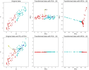
2.4 PCA and KPCA results for linear data. In the left column, the original data and PCs in PCA are shown. In the middle column, the results of PCA in 2-D and 1-D are shown. In the right column, the results of KPCA in 2-D and 1-D are shown. . . 32
2.5 PCA and KPCA results for nonlinear data1. In the left column, the original data
and PCs in PCA are shown. In the middle column, the results of PCA in 2-D
and 1-D are shown. In the right column, the results of KPCA in 2-D and 1-D
are shown. Figure from [6]. . . 33
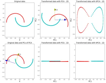
2.6 PCA and KPCA results for nonlinear data2. In the left column, the original data
and PCs in PCA are shown. In the middle column, the results of PCA in 2-D
and 1-D are shown. In the right column, the results of KPCA in 2-D and 1-D
are shown. Figure from [6]. . . 34
2.7 DR results for S-shaped Data. In the leftmost column, the 3-D original S-shaped
data is shown. Eight DR results are shown in the right including PCA and seven
nonlinear DR results. Figure from [7]. . . 35
3.1 Left: Indian Pines image (spectral bands 29, 15, 12) and manually labeled
refer-ence data (16 classes). Right: SLIC superpixels for various choices ofs(superpixel
size) andr (superpixel regularity). . . 48
3.2 Left: Salinas image (spectral bands 29, 15, 12) and manually labeled reference
data (16 classes). Right: SLIC superpixels for various choices of s (superpixel
size) andr (superpixel regularity). . . 49
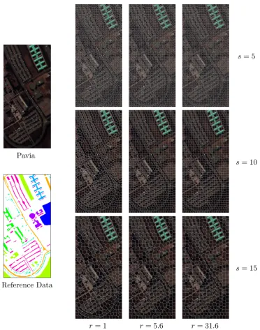
3.3 Left: Pavia image (spectral bands 48, 17, 6) and manually labeled reference data
(9 classes). Right: SLIC superpixels for various choices ofs(superpixel size) and
r (superpixel regularity). . . 50
3.4 Pipeline of proposed method for pixel-wise HSI classification. . . 53
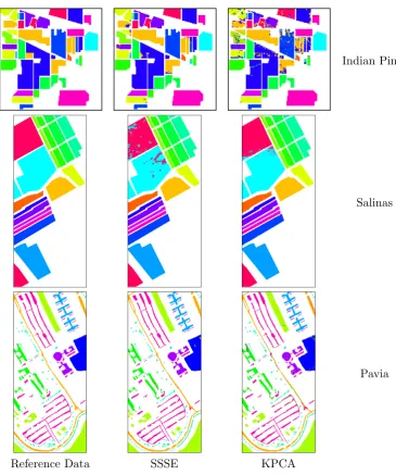
3.5 Reference data and class maps from classification of Indian Pines, Salinas, and
Pavia imagery using SSSE and KPCA embeddings computed from original image
3.6 Overall classification accuracy (top) and computation time (bottom) as
super-pixel size (s) varies for SLIC superpixel-based nonlinear DR via SSSE (left) and
KPCA (right) on Indian Pines. . . 59
3.7 Overall classification accuracy (top) and computation time (bottom) as
super-pixel size (s) varies for SLIC superpixel-based nonlinear DR via SSSE (left) and
KPCA (right) on Salinas. . . 61
3.8 Overall classification accuracy (top) and computation time (bottom) as
super-pixel size (s) varies for SLIC superpixel-based nonlinear DR via SSSE (left) and
KPCA (right) on Pavia. . . 62
3.9 Overall classification accuracy (top) and computation time (bottom) as
super-pixel regularity (r) varies for SLIC superpixel-based nonlinear DR via SSSE (left)
and KPCA (right) on Indian Pines. . . 63
3.10 Overall classification accuracy (top) and computation time (bottom) as
super-pixel regularity (r) varies for SLIC superpixel-based nonlinear DR via SSSE (left)
and KPCA (right) on Salinas. . . 64
3.11 Overall classification accuracy (top) and computation time (bottom) as
super-pixel regularity (r) varies for SLIC superpixel-based nonlinear DR via SSSE (left)
and KPCA (right) on Pavia. . . 65
3.12 Left: Indian Pines reference data; right: Classification maps based on SSSE
embeddings computed with SLIC superpixels for various choices of s (size) and
r (regularity). . . 66
3.13 Left: Indian Pines reference data; right: Classification maps based on KPCA
embeddings computed with SLIC superpixels for various choices of s (size) and
3.14 Left: Salinas reference data; right: Classification maps based on SSSE
embed-dings computed with SLIC superpixels for various choices of s(size) andr
(reg-ularity). . . 68
3.15 Left: Salinas reference data; right: Classification maps based on KPCA
em-beddings computed with SLIC superpixels for various choices of s (size) and r
(regularity). . . 69
3.16 Left: Pavia reference data; right: Classification maps based on SSSE embeddings
computed with SLIC superpixels for various choices of s(size) and r (regularity). 70
3.17 Left: Pavia reference data; right: Classification maps based on KPCA
embed-dings computed with SLIC superpixels for various choices of s(size) andr
(reg-ularity). . . 71
4.1 Structure of an autoencoder network with three hidden layers. Figure from [8]. . 78
4.2 SSDAN Structure . . . 88
4.3 Flowchart showing the use of a SSDAN as a preprocessing step for classification. 89
4.4 Left: reference data of Indian Pines; middle: Classification maps for
SSDAN-based SSSE method of Indian Pines; right: Classification maps for SSDAN-SSDAN-based
KPCA method of Indian Pines. . . 93
4.5 Left: reference data of Salinas; middle: Classification maps for SSDAN-based
SSSE method of Salinas; right: Classification maps for SSDAN-based KPCA
method of Salinas. . . 94
4.6 Left: reference data of Pavia; middle: Classification maps for SSDAN-based SSSE
method of Pavia; right: Classification maps for SSDAN-based KPCA method of
4.7 OA of pixel-based HSI classification when different numbers of sub-loss terms
are used. One sub-loss: autoencoder loss; two sub-losses: autoencoder + mean
loss; three sub-losses: autoencoder + mean + manifold loss; four sub-losses:
autoencoder + mean + manifold + class loss. . . 97
4.8 OA of pixel-based HSI classification when different coefficient values are chosen
for each sub-loss term. . . 98
4.9 OA of pixel-based HSI classification using SSDANs with different activation
func-tions. . . 99
4.10 OA of pixel-based HSI classification using SSDANs with different numbers of layers.100
4.11 OA of pixel-based HSI classification using SSDAN with different numbers of
neurons. . . 101
4.12 OA of pixel-based HSI classification using SSDAN with different feature dimensions.101
4.13 OA of pixel-based HSI classification using SSDANs as a function of different
training set sizes. . . 102
4.14 The Berlin pseudo-color image (spectral bands 2, 4, 6 in Landsat 8) and manually
labeled reference data (11 classes). . . 105
4.15 The Paris pseudo-color image (spectral bands 1, 3, 5 in Landsat 8) and manually
labeled reference data (12 classes). . . 105
4.16 OA of pixel-based HSI classification using SSDANs with transfer learning. . . 106
4.17 The original and recovered data . . . 107
4.18 PSNR and CR versus OA of pixel-based HSI classification for Indian Pines,
Sali-nas and Pavia. . . 109
4.19 Histogram of mean square error (MSE) for all of the pixels in Indian Pines,
PCA reconstruction error and right column corresponds to SSDAN reconstruction
error. . . 111
List of Tables
3.1 Names and the number of samples for each reference data class from each image. 54 3.2 Definitions of per-class classification performance measures, in terms of true pos-itives (TP), false pospos-itives (FP), false negatives (FN), and true negatives (TN). . 553.3 Baseline classification results for Indian Pines, Salinas, and Pavia, without using superpixels. Performance measures include precision (Pr), sensitvity (Se), overall accuracy (OA), average accuracy (AA), kappa coefficient (κ), and computing time. 58 3.4 Comparison with state-of-the-art classification methods on Indian Pines . . . 73
3.5 Comparison with state-of-the-art classification methods on Salinas . . . 73
3.6 Comparison with state-of-the-art classification methods on Pavia . . . 74
4.1 Results of pixel-wise classification using original HSI data, and using low-dimensional embeddings constructed from PCA, traditional SSSE, traditional KPCA, SSDAN-KPCA and SSDAN-SSSE. . . 93
4.2 Results of different data augmentation methods for SSDAN-SSSE. . . 96
4.3 Results of different data augmentation methods for SSDAN-KPCA. . . 96
4.4 Number of neurons in each layer of encoder network . . . 99
4.5 Number of neurons in each layer of encoder network . . . 100
4.6 Names and the number of samples for each reference class in Berlin and Paris
image. . . 113
4.7 Fraction of variance for PCA . . . 113
1 Confusion matrix of superpixel-based SSSE method with s = 15 and r = 1 for
Indian Pines. Rows correspond to the reference data and columns correspond to
the predicted result. . . 120
2 Confusion matrix of superpixel-based KPCA method with s= 15 and r = 1 for
Indian Pines. Rows correspond to the reference data and columns correspond to
the predicted result. . . 120
3 Confusion matrix of superpixel-based SSSE method with s = 15 and r = 1 for
Salinas. Each row corresponds to the reference data and each column corresponds
to the predicted result. . . 121
4 Confusion matrix of superpixel-based KPCA method with s= 15 and r = 1 for
Salinas. Each row corresponds to the reference data and each column corresponds
to the predicted result. . . 121
5 Confusion matrix of superpixel-based SSSE method with s = 15 and r = 1 for
Pavia. Each row corresponds to the reference data and each column corresponds
to the predicted result. . . 121
6 Confusion matrix of superpixel-based KPCA method with s= 15 and r = 1 for
Pavia. Each row corresponds to the reference data and each column corresponds
to the predicted result. . . 122
7 Confusion matrix of SSDAN-based SSSE method for Indian Pines. Each row
corresponds to the reference data and each column corresponds to the predicted
8 Confusion matrix of SSDAN-based KPCA method for Indian Pines. Each row
corresponds to the reference data and each column corresponds to the predicted
result. . . 122
9 Confusion matrix of SSDAN-based SSSE method for Salinas. Each row
corre-sponds to the reference data and each column correcorre-sponds to the predicted result.123
10 Confusion matrix of SSDAN-based KPCA method for Salinas. Each row
cor-responds to the reference data and each column corcor-responds to the predicted
result. . . 123
11 Confusion matrix of SSDAN-based SSSE method for Pavia. Each row
corre-sponds to the reference data and each column correcorre-sponds to the predicted result.123
12 Confusion matrix of SSDAN-based KPCA method for Pavia. Each row
Introduction
Nonlinear dimensionality reduction (DR) methods such as Local Linear Embedding (LLE) [1],
Isometric Feature Mapping (ISOMAP) [2], Kernel Principal Components Analysis (KPCA)
[3], Laplacian Eigenmaps (LE) [9], Schroedinger Eigenmaps (SE) [10] and Spatial Spectral
Schroedinger Eigenmaps (SSSE) [11] have been widely used to generate representations of
hy-perspectral imagery (HSI) that are used as input for clustering, segmentation, classification,
target detection, and anomaly detection algorithms. Compared with linear DR methods such
as Principal Components Analysis (PCA) [12], nonlinear DR methods are much more
effec-tive at yielding low-dimensional representations that reflect the structure of the manifolds in
high-dimensional space on which the original data reside. However, they often suffer
compu-tation/memory issues because of the need to use the full set of training samples to construct
adjacency matrices or kernels, and they require solving large generalized eigenvalue problems.
In this thesis, we explore two different ideas for significantly improving computational and
memory efficiency of nonlinear DR methods: using superpixel representations of HSI as input to
the DR methods, and approximating the solutions to the DR methods with deep autoencoder
networks (DANs). For the first idea, we pre-cluster the hyperspectral image into Simple Linear
Iterative Clustering (SLIC) superpixels. Each superpixel may represent tens or hundreds of
original image pixels. Performing nonlinear DR with the superpixels as input significantly
reduces the computational effort required; however, care must be taken to choose appropriate
values for hyperparameters and to interpolate the resulting embeddings back to pixel resolution.
For the second idea, we develop a semi-supervised deep autoencoder network (SSDAN) that
is capable of generating mappings that approximate the embeddings computed by the nonlinear
DR methods. The SSDAN can be trained with only a small subset of the original data. The
SSDAN enables an expert user to provide constraints that can bias data points from the same
class towards being mapped closely together. Once the SSDAN is trained on a small subset of
the data, it can be used to map the rest of the data to the lower dimensional space, without
requiring complicated out-of-sample extension procedures.
In order to validate these two ideas, we carry out a set of experiments on three
publicly-available hyperspectral images: Indian Pines, Salinas, and Pavia, with two popular nonlinear
DR methods: KPCA and SSSE. Features are extracted from the two algorithms to simulate
traditional nonlinear DR methods, and they will be provided as inputs to pixel-based HSI
classification task.
The remainder of this thesis is organized as follows. Chapter 2 provides background of HSI
processing and analysis, and it describes dimensionality reduction techniques and their use in
HSI applications. Chapter 3 describes how SLIC superpixels can be used as input to nonlinear
DR methods, and it shows how the resulting embeddings can be used to significantly improve
the computational efficiency of pixel-wise HSI classification. Chapter 4 details the SSDAN
shows how it can be applied to the problems of pixel-wise classification and compression of HSI.
Background
In this Chapter, we first introduce the concept and characteristics of hyperspectral imaging
(HSI). We then describe various HSI tasks in which machine learning techniques play a role,
including classification, target detection, and compression. Next, we introduce linear and
non-linear dimensionality reduction (DR) techniques, with emphasis on how they are used in HSI
applications. Finally, we summarize limitations of current DR techniques for HSI.
2.1
Hyperspectral imaging (HSI)
Hyperspectral imaging (HSI) originated in the 1980’s when researchers at the Jet Propulsion
Laboratory tried to develop new measurement and observation instruments such as Airborne
Visible/Infrared Imaging Spectrometer (AVIRIS) [13]. Different from other traditional RGB
im-ages or multispectral imim-ages, HSI can acquire tens or hundreds of narrow, contiguous spectral
bands in the same scene simultaneously [14], ranging from visible light to infrared. Airborne and
satellite HSI systems have since undergone rapid development and the famous systems include
the Hyperspectral Digital Imagery Collection Experiment (HYDICE) [15], Airborne Real-time
Cueing Hyperspectral Enhanced Reconnaissance (ARCHER) [16], Advanced Responsive
Tacti-cally Effective Military Imaging Spectrometer (ARTEMIS) [17] systems and the hyperspectral
sensors currently operating in space are Hyperion (USA) [18].
A hyperspectral remote sensing system usually includes at least four elements: a source (e.g.
the sun), a target or region of interest (ROI), an atmospheric path, and a sensor [4]. We show
that in Figure 2.1. Light is emitted from the source, travels through the atmosphere to the
target, reflects back through the atmosphere, and finally is captured by the sensor which is on
a satellite or aircraft. Figure 2.2 shows how a push broom HSI scanner [19] works. The light
is collected by telescope and comes through the small slit. Through the diffraction grid, light
with different wavelengths is projected into different domains of a CCD sensor. As shown in
Figure 2.3, pixels in different classes have different spectral curves. A hyperspectral image can
be interpreted as a 3D cube in which two of the dimensions represent spatial coordinates and
the other dimension represents spectral coordinates (wavelengths). Each slice of an HSI at a
specific spectral wavelength can be thought of as a monochrome image.
The primary advantage of HSI systems is that they can capture much more spectral
in-formation than other imaging systems, making them especially useful for applications such as
precision agriculture, mineralogy, and surveillance [20]. A current “hot topic” involves using
HSI to explore the effect of oil leakages in the sea based on the spectral signatures of oil and gas
[21]. Another example is in military surveillance, where HSI is used to detect objects that are
not visible to the human eye [20]. In spite of the power of HSI systems, their main
disadvan-tage is the amount of memory and computational complexity required to store, transmit, and
analyze the images. In addition, the high number of spectral bands can make it difficult to
es-timate the parameters necessary for various analysis algorithms. In these cases, dimensionality
reduction (DR) can be used as a preprocessing step to simplify the resulting algorithms. In the
following parts of this chapter, we will introduce different applications of HSI in which DR has
the potential to be useful, including pixel-wise classification, target detection and compression,
Figure 2.1: An illustration of an HSI scene, taken from [4]. In the figure, the sun, air, tank and satellite correspond to the four basic elements in the hyperspectral remote sensing system:
source, atmospheric path, target and sensor.
[image:23.595.140.456.419.633.2]Figure 2.3: Schematic illustration of a hyperspectral image as a ”cube” of data. Tens or hundreds of narrow bands (different layers in the image
2.2
HSI Analysis Tasks
2.2.1 Pixel-based Classification
Pixel-wise classification of HSI is very useful in many applications. Based on rich spectral
information of HSI, the classification aims to distinguish different objects in the scene [23].
Existing algorithms for HSI classification are mostly based on conventional machine learning
techniques and deep learning [24]. In the following sections, we will describe many of these
methods.
Classical machine learning techniques for pixel-wise HSI classification have been extensively
studied since the 1990’s. Tso et al. use the genetic algorithm and Markov random fields
to including neighboring information of each pixel for spatio-contextual image classification
[25]. Melgani et al. use support vector machine (SVM) as classifier to achieve the
state-of-the-art classification accuracy of HSI [26]. Multinomial logistic regression has been used to
simulate different class distributions in a Bayesian framework, but it will sometimes suffer
from generalization issue [27]. Sparse multinomial logistic regression is more generalizable,
although it is computationally intensive [28]. Kernel methods [29, 30, 31, 32] and decision trees
/ random forests [33, 34] have shown successful on pixel-wise HSI classification, but they can
be computationally expensive to train and can rely on hand-crafted features.
Deep learning models have achieved a breakthrough in both image-wise and pixel-wise RGB
image classification, and they have become popular for HSI classification. Makantasis et al. [35]
proposed a convolutional neural network (CNN) architecture for HSI classification. Pixels are
combined with their neighbors and are fed into the network, and the network outputs the class
label for each central pixel. The advantage of this method is that spatial information is combined
together with the spectral information. Romero et al. [36] proposed using a layer-by-layer greedy
unsupervised learning method to formulate a CNN model for remotely sensing imagery. Cao
Zhang et al. [38] propose that the outputs from the top layers of a network can be directly used
for a subsequent classifier for pixel-based HSI classification. Mou et al. [39] model HSI pixels as
sequential data and use a recurrent neural network (RNN) model for HSI classification. RNNs
exploit features in the both the current sequence and the history to improve accuracy. Chen et
al. [40] combine principal components analysis (PCA) and hierarchical learning-based feature
extraction to yield features that are input into logistic regression for classification. Zhao et al.
[41] extract features from different levels of a multiscale CNNs to perform classification.
In summary, a variety of different algorithms have been proposed for pixel-wise HSI
classifi-cation domain, and many of these algorithms report good accuracy. However, many are limited
in their ability to handle large amounts of data with a reasonable amount of computation and
memory. Deep learning approaches appear particularly promising, however, deep CNN/RNN
architectures require a large amount of labeled training data, but the amount of available HSI
reference data is limited.
2.2.2 Target Detection
Target detection (TD) in HSI is widely used in both military and civilian applications [4]. The
general goal of TD is to find small and rare objects in a HSI that exhibit a particular “target”
spectrum. Target detection is challenging due to the small size of objects, and due to nonlinear
relationships between the actual target spectrum (which may be measured under laboratory
conditions) and the observed spectrum of the object (which may be distorted due to noise,
atmosphere, etc.). Moreover, computing time could be very significant because the number of
HSI bands is large.
Reed and Yu develop the RX algorithm for anomaly detection in HSI [42], and this
algo-rithm has been extended to handle target detection and change detection. It is considered to
be a benchmark for comparison for other proposed unsupervised TD algorithms. In the RX
area of interest and the spectral vector of the background. A larger distance means the area
of interest significantly differs from the background, so it is more likely to be an anomaly or
the target. Stocker et al. [43] modify RX to utilize spectral and spatial information provided
by a passive infrared sensor to improve detectability of the target. Other popular supervised
TD methods are constrained energy minimization (CEM) [44] and matched filter (MF) [45].
In CEM, a weight vector is formed by the autocorrelation matrix of the entire image and the
target is detected by minimizing the average output power; if the inner product between the
weight vector and a pixel is close to 1, it is more likely that the pixel belongs to the target.
In MF, the covariance matrix of the entire image is efficiently exploited to extract background
information uniformly distributed in the image. The main disadvantage of RX, CEM and MF
is that they usually require that the target spectrum be very precise, and they are not robust
to situations where this is not the case.
Recently, TD based on graph-based methods such as Laplacian Eigenmaps (LE) [46] have
become popular. In LE, each pixel in a HSI is interpreted as a vertex in an undirected weighted
graph, and the weighted adjacency matrix is used to represent the relationships between different
pixels. The generalized eigenvectors of the graph Laplacian matrix corresponding to a few small
generalized eigenvalues can be used as a basis for a low-dimensional space in which local distances
between data points are preserved. Schroedinger Eigenmaps [47, 48] extends LE by adding a
potential matrix to the graph Laplacian that enables incorporating expert information about
some subset of pixels. In Dorado Munoz et al. [49], a barrier potential matrix encoding target
information is added to the graph Laplacian matrix so that points close to the target will be
pulled to the origin in the low-dimensional embedding. In Cahill et al. [50], Spatial-Spectral
Schroedinger Eigenmaps (SSSE) is proposed, in which both the spatial and spectral information
in a HSI are combined together to form a cluster potential matrix that is added to the graph
Laplacian matrix. The resulting low-dimensional embedding pulls together points that are close
(BNC) as a way to modify a pre-computed embedding to bias it towards particular pixels.
Zhang et al. [52] show how BNC and SSSE could be combined to create a HSI target detection
algorithm the yields state-of-the-art results.
Deep learning has not yet appeared to be popular for HSI target detection, which is likely
due to the difficulty of finding enough prior target information for training. Classical methods
have been demonstrated that they are very powerful because there is usually enough spectral
information in the target objects.
2.2.3 Compression
Compression of HSI is an attractive topic since HSI datasets can be massive and often need to be
transmitted as efficiently as possible. Compression methods can be seperated into two classes:
lossless and lossy [53]. In the lossless case, the original HSI data can be exactly recovered from
the compressed data, while in the lossy case, only an approximation of the original data can be
recovered.
Traditional HSI compression algorithms have used Principal Components Analysis (PCA)
or Independent Component Analysis (ICA) [54] to reduce the number of spectral bands to a
small number of uncorrelated or independent bands. However, they typically ignore spatial
correlations/dependencies in the data. In order to move beyond that limitation, some methods
consider spatial and spectral correlations together. Those algorithms include set partitioned
embedded block (SPECK) and set partitioning in hierarchical trees (SPIHT) [55]. Experimental
results show that the SPECK is more efficient than SPIHT. Another technique that incorporates
spatial correlations is introduced in [56]. Here, PCA is combined with JPEG2000, and a few of
the principal components are retained and encoded. Gisela et al. [57] also develop a compression
algorithm based on JPEG2000. They choose the frequency of the lossy layer to achieve
near-lossless compression.
a lookup table to estimate current pixel values from co-located pixels for lossless compression.
Their method has low time complexity and could be used in an on-board system. Nian et al. [59]
propose to use distributed source coding and rate allocation and quantization for a near-lossless
compression. Their algorithm could also be implemented on-board, but more explorations
are needed to reduce the bit rate. In [60], a lossy compression algorithm based on multistage
lattice vector quantization is proposed. The algorithm focuses on using multistage lattice vector
quantization to explore the correlations between different bands. Jia et al. [61] propose the
FIVQ algorithm in which four images are checked simultaneously to determine whether they
have similar mean values. Lucana et al. [62] propose to use H.264/AVC in HSI. H.264/AVC is
a video coding standard, and HSI band corresponds to each frame in the video. The algorithm
has been tested in a large AVIRIS images and preforms very well.
In summary, there are many different HSI compression methods. However, it seems to be
difficult to compare among them unless data sets and performance measures are the same.
2.3
Dimensionality Reduction for HSI
HSI data typically has tens or hundreds of spectral bands. These bands are almost certainly
correlated, and the pixels are also likely spatially correlated if the ground sample distance is small
compared to objects/regions of interest. Hence, there is definitely redundant information in an
HSI [63, 64, 65]. Furthermore, large HSI datasets are cumbersome, hindering data transmission
and mining [66, 67]. In [67], David shows that for HSI data, the high-dimensional spectral
space is mostly empty, and the data exists primarily in a subspace. Dimensionality reduction
(DR) aims at generating a low-dimensional representation or embedding that reveals meaningful
structures in high-dimensional multivariate data [68]. The use of low-dimensional embeddings
can also decrease space and time complexity of various analysis tasks and relieve ill-conditioned
situations by removing redundant features [69, 70]. DR can also enable useful features to be
of pixel-wise classification, and it may also be possible to easily visualize the distribution of
different classes [68, 72]. In summary, DR can be advantageous as a pre-processing tool for
various HSI tasks. In the following parts, we will discuss linear versus nonlinear DR, and then
we will focus on two important nonlinear DR methods: Kernel Principal Components Analysis
(KPCA) and Spatial Spectral Schroedinger Eigenmaps (SSSE). Finally, we will summarize the
advantages and disadvantages of nonlinear methods, leading to the proposed improvements in
later chapters of this thesis.
2.3.1 Linear Dimensionality Reduction
Linear DR assumes that the data resides in or is close to a linear subspace of the high dimensional
space. Due to its simplicity and efficiency, the most popular linear DR method is principal
component analysis (PCA) [73, 74, 75, 76], which produces a set of uncorrelated axis ordered
in terms of decreasing variance by orthogonal projection. The eigenvalues of the covariance
matrix of the data are used to determine the significance of the principal components, and DR
is accomplished by keeping only a small number of components corresponding to the largest
eigenvalues [54]. A recent improvement to PCA is noise-adjusted PCA [77], which orders the
data in terms of signal-to-noise ratio, so that noise is de-emphasized in the DR result [78].
Another modification of PCA is segmented PCA [79], which is applied to group original bands
in HSI into subsets of highly correlated adjacent bands.
Fisher’s linear discriminant analysis (LDA) [80, 81, 82, 83, 84] is another popular linear DR
method. Different from PCA, LDA is a supervised method that requires class labels for the
data. LDA minimizes a loss function so that the distances between samples in the same classes
are small while the distances between samples from different classes are large. This has the
impact of ensuring that samples from the same class will be closer, and samples from different
classes with be farther, in the low-dimensional representation.
assumed to be multi-variate Gaussian [82]. However, real-world HSI data is often not Gaussian,
and PCA and LDA will not yield useful embeddings under those conditions. An alternative
linear DR method that does not assume Gaussianity is Independent Component Analysis (ICA)
[85]. It transforms data to another space in which the components are statistically independent.
In contrast to PCA, ICA not only decorrelates 2nd-order statistics but also removes all
higher-order dependencies.
A disadvantage of both LDA and ICA is that they do not consider spatial correlations or
dependencies between different pixels, similar to the disadvantage of PCA [76]. One remaining
linear DR method, Locality Preserving Projections (LPP) [86], has the potential to incorporate
both spectral and spatial dependencies, but it has not been applied to HSI data.
2.3.2 Nonlinear Dimensionality Reduction
Compared with linear DR methods, nonlinear DR methods do not assume that data in the
high-dimensional space resides in a (linear) subspace. Instead, many nonlinear DR methods
assume that the data lie on or near a manifold that might have nontrivial curvature. If the data
lies on a non-linear manifold, linear methods will provide poor low-dimensional representations,
and they will usually overestimate the intrinsic dimensionality of the manifold [71]. Nonlinear
DR methods focus on computing low-dimensional representations that preserve the structure
of the manifold, and they are capable of integrating both the spatial and spectral information
inherent in HSI. They have been shown to provide low-dimensional representations that can be
effectively used as input for clustering, segmentation, and classification of HSI.
A variety of nonlinear approaches to dimensionality reduction have been investigated with
respect to applications in HSI, including Local Linear Embedding (LLE) [1], Isometric
Fea-ture Mapping (ISOMAP) [2], Kernel Principal Components Analysis (KPCA) [3], Laplacian
Eigenmaps (LE) [9], Diffusion Maps [87], Stochastic Proximity Embedding (SPE) [88],
t-Distributed Stochastic Neighbor Embedding (t-SNE) [91], curvilinear components analysis
(CCA) [92], Maximum Variance Unfolding (MVU) [93], Schroedinger Eigenmaps (SE) [94] and
Spatial Spectral Schroedinger Eigenmaps (SSSE) [11]. However, nearly all of these nonlinear
DR methods have been applied only to small images or tiles. Two of the greatest barriers to
effective use of nonlinear DR methods in HSI processing are their computational complexity
and memory requirements. Fong [95] shows that LLE, LTSA and LLTSA are incapabale of
handling HSI having more than 70×70 pixels; for SPE, KPCA and CFA, this number of pixels
reduces to 50×50. Although [95] is now over ten years old, its conclusions have not changed
dramatically in the last decade. In attempting to run various nonlinear DR algorithms on the
512×217 pixel Salinas image [96] on a modern desktop computer (AMD FX-6300 Six-Core
Processor, 24 GB memory), we run out of memory when attempting to perform LLE, ISOMAP,
LTSA and t-SNE. LE does successfully run under the constraint that only a small number (20)
of neighbors can be used to construct the graph; however, the accuracy of a subsequent random
forest classifier is worse than that achieved with PCA dimension reduction. SSSE and KPCA
DR algorithms also successfully run on the same desktop computer, and subsequent random
forest classification is superior than when PCA is used for DR; however, computation time is
huge: 1,716 seconds for SSSE and 432,173 seconds (more than 5 days) for KPCA.
In Figures 2.4–2.7, linear and nonlinear DR methods are illustrated and compared using toy
datasets. Figure 2.4 shows the results of PCA and KPCA on a 2-D linearly separable dataset.
When the dimension is decreased to one, the DR results for both PCA and KPCA are good in
that only a few points in the two classes are overlapping. In Figures 2.5–2.6, PCA and KPCA are
compared using two different nonlinear datasets. For both of these datasets, the points in KPCA
result can be seperated linearly, but PCA not. When the dimension is decreased to one, the
KPCA embeddings totally separate the two classes in both datasets, but the PCA embeddings
do not. In Figure 2.7, 3-D S-shaped data is transformed to 2-D with one linear (PCA) and
Figure 2.4: PCA and KPCA results for linear data. In the left column, the original data and PCs in PCA are shown. In the middle column, the results of PCA in 2-D and 1-D are shown.
Figure 2.7: DR results for S-shaped Data. In the leftmost column, the 3-D original S-shaped data is shown. Eight DR results are shown in the right including PCA and seven nonlinear
DR results. Figure from [7].
However, if we just focus along the horizontal axes, we can see that the Isomap result is much
better than that of PCA. All of points with different colors in the Isomap embedding are barely
overlapping in the first dimension but it’s obvious that there is the mixture between red and
yellow points in the PCA embedding.
Because HSI data can be very nonlinear, nonlinear DR can achieve much more useful
em-beddings for HSI tasks than linear DR; however, nonlinear DR methods are not very efficient.
In the remaining chapters of this thesis, we will propose two ideas to make them more
compu-tational tractable and memory efficient. Before that, however, we will focus on two nonlinear
DR methods (KPCA and SSSE) that will be detailed below. In later chapters, we will compare
2.4
Example Nonlinear DR Methods
In the previous section, we showed examples of how nonlinear DR can achieve better
perfor-mance than linear DR. In this section, we will detail two nonlinear DR methods, SSSE and
KPCA, which will be used in subsequent experiments.
2.4.1 Spatial Spectral Schroedinger Eigenmaps (SSSE)
SSSE [97] is a nonlinear DR algorithm that generalizes both Laplacian Eigenmaps (LE) and
Schroedinger Eigenmaps (SE) by integrating spatial and spectral information together when
construcing the adjacency matrix of the graph representing the HSI. We will denote X =
{x1, . . . ,xN}to be a set ofNpoints on a manifoldM ∈Rn, wherenis assumed to be large. Each
dimensionality reduction algorithm will identify a set of corresponding pointsY ={y1, . . . ,yN}
in Rm, where m << n, so that the relationships of points in Y, such as whether they are
neighbors, are similar to the relationships of the corresponding points in X.
Laplacian Eigenmaps
Laplacian Eigenmaps (LE) [98] is a popular graph-based dimensionality reduction algorithm
that was introduced by Belkin and Niyogi in 2003 and involves the following three steps:
1. Construct an undirected graph G= (X,E) whose vertices are the points in X and whose
edges E are defined based on proximity between vertices.
2. Define weights for the edges in E to form the matrixW. The entryWi,j is the weight for
the edge connectingxi andxj.
3. Compute the smallest m+ 1 eigenvalues and eigenvectors of the generalized eigenvector
problem Lf = λDf, where D is the diagonal weighted degree matrix defined by Di,i =
P
fm, are ordered so that 0 = λ0 ≤ λ1 ≤ · · · ≤ λm, then the points y1T, yT2, . . ., yT3 are
defined to be the rows ofF= [f1 f2 · · · fm].
One of the great strengths of LE is its flexibility in allowing different ways to define edges
and edge weights. Common ways to define edges use -neighborhoods or (mutual) k-nearest
neighbors search in some metric space. To define edge weights, the heat kernel is a common
choice; i.e., the weightWi,j is defined to be exp
− kxi−xjk2/σ
if an edge exists betweenxi
and xj or zero otherwise.
Schroedinger Eigenmaps
Schroedinger Eigenmaps (SE) [10, 94], a straightforward, yet powerful, generalization of LE,
incorporates a potential matrix V that encodes extra information about the data that may
be available. The potential matrix includes barrier potentials for points in X that pull the
corresponding points in Y towards the origin, and/or cluster potentials for points in X that
pull the corresponding points inY towards each other.
Barrier potentials are created by defining V to be a nonnegative diagonal matrix, withVi,i
defined to be positive for each of the selectedxi’s. Cluster potentials are created by definingV
to be a weighted sum of nondiagonal matrices V(i,j) that encode individual cluster potentials
betweenxi andxj:
Vk,`(i,j)=
1, (k, `)∈ {(i, i),(j, j)} −1, (k, `)∈ {(i, j),(j, i)}
0, otherwise
. (2.1)
With a potential matrix defined, SE proceeds in the same manner as LE, but with the
generalized eigenvector problem in step 3 replaced by the problem (L+αV)f =λDf, where
α is a parameter chosen to relatively weight the contributions of the Laplacian matrix and
Spatial Spectral Schroedinger Eigenmaps
Cahill et al. [97] proposed the Spatial Spectral Schroedinger Eigenmaps (SSSE) algorithm that
defines graphs with spectral information and uses cluster potentials to encode spatial proximity.
xf andxp can be used to represent spectral coordinates and spatial vectors ofx.
Edges are defined based on proximity between thespectral components of the vertices, and
edge weights are defined according to:
Wi,j = exp − x f i−x
f j 2 σ2 f !
, (xi,xj)∈ E
0, otherwise
. (2.2)
A cluster potential matrix Vis defined to encode proximity between the spatial components of
the vertices: V= k X i=1 X
xj∈Np(xi)
V(i,j)·γi,j·exp − x p i −x
p j 2 σ2 p
, (2.3)
where Np(xi) is the set of points in X whose spatial components are in an-neighborhood of
the spatial components of xi; i.e.,
Np(xi) ={x∈ X −xi s.t.kxpi −x
pk ≤} , (2.4)
V(i,j) is defined as in (2.1), and γi,j can be chosen in a manner that provides greater influence
for spatial neighbors having nearby spectral components. Cahill et al. [97] proposed two
possibilities forγi,j; in this work, we use γi,j = exp
− x
f i −x
f j 2
/σ2f
2.4.2 Kernel Principle Component Analysis (KPCA)
KPCA [99] is a nonlinear extension of PCA [100]. By introducing kernels, the principle
com-ponents are effectively computed in a higher dimensional space generated from a nonlinear
mapping of the data. This section will introduce PCA and KPCA.
Principle Component Analysis (PCA)
PCA is a linear DR technique that assumes that the input data arises from a multivariate
normal distribution, and it identifies an orthogonal set of basis vectors under which the data is
whitened [101]. Assuming that the data is zero-centered/ i.e.,
1
N
N X
i=1
xi = 0 , (2.5)
the sample covariance matrix is given by:
C= 1
N
N X
i=1
xixTi . (2.6)
The orthogonal basis vectors are the eigenvectors of the covariance matrix; i.e.,
Cv=λv . (2.7)
The eigenvectors corresponding to the largestm eigenvalues are the principal components and
form the basis for the low-dimensional embedding, and the components of the representation
yi of data point xi are given by the scalar projections ofxi onto the principal components.
Kernel Principle Component Analysis (KPCA)
To generalize PCA in a kernel Hilbert space where the data can be linearly seperated, consider
φ(xi). Now, consider that we do not explicitly know φ(x), but we do know the N ×N kernel
matrixK, defined component-wise by:
Ki,j =k(xi,xj) =hφ(xi), φ(xj)i=φ(xi)Tφ(xj) , (2.8)
i= 1, . . . , N , j= 1, . . . , N .
Thekernel kcomputes inner products in the feature space without actually explicitly mapping into the feature space. Common choices of kernel include the polynomial kernel
k(xi,xj) = (xTixj+ 1)2 , (2.9)
and the Gaussian kernel
k(xi,xj) = exp −
kxi−xjk2
2σ2
!
. (2.10)
Suppose we wish to perform PCA in the feature space. If we assume for the moment that the
feature vectors{φ(x1), . . . , φ(xN)}are centered, then the principal components are eigenvectors
satisfying: 1 N N X i=1
φ(xi)φ(xi)Tv=λv . (2.11)
If we write the eigenvectorvas a linear combination of the feature vectors; i.e.,v=PN
j=1ajφ(xj),
and we definea= [a1, . . . , aN]T, then (2.11) can be written as:
1
N
N X
i=1
φ(xi) N X
j=1
ajKi,j =λ N X
i=1
This simplifies to: 1 N N X i=1
φ(xi)
N X
j=1
ajKi,j−N λai
= 0 . (2.13)
Since the features are centered, (2.13) implies thatPN
j=1ajKi,j−N λai equals a constant (say
c) for all i= 1, . . . , N. Certainly, this is true forc= 0, in which case, we can write:
Ka=N λa . (2.14)
Now, the scalar projection of the feature vector φ(xi) onto the eigenvectorv can be expressed
as:
compvφ(xi) =
φ(xi)Tv
vTv =
PN
j=1ajφ(xi)Tφ(xj)
PN
i=1
PN
j=1aiajφ(xi)
T φ(xj)
=
PN
j=1ajKi,j
PN
i=1
PN
j=1aiajKi,j
= N λai
aTKa = ai
aTa . (2.15)
Hence, up to scale, the vectoracontains the projections of the features onto one of the principal
components. This result is very significant: PCA can be performed in the feature space using
knowledge of the eigenvalues/eigenvectors of the kernel matrix K without ever requiring the
features to be explicitly computed.
Note that (2.11)–(2.15) required assuming that the features are centered. This is not
nor-mally the case, however. In theory, one must subtract the mean features fromφ(xi) and φ(xj)
in order to compute the feature sample covariance matrix. This turns out to be equivalent to
centering the kernel matrix: define K0 by
where 1N represents aN-by-N matrix in which every element’s value is 1/N.
Eigendecompo-sition via (2.14) can be done withK0 in place of K.
Based on the description of SSSE and KPCA, the reason why both of them are very slow is
that an eigendecomposition needs to be solved for aN-by-N matrix where N is the number of
pixels in the image. If we want to speed that up, one idea is to decreaseN and the other one is
that we can try to skip the eigendecomposition and feed the data one by one. Superpixel-based
algorithm corresponds the first idea. Some pixels are grouped together and the mean value
and mean position are used to repensent all of the pixels in each group. We also proposes
an autoencoder network which coresponds to the second idea to simulate nonlinear mapping
funcion. When the model is trained, a batch of samples is fed into the network instead of all of
them at the same time. The details of the superpixel and autoencoder ideas will be introduced
in the following two chapters.
2.5
Summary
In this chapter, we introduced HSI and described some of the challenges associated with various
analysis tasks. We then introduced the idea of using DR as a general preprocessing tool for
HSI tasks. Linear DR, which is simple and fast but is not suitable for HSI data that can be
highly nonlinear. Nonlinear DR methods are more suitable for HSI data than linear DR but
they usually suffer from computation and memory issues. We detailed two specific nonlinear
DR methods, SSSE and KPCA, and we saw why nonlinear DR methods are slow: they often
require intensive linear algebra operations, like eigendecomposition, on large matrices. In the
following chapters of this thesis, we propose two methods that can be used to overcome these
computational issues of nonlinear DR techniques without sacrificing performance of particular
Superpixel-based Dimensionality
Reduction of HSI
Superpixels are spatially connected sets of pixels with similar intensities/spectra that are
con-structed and used to improve the computational efficiency and robustness of various image
analysis systems. The mean intensity/spectra values and centroid positions of each superpixel
are used in place of pixel values/locations for subsequent processing. There are a variety of
different algorithms that have been developed for computing superpixels from RGB imagery,
and some of these algorithms have been used in multispectral and hyperspectral image
process-ing. In this chapter, we propose using superpixels to significantly reduce the amount of data
required for nonlinear DR algorithms. Since superpixels contain groups of spatially contiguous
pixels, low-dimensional embedding coordinates of the superpixels can be quickly computed and
then easily interpolated back to the original pixel grid, eliminating the need for complicated
out-of-sample extension procedures. Through a variety of experiments, we show that this
strat-egy is highly effective for providing low-dimensional embeddings that can be used as inputs
for pixel-based HSI classification in a fraction of the time that would be required to perform
nonlinear DR directly on the full set of pixels.
3.1
Review of Superpixel Construction Techniques
Many superpixel construction techniques rely on graph-based image models, where each pixel
in the image is considered as a vertex in a graph, and edges in the graph are defined between
the vertices representing neighboring pixels. The Normalized Cuts superpixel construction
algorithm [102] approximately minimizes a cost function defined in terms of contour and texture
cues, generating a partitioning of the image (graph) into superpixels (subgraphs). Moore et al.’s
algorithm [103] generates a lattice of superpixels that conform to a regular grid. Both of these
algorithms have the potential to produce very regular superpixels; however, both algorithms
have been proposed for grayscale/RGB imagery and require significant computational effort,
making generalization to higher numbers of bands difficult. Felzenszwalb and Huttenlocher
[104] propose a greedy algorithm that iteratively groups vertices in a graph to form superpixels.
Their algorithm is computationally efficient, having complexity that is linear in the number of
graph edges. However, it does not allow the user to control the size, shape, or compactness of
the superpixels.
Veksler et al. [105] propose an energy minimization algorithm based on graph cuts, in
which superpixels are constructed by assigning each pixel to an image patch and stitching
together patches having the lowest energy. Two versions of this method include “variable patch”
superpixels, which is more computationally efficient, and “constant intensity” superpixels, which
has better boundary recall. The advantages of graph cuts energy minimization, as opposed to
other graph-based methods for superpixel construction, are computational efficiency, principled
optimization, and generalizability to three dimensions. However, superpixels generated from this
method may widely vary in size. Liu et al.’s Entropy Rate algorithm [106] finds a partitioning
of graph vertices that optimizes an energy function comprising two terms: the entropy rate of a
random walk on the graph and a balancing term. The entropy rate term controls compactness
and homogeneity of superpixels, whereas the balancing term biases superpixels towards having
The TurboPixel algorithm [107] computes a set of regularly-distributed superpixels by
di-lating a set of seeds using geometric flow. The superpixels typically have relatively uniform
size and boundary adherence. Compared to the graph-based superpixel techniques that rely
on greedy algorithms, however, the TurboPixel algorithm is substantially slower and has poor
boundary of segmentation, often yielding superpixels that are overly regular and compact.
Other techniques for determining superpixels are based on mode-seeking algorithms. In the
Mean Shift algorithm [108], pixels associated with the same mode of an estimated probability
density function form a superpixel. The algorithm uses an iterative scheme that is
computation-ally intensive compared to some of the graph-based methods. In addition, although the user can
tune a parameter describing the analysis resolution, there is no way to directly control the size,
number, or compactness of superpixels. Quick Shift [109] is a different type of mode-seeking
algorithm that uses medioid shift to more efficiently associate pixels with the nearest mode of
the probability density function. While the quick shift algorithm allows the user to balance
under- and over-fragmentation by tuning a parameter in the clustering procedure, it is still not
possible to explicitly control the size or number of superpixels.
The method that has emerged as state-of-the-art for superpixel construction is the Simple
Linear Iterative Clustering (SLIC) algorithm [110]. Compared with other superpixel methods,
SLIC has three advantages: 1) it can be performed rapidly and with limited memory; 2) it
enables the user to easily control the extent to which the superpixels adhere to edges/boundaries;
and, 3) it is easy to generalize to higher dimensions. The SLIC algorithm is detailed in the
following subsection.
3.2
Simple Linear Iterative Clustering (SLIC)
The SLIC algorithm [110] is a relatively recent contribution to superpixel methods; it can be
thought of as a version ofk-means clustering applied in a feature space that includes both the
the size and regularity of superpixels, has high computational speed (linear in the number of
pixels), has good accuracy and boundary recall properties, and is easily generalizable to multiple
spectral bands.
Suppose a three-channel image contains a set of N pixels. Define Xp =
xp1, . . . ,xpN
to be the set of 2 ×1 vectors containing the spatial coordinates of each pixel, and define
Xf =nxf1, . . . ,xfNoto be the set of 3×1 vectors containing the intensities for each channel at
each pixel location. Each xpi and xfi can be concatenated to form the set X = {x1, . . . ,xN},
where the column vectorxi is 5×1. Using this notation, SLIC superpixels can be computed in
the following manner:
1. Construct a weighted feature vector Ψλ(xi) for each of theN pixels in the image:
Ψλ(xi) =
λxpi
xfi
, (3.1)
whereλis a parameter that trades off the impact of spatial and spectral information. The
parameterλ can be expressed as the ratio r/s, where a superpixel is nominally assumed
to contain s×spixels, and where r is directly related to superpixel regularity.
2. Construct an initial set of cluster centers Ck = Ψλ(xk) on a regular grid of step size s.
Move each cluster center to the lowest gradient position in the 3 x 3 neighborhood. The
reason is that some corner cases such as edge or noisy can be avoided. The image gradients
can be computed as:
G(i, j) =kI(i+ 1, j)−I(i−1, j)k2+kI(i, j+ 1)−I(i, j−1)k2 , (3.2)
where k·k is the L2 norm and I(i, j) represents xf in the position of (i, j). Spectral
3. Assign each pixel xi to the closest cluster center according to the euclidean distance.
To accelerate the algorithm, this step can be simplified by only searching cluster centers
within a 2s×2s neighborhood.
4. Update each cluster center based on the centroid of pixels with which it has been identified.
5. Repeat until the distance between successive cluster center updates is below a
predeter-mined threshold.
6. Relabel disjoint segments to be connected to the largest neighboring cluster.
To illustrate SLIC superpixels visually, consider three publicly available hyperspectral
im-ages: Indian Pines, Salinas and University of Pavia (Pavia). Indian Pines and Salinas were
captured by AVIRIS spectrometers with 224 spectral bands and Pavia was captured by ROSIS
sensor with 103 spectral bands. The images have been partially labeled; there are 16 classes in
the reference data for Indian Pines and Salinas and 9 classes in the reference data for Pavia.
Figures 3.1–3.3 show the pseudo color images, reference data and superpixel results for the three
images for different choices of size (s) and regularity (r). SLIC superpixels were computed
us-ing all of the available spectral bands, even though the figures show only three bands. As s
increases, the size of the superpixels increases, and asr increases, the superpixels become more
regular.
3.3
Applications of Superpixels in HSI
Since their introduction for use in RGB image processing, superpixels have been extended for
use in a variety of multispectral and hyperspectral image processing applications. Compared
with RGB images, multispectral and hyperspectral images have more bands, which increases
the required computational effort for applications such as classification and target detection.
sav-Indian Pines
Reference Data
s= 5
s= 8
s= 12
[image:49.595.82.535.208.522.2]r= 0.01 r= 0.1 r= 1
Figure 3.1: Left: Indian Pines image (spectral bands 29, 15, 12) and manually labeled
reference data (16 classes). Right: SLIC superpixels for various choices of s(superpixel size)
Salinas
Reference Data
s= 5
s= 10
s= 15
[image:50.595.126.483.115.620.2]r= 0.01 r= 0.1 r= 1
Figure 3.2: Left: Salinas image (spectral bands 29, 15, 12) and manually labeled reference
data (16 classes). Right: SLIC superpixels for various choices ofs(superpixel size) and r
Pavia
Reference Data
s= 5
s= 10
s= 15
[image:51.595.113.486.130.604.2]r = 1 r= 5.6 r= 31.6
Figure 3.3: Left: Pavia image (spectral bands 48, 17, 6) and manually labeled reference data
(9 classes). Right: SLIC superpixels for various choices of s(superpixel size) andr (superpixel
ings for subsequent algorithms. However, not all superpixel algorithms are easily generalizable
from RGB imagery to HSI, and very few of the superpixel algorithms have publicly available
implementations.
A few superpixel methods have been directly modified to generalize to HSI. For example,
Jordan et al. [111] modify the meanshift algorithm [108] to handle spectral gradient. Given
the superpixels, Spectral Angle Mapper (SAM) and Spectral Information Divergence (SID)
[112] [113] are used to discriminate different materials. Saranathan et al. [114] generalizes
Felzenswalb’s algorithm [104], yielding an agglomerative method in which a threshold is set to
manage the maximum variability inside segments for segment uniformity.
The entropy rate superpixel algorithm [106] has a publicly available implementation, and a
number of papers have used it for HSI analysis. This has not been done, however, by directly
generalizing the algorithm to handle a large number of spectral bands. Rather, PCA is used to
decrease the dimension of HSI data to 1 or 3, and then the resulting low-dimensional embedding
is directly input to greyscale or RGB-based entropy rate superpixel construction. Some examples
of this strategy include [115, 116, 117, 118, 119, 120]. Even though this strategy for constructing
superpixels from HSI appears to be popular, it ignores any information that is not contained
within the first three principal components, and this information could be vital in identifying
good data representations.
SLIC generalizes easily to HSI, since the vectors in Xf can be of any dimension. A number
of papers have used SLIC for HSI analysis applications. Vargas et al. [121] use SLIC to make an
active learning process feasible for very high resolution imagery. Roscher et al. [122] use SLIC to
build a superpixel-based classifier for landcover mapping: superpixel incorporate neighborbood
information and are input into a hierarchical conditional random field classifier. Liu et al.
[123] provides s
![Figure 2.1: An illustration of an HSI scene, taken from [4]. In the figure, the sun, air, tank](https://thumb-us.123doks.com/thumbv2/123dok_us/31467.2494/23.595.140.456.419.633/figure-illustration-hsi-scene-taken-gure-sun-tank.webp)