Variability and change of the Indo-Pacific climate system and their impacts upon Australia rainfall

UNIVERSITY OF SOUTHERN QUEENSLAND

Variability and Change of the Indo-Pacific Climate System and

their Impacts upon Australia Rainfall

A Dissertation submitted by Ge Shi

For the award of Doctor of Philosophy

Abstract

Certification of Dissertation

I certify that the ideas, experimental, results, analyses, software and conclusions reported in this dissertation are entirely my own effort, except where otherwise acknowledged. I also certify that the work is original and has not been previously submitted for any other award, except where otherwise acknowledged.

___________________________ ____________________________

Signature of Candidate Date

ENDORSEMENT

____________________________ ____________________________

Acknowledgement

List of Content

Chapter 1: Introduction ……… 1

1.1 Australia’s major climate drivers: The Three-headed dog ……… 1

1.1.1 ENSO ……….... 1

1.1.2 The IOD ………. 2

1.1.3 The SAM ……… 3

1.2 Long-term rainfall trends over Australia ………. 3

1.3 Foci of the present project ……… 5

1.3.1 Indo-Pacific transmission and impact on Australian rainfall ……….. 5

1.3.1.1 Current knowledge ………... 5

1.3.1.2 Scope ……… 8

1.3.2 Dynamics of NWA rainfall variability and change ………. 8

1.3.2.1 Current knowledge ……… 8

1.3.2.2 Scope ……… 10

1.3.3 The future of Australian rainfall ……….. 11

1.3.3.1 Current knowledge ………... 11

1.3.3.2 Scope ……… 13

1.4 Summary ……….. 13

Chapter 2: Data and Methodologies ……….. 15

2.1 Data ………... 15

2.1.1 Observations and reanalyses ………. 15

2.1.2 Climate models and outputs ………. 16

2.2 Methodologies ……….. 17

2.2.1 Empirical Orthogonal Function (EOF) ………. 17

2.2.2 CEOFs and Statistical Significance of Monthly and Filtered Time Series ………. 20

2.2.3 Projections of spatially and temporally varying data onto a pattern … 24 2.2.4 Godfrey’s island rule models ……… 24

Chapter 3: Indo-Pacific teleconnection ……… 31

3.1 Background ……… 31

3.1.1 Teleconnection between EIO SST and SEA rainfall ……… 31

3.1.2 The Indo-Pacific teleconnection ……… 32

3.1.3 Details of data used ……… 32

3.2 Indo-Pacific transmission in the Post-1980 period ………. 33

3.2.1 ENSO discharge/recharge signals within the Indo-Pacific system.. 33

3.2.2 the off-equatorial NP ray-path ……… 35

3.3 Comparison between the pre-1980 and post-1980 period ………. 39

3.3.1 Data quality of SODA-POP ………. 39

3.3.2 Decadal difference of the Indo-Pacific transmission ……… 40

3.3.3 Decadal difference of the importance of the off-equatorial NP pathway ……… 43

3.3.4 The dynamics for the decadal difference ………. 44

Chapter 4: NWA rainfall variability and trends ……… 50

4.1 Background ………. 50

4.2 Specific detail of Data, methodology, and model experiments ……….. 52

4.3 Observed trend and variability of NWA rainfall ……… 53

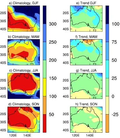
4.3.1 Seasonal stratification of trends and variability ………. 53

4.3.2 Variability of DJF rainfall and Indo-Pacific SSTs ……… 58

4.3.3 The dynamics of the observed DJF rainfall trend ……….. 64

4.4 Model rainfall variability and trend ………. 67

4.4.1 Seasonal stratification of trends and variability ………. 67

4.4.1.1 Seasonal trends ……… 67

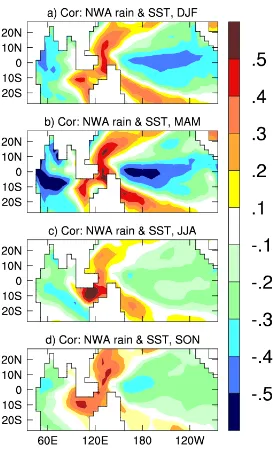
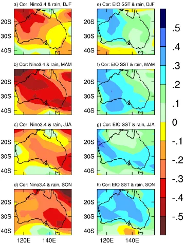
4.4.1.2 Seasonal correlation between NWA rainfall and global SST …. 69 4.4.1.3 Seasonal correlation between NWA rainfall with EIO SST and Niño3.4 ………... 71

4.4.2 Variability of DJF rainfall ……….. 71

4.4.2.1 EOF of DJF SST in the Indian Ocean ……… 71

4.4.2.2 Rainfall EOF in DJF without ENSO and IOD ……….. 75

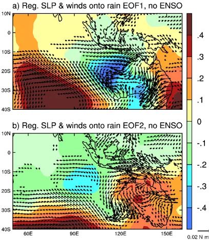
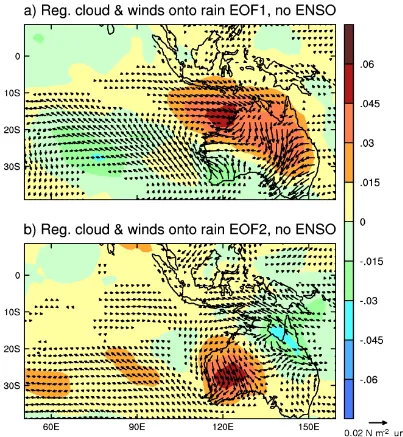
4.4.2.3 Circulation pattern associated with DJF rainfall EOFs ………. 76

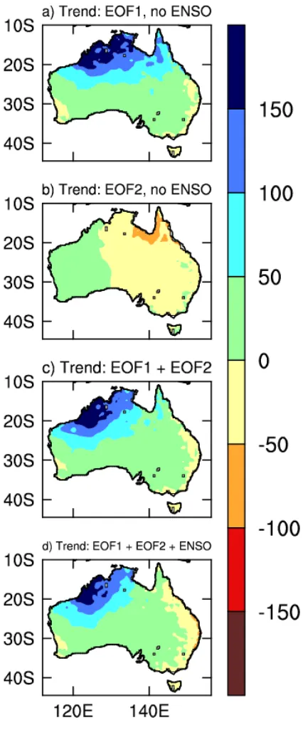
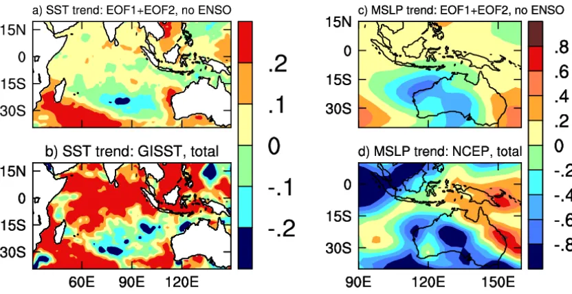
4.4.3 Dynamics of DJF model rainfall trend with increasing aerosols …… 76

4.5 Discussion ……… 80

Chapter 5: The future of Australian rainfall ………. 84

5.1 Background ………. 84

5.2 Dynamics of Tasman warming ……… 86

5.3 Dynamics of SEA rainfall variability and change ……… 90

5.3.1 Changes in summer and winter rainfall in the CSIRO model ………. 90

5.3.2 Australian rainfall teleconnction in the control climate ………. 92

5.3.2.1 Tasman Sea temperature anomalies and Australian rainfall ….. 93

5.3.2.2 The impact of ENSO ……….. 95

5.3.2.3 The impact of IOD ……… 96

5.3.2.4 The impact of the SAM ………96

5.4 Interpretation of rainfall changes ……….. 99

5.4.1 Summer rainfall change ……… 100

5.4.2 Winter rainfall change ……….. 101

5.5 Summary and discussion ……… 103

Chapter 6: Conclusions ………... 105

6.1 Indo-Pacific oceanic teleconnection ………. 105

6.2 Dynamics of NWA rainfall variability and trend ………. 106

6.3 Australian rainfall under a changing climate ……… 107

6.4 Future directions ……… 107

References ……….. 109

List of Figures ……… 123

Chapter 1: Introduction

1.1 Australia’s major climate drivers: The Three-headed dog

Australia is one of the driest continents in the world, and any factors that affect the frequency and intensity of rainfall (hence the water supply) must be explored. Australian climate variability is influenced by the El Niño-Southern Oscillation (ENSO) in the Pacific Ocean, the Indian Ocean Dipole (IOD) of the Indian Ocean (IO), and the Southern Annular Mode (SAM) of the Southern Hemisphere. The three systems can be identified from sea surface temperature (SST) and mean sea level pressure (MSLP). These three systems sometimes conspire to produce a severe impact, whereas sometimes they offset each other to produce a mild influence.

1.1.1 ENSO

The term El Niño (La Niña) refers to a periodic warming (cooling) in SST across the central and east-central equatorial Pacific Ocean (Figure 1.1, upper left). The phrase Southern Oscillation describes coherent variations of MSLP between Tahiti and Darwin (Philander, 1990). When MSLP is higher than normal in Darwin, MSLP pressure in Tahiti is lower than normal. ENSO was coined in the early 1980s in recognition of an intimate linkage between El Niño events and the Southern Oscillation, which prior to the late 1960s had been viewed as two unrelated phenomena. The global ocean–atmosphere phenomenon to which this term applies is sometimes referred to as the “ENSO cycle

.”

ENSO is associated with droughts and floods in many parts of the globe (Philander, 1990; Kiladis and Diaz, 1989). Rainfall variations over the Australian continent, especially north-eastern Australia, have been found to be significantly influenced by ENSO events (Pittock, 1975; Nicholls and Woodcock, 1981; Smith, 2004). But some El Niño events have severe impacts while some produce a mild influence. Despite great advances in ENSO theories, the underlying causes for the varying impacts are not clear.

1.1.2 The IOD

Figure 1.1: Cerberus (three-headed dog) of the Australian Climate: one head is ENSO (higher temperature in the equatorial Pacific), the second head is the IOD (higher temperature in the west and lower in the east of the IO), and the third head is the SAM (oscillating MSLP between high and midlatitudes). The ENSO anomaly pattern is obtained by regressing SST anomalies using Globe Sea Ice and Sea Surface Temperature data (GISST, Rayner et al., 1996) on an ENSO index, Niño3.4, which is defined as SST anomaly averaged over 170oW-120oW, 5oS -5oN. The IOD anomaly pattern is obtained from an empirical orthogonal function (EOF) analysis on SST anomalies, and the SAM is defined as the EOF1 of MSLP anomaly from the National Center for Environmental Predictions (NCEP) reanalysis (Kalnay et al., 1996). (Courtesy of Wenju Cai).

1.1.3 The SAM

Another driver of Australian rainfall variability, particularly over the southern part of Australia is the SAM, which is the dominant mode of variability of the Southern Hemisphere atmospheric circulation, operating on all time scales (Kidson, 1988; Thompson and Wallace, 2000). It involves opposite variations of MSLP (and geopotential height) between middle and high latitudes (Figure 1.1, lower panel). Rainfall variability at middle latitudes associated with the SAM could interfere with the influence from the Indian-Pacific system and must also be investigated.

The three systems are often referred as the “three-headed dog” (Cerberus, an ancient Greek myth) of the Australian climate (Figure 1.1). Given that climate change signals mainly project onto existing modes of variability, trends of the three modes of variability may contribute to the rainfall trend over Australia.

Figure 1.2: Total rainfall trend over the period 1950-2002 (courtesy of BMRC).

1.2 Long-term rainfall trends over Australia

populated regions rainfall decreases, particularly over eastern and southwest West Australia (SWWA). While part of the trends is simply due to multi-decadal scale variability, if these trends continue, it has important implications for water resource management across Australia.

Significant efforts have been directed to understanding the cause of some of the trends. For example, the observed rainfall decreases along the east Australia coast may reflect an increased frequency of El-Niño events in the late 20th century, which could be related to an increase in greenhouse gases; indeed, coupled atmosphere-ocean general circulation models (GCMs) forced by increasing atmospheric CO2 have simulated an El-Niño-like

warming pattern in the Pacific Ocean (e.g., Meehl and Washington, 1995; Cai and Whetton, 2000). This suggests the possibility that the observed rainfall decrease might be attributable to an El Niño-like warming pattern, and that future average rainfall might be lower over eastern Australia. To the west, rainfall over SWWA may be in part linked to a shift of the SAM towards its “positive” state, with decreased MSLP over Antarctica and increased MSLP over the SH midlatitudes (Cai et al., 2003a; Cai and Cowan, 2006). It may also be linked to multi-decadal variability of the SAM (Cai et al., 2005a), and to land-cover change (Pitman et al., 2004). One such robust feature of the Southern Hemisphere (SH) response of coupled GCMs to an increase of greenhouse gases is a strengthening (weakening) of the circumpolar (midlatitude) westerlies. (Fyfe et al., 1999; Kushner et al., 2001; Cubasch et al., 2001; Cai et al., 2003a). However, as with interannual rainfall variations, the relative importance of the contributions from the trends in the three systems is not clear.

As shown in Fig. 1.2, there has been an overall positive trend in rainfall over North West Australia (NWA). In an environment in which decadal-scale droughts have plagued most of the country, and the long-term rainfall over southern Australia is projected to decrease further, continued upward trends in NWA rainfall may provide a source of future water resources in NWA. However, the dynamics governing the rainfall increase is not fully understood. There is evidence that the upward trend in the SAM index has caused considerable changes in ocean circulation (Cai et al., 2005b). Will this in turn, modulate the rainfall response?

1.3 Foci of the present project

Based on an extensive literature review, focus will be placed on three areas:

ENSO signals into the IO via oceanic teleconnection. We will focus on the decadal-scale variability of the process and the impacts on Australian rainfall.

2) Dynamics of the NWA rainfall trends. This is an area in which our knowledge is virtually void, but the robustness of the water abundance is very important because it could provide a resource to alleviate Australia’s water shortage.

3) The future of Australian rainfall, in terms of the response of climate drivers and their teleconnection with Australian rainfall to climate change forcing. This will take into account that the net rainfall change in the future will be a consequence of both super-imposing effects and offsetting influences by the three climate engines.

In the following sections, current status of the research in each of the areas is described; the knowledge gaps in which contribution can be made are identified.

1.3.1 Indo-Pacific transmission and impact on Australian rainfall

This area concerns the tropical pathway of the Indo-Pacific exchange. Statistical analyses of historical SST records (e.g., Pan and Oort, 1983, 1990; Kiladis and Diaz, 1989; Hastenrath et al., 1993; Kawamura, 1994; Tourre and White, 1995; Lanzante, 1996; Nicholson, 1997; Harrison and Larkin, 1998; Klein et al., 1999; Enfield and Mestas-Nun˜ez, 1999; Larkin and Harrison, 2001) have indicated that the surface conditions of the IO are related to ENSO events. Some of these studies reported that the strongest SST anomalies in IO typically appear several months after the mature phase of the ENSO signal in the central equatorial Pacific. But there are few studies dealing with ways in which ENSO signals are transmitted from the Pacific into the IO. The location where the Pacific Ocean signals end up, however, affects variability in the IO, which in turn influences rainfall variability over south-eastern Australia. The objective is to address this issue by utilizing available oceanic reanalysis data and reconstructed sea level data, which is a surrogate for oceanic heat content, recently made available.

1.3.1.1 Current knowledge

SST anomalies in the EIO are dominated by IOD events in the IO. This discovery has raised a number of new questions about its generation and possible interactions with other climate phenomena such as ENSO. An IOD (Saji et al., 1999; Webster et al., 1999) episode usually begins with anomalous cooling in the tropical EIO during May–June, when enhanced surface easterlies generate an anomalously shallow thermocline, enhanced latent heat flux, and upwelling off the Sumatra–Java coast. The cold anomaly usually peaks in September–October, by which time the western IO has warmed as a result of increased insolation, reduced evaporation, and deepened thermocline. The demise of an IOD often occurs soon after the Australian summer monsoon commences in December, when the mean winds become westerly in the equatorial EIO. The induced easterly anomalies then act to reduce the wind speed. Reduced latent heat flux alone with increased surface shortwave radiation acts to warm the EIO, yielding basin-scale warm anomalies. This seasonality in the evolution of the IOD is often referred to as the seasonal phase-locking feature. Development of an IOD, typically, but not always, accompanies development of an El Niño in the Pacific Ocean.

Figure 1.3: Relationship between winter rainfall anomalies over MDB region and winter EIO SST anomalies (averaged over an area bounded by 5oS-10oS and 100oE-110oE), and between winter rainfall anomalies over MDB region and winter Niño3.4 index. The figure shows that for MDB region, the winter rainfall is influenced more by SST in the EIO.

The Indo-Pacific linkage in terms of tropical oceanic teleconnection is via the Indonesian Throughflow (Meyers, 1996; Potemra, 2001), which is a system of surface currents flowing from the Pacific to the IO through the Indonesian seas. It is the only flow

Eastern Indian Ocean SST

between the ocean basins at low latitudes and, consequently, plays an important role in the meridional transport of heat in the climate system, all the more so since this transport originates from the warm-pool of the Pacific Ocean and enters into the colder waters of the South Equatorial Current of the IO.

The variability of Indonesian Throughflow and its linkage with ENSO has long been a subject of great interest. Wyrki (1987) compared the sea level measured at Davao (Philippines) and Darwin (Australia). He noticed that while there are variations of sea level at both ends of the throughflow, the difference between these levels remains almost constant. According to Barnett (1983), the convergence of surface winds over Indonesia is subject to strong interannual variations in its intensity and location because of the coupling of the trade winds over the Pacific with monsoons over the IO. A strong convergence of the wind field is associated with a high state of the Southern Oscillation Index, i.e. a La Niña phase, sea level rises both in the EIO and in the western Pacific Ocean. During a low state of Southern Oscillation Index, i.e., an El Niño, winds are divergent over Indonesia, and sea level drops on both sides of the Indonesian archipelago. These characteristics of the wind field imply that the difference of sea level between the western Pacific and the EIO is only weakly affected by the principal wind patterns associated with ENSO. Wyrtki attributes the slow interannual variations of the sea level difference between Davao and Darwin to fluctuations in the wind field which are not associated with the Southern Oscillation, or may be due to uncertainties in the sea level records themselves.

However, Clarke and Liu (1994) suggest that the volume transport of throughflow is expected to vary during ENSO, with a larger than normal transport during La Niña, when strong easterlies along the equatorial Pacific Ocean build up high sea level in the western Pacific. In theory, the Pacific Ocean signal is regarded to be transmitted to the north-western coast of Australia and influences the throughflow by geostrophy by the difference in sea level between the Indian and Pacific Ocean. Clark and Liu argue that Wyrtki (1987) did not use a sea level difference that is representative of the relevant pressure gradient due to the choice of Darwin to representing the IO. Darwin is, in fact, representative of the Pacific Ocean during ENSO cycle. The difference between Davao and the southern coast of Java is a more appropriate gradient to measure the Pacific to IO pressure gradient. Meyers (1996) studied the observed data from the expendable bathythermograph (XBT) line between Fremantle and Sumatra. He concluded that the ENSO signal that appears on the northwestern coast of Australia is forced by winds in the equatorial Pacific. He also proposed that thermocline variations along the Java coast are driven by zonal wind: easterly wind anomalies over the equatorial IO are associated with shallow thermocline and colder waters.

westward as a Rossby wave. Upon impinging on the western boundary, it moves equatorward along the Kelvin-Munk ray-path proposed by Godfrey (1975), and reflects as an equatorial Kelvin wave. As the reflected Kelvin wave propagates eastward, it impinges on the Australasian continent and moves poleward along the WA coast as a coastally-trapped wave, radiating Rossby waves into the south IO (Wijffels and Meyers, 2004). Along the above path, the NP anomaly reaches the central WA coast some 9 months later. On-route to the WA coast the anomaly is reinforced by evolving winds associated with ENSO.

Coupled climate models have largely been unable to simulate the transmission process of ENSO signals from the Pacific into the IO (Cai et al., 2005d). The underlying cause is not clear yet. The likelihood that the process is non-stationary needs to be investigated.

1.3.1.2 Scope

While much of the focus of recent research has been on the ENSO linkage to the IO on interannual time scales, analysis so far has largely been limited to the period since 1980 due to limitations of available data,. Multidecadal variability of the linkage has not been explored. Since the mid-1970s, climate has been known to shift to a state considerably different from that prior to mid-1970s (IPCC, 2007; Hartmann, 1994; Hurrell and Trenberth, 1996). Our hypothesis is that associated with this climate shift, the statistical relationship between variability in the Indian and the Pacific Ocean may undergo a significant change. Understanding the physical processes responsible for these changes is crucial for realistic simulations of the Indo-Pacific dynamics in coupled climate models, for assessing their climate impacts, and for detection of climate change signals. Recent reconstructed oceanic analysis will enable such a study to proceed.

1.3.2 Dynamics of NWA rainfall variability and change

Figure 1.2 shows that, in sharp contrast to significant drying trends in other regions of the country, there has been an overall positive trend in rainfall over NWA. The observed annual increase is approximately 50% of the climatological value (Fig. 1.4). Policy makers are considering a northern development, to take advantage of the water aboundance. However, a detailed knowledge of climate processes governing its stability under a changing climate is still lacking. We will examine the dynamics of observed rainfall variability and trends, benchmark the performance of available climate models focusing on role of anthropogenic forcing in driving the observed trend, and identify model deficiencies so as to improve projection of future NWA rainfall changes.

1.3.2.1 Current knowledge

increasing atmospheric CO2 have simulated an El-Niño-like warming pattern in the

Pacific Ocean (e.g., Meehl and Washington, 1995; Cai and Whetton, 2000). This suggests the possibility that the observed rainfall decrease might be attributable to an El Niño-like warming pattern, and that future average rainfall might be lower over eastern Australia. To the west, rainfall over SWWA may be in part linked to a shift of the SAM towards its “positive” state, with decreased MSLP over Antarctica and increased MSLP over the SH midlatitudes (Cai et al., 2003a; Cai and Cowan, 2006). It may also be linked to multi-decadal variability of the SAM (Cai et al., 2005a), and to land-cover change (Pitman et al., 2004). One such robust feature of the SH response of coupled GCMs to an increase of greenhouse gases is a strengthening (weakening) of the circumpolar (midlatitude) westerlies. (Fyfe et al., 1999; Cubasch et al., 2001; Cai et al., 2003a).

Figure 1.4: Time series of summer NWA rainfall in terms of percentage of climatology. NWA is defined as the area of 110oE-130oE, 10oS-20oS.

By contrast, there is relatively little understanding of the dynamics of NWA rainfall variability and trends. Two recent studies have shed some light. Wardle and Smith (2004) hypothesized that during the latter half of the 20th century, the observed increase in temperature gradient between Australia and neighbouring oceans drove a stronger monsoonal circulation. They found that by artificially altering this contrast through a change to the land albedo in a model, they could simulate an increase in rainfall over the entire continent, with stronger totals over the north. Their experiment also resulted in a

temperature response similar to the observed. They concluded that the temperature changes were possibly leading to a strengthening of the monsoon and that this was the cause of the increased rainfall. However, the prescribed changes were much larger than could be justified based on current knowledge, so the authors left the cause of the land-ocean temperature contrast as an open question.

An alternative explanation for the increased northwest rainfall was provided by Rotstayn et al. (2007) who, by using simulations from a low resolution coupled GCM, demonstrated that including (excluding) anthropogenic aerosol changes in 20th century gives increasing (decreasing) rainfall and cloudiness over Australia during 1951–1996. Rotstayn et al. (2007) showed that the pattern of increasing rainfall when aerosols are included is strongest over NWA, in agreement with the observed trends. The strong impact of aerosols is predominantly due to the massive Asian aerosol haze, as confirmed by a sensitivity test in which only Asian anthropogenic aerosols are included. The Asian haze alters the north-south temperature and pressure gradients over the tropical IO in the model, thereby increasing the tendency of monsoonal winds to flow towards Australia.

The argument of an impact from aerosols seems to be supported by the fact that transient climate model simulations forced only by increased greenhouse gases, without the inclusion of aerosol forcing, have generally not reproduced the observed rainfall increase over northwestern and central Australia. Whetton et al. (1996) compared rainfall changes in five enhanced greenhouse climate simulations that used coupled GCMs, and five that used atmospheric GCMs with mixed-layer ocean models. The coupled experiments mostly gave a decrease in summertime rainfall over northwestern and central Australia, whereas the mixed-layer experiments mostly gave an increase (in better agreement with the observed 20th century trends). They attribute the difference to the coupled model feature that a stronger overall warming occurs in the northern Hemisphere than in the SH, which is expected to lead to a similar hemispheric imbalance in rainfall (Murphy and Mitchell, 1995). The hemispheric asymmetry in warming is due to the greater proportion of ocean in the SH, and much greater thermal inertia of the SH oceans causing a delayed warming relative to the northern Hemisphere (Stouffer et al., 1989, Cai et al., 2003a).

1.3.2.2 Scope

1.3.3 The future of Australian rainfall

Within the Indo-Pacific system, the subtropical pathway, i.e., through the EAC, for transmission of Pacific signals has not been well studied. Observational evidence suggests the strength of the sub-tropical exchange has been changing with strong impacts on climate and marine ecosystem. The changing strength means that the properties of the Pacific Ocean circulation, such as the EAC, its separation location, and the inflow/outflow partition have been changing. Simultaneously, Southern Hemisphere atmospheric circulation has been marked by substantial trends. We will explore the dynamics of their possible linkage, and the combined impact, in particular, the likelihood of a feedback into the atmosphere as a consequence of the changing EAC that provides an influence on future Australian rainfall.

1.3.3.1 Current knowledge

Variations of the SH atmospheric circulation have been shown to be organized into a number of well-defined spatial patterns (Kidson, 1999). The most prominent of these low-frequency circulation patterns is characterized by a predominantly zonally-symmetric pattern, a see-saw meridional variation in the zonal wind strength between 40oS and 60oS, and an equivalent barotropic structure in the vertical (Kidson, 1988a; Shiotani, 1990; Hartmann and Lo, 1998; Thompson and Wallace, 2000; Rashid and Simmonds, 2004). It has variously been called the Antarctic Oscillation (Gong and Wang, 1999), and the SAM (Limpasuvan and Hartmann, 1999). It will be referred to as the SAM throughout this thesis.

The SAM is the leading mode of Southern Hemisphere circulation variability. Thompson and Wallace (2000) revealed the SAM as the leading EOF in many atmospheric fields, including MSLP, geopotential height, surface temperature, and zonal wind. The oscillations exist year-round in the troposphere, but it amplifies with height upward into the stratosphere during certain times of the year or “active seasons.” The SAM contributes to a significant proportion of SH climate variability from high-frequency (Baldwin, 2001) through to very low-frequency time scales (Kidson, 1999). Modeling studies indicate that the SAM is also likely to drive the large-scale variability of the Southern Ocean (Hall and Visbeck, 2002).

As shown in Fig. 1.2, SWWA has experienced a substantial drying trend with a winter rainfall decrease of some 20% (IOCI, 2002). The decline manifests itself as a reduction in high-intensity winter rainfall events, and is accompanied by an upward trend of the SAM (Thompson et al., 2000; Marshall, 2003; Marshall et al., 2004) with increasing MSLP in the midlatitudes. The cause of the upward trend of the SAM is a contentious issue. Observational (Thompson and Solomon, 2002) and other modelling studies (Sexton, 2001; Gillett and Thompson, 2003) indicate that it is attributable to ozone depletion over the past decades. Climate models produce increasing midlatitude MSLP under increasing atmospheric CO2 incorporated in an upward trend of the SAM (Fyfe at

SWWA decreases in the transient period while CO2 increases (Cai et al., 2003a). A

recent study (Cai and Cowan, 2006) indicates that at least 50% of the observed SWWA

Figure 1.5: Wind-drive ocean circulation (in Sv, 1 Sv = 10-6 m3 s-1) calculated using NCEP winds, a) over the period of 1948-1967, and b) over the period of 1981-2000. The comparison shows a stronger EAC flow passing the Tasman Sea, consistent with what is predicted by couple climate models.

rainfall reduction is driven by anthropogenic forcing. Although such a decrease in midlatitude rainfall is consistent with a reduction in extratropical SH cyclones, one would expect that a similar reduction in rainfall over the southeastern Australia, where however, the model rainfall reduction is less than that over SWWA. We hypothesize that changing ocean current as a result of wind changes associated the SAM is a potential process accounting for the different rainfall response between SWWA and southeast Australia. Specifically, an intensifying EAC will transport warmer water south, which promotes convection and rainfall, providing a mechanism offsetting the rainfall reduction associated with rising MSLP incorporated in the upward trend of the SAM.

There are little ocean observations available to examine the oceanic impacts of the atmosphere circulation trends, but it can be assessed partially through surface wind changes. We will use the trends in surface winds to estimate oceanic circulation change and assess the importance of ozone depletion in driving the change. Figure 1.5 shows the wind-driven barotropic ocean circulation (in Sv, 1 Sv = 10-6 m3 s-1), determined with

a), Average over 1951-1970

Godfrey’s Island Rule model (Godfrey, 1989) forced with NCEP reanalysis data (Kalnay et al., 1996). The results indicate that over the past decades the entire Indo-Pacific Southern Ocean circulation has changed significantly, with an intensifying southern mid-latitude ocean circulation including the EAC. All climate models consistently produce an upward trend of the SAM. We will examine its influence on ocean circulation change, and its impact on Australian rainfall.

1.3.3.2 Scope

Attention will focus on how the subtropical oceanic circulation pathway has been changing over the past 50 years, and identify the level of impact it exerts. The issue of how the Southern pathway may respond to anthropogenic forcing. There is virtually no ocean observation in the South Pacific which covers a meaningfully long period. However, there are sufficient atmospheric observations and reanalysis, from which aspects of the ocean circulation can be derived. The impact of the changing ocean circulation on Australia rainfall will be assessed, together with the impacts from the trends of other climate drivers. Coupled climate model simulations under climate change forcing will provide the needed data sources.

1.4 Summary

We will focus on the three key areas in which a contribution can be made to better understand the dynamics governing rainfall variability and changes in Australia. Significant progress in our knowledge is needed in order to enhance our projection capability of future rainfall and hence water resources. The key questions we pose are:

o Is there a varying relationship between variability in the Pacific Ocean (ENSO) and in the IO, and how it contributes to the observed rainfall variations and trends? This and the related issues are addressed in Chapter 3.

o What are the dynamics governing variability and trends of rainfall over NWA? Is it really caused by anthropogenic aerosol forcing? We explore these questions in Chapter 4.

o What is the future of Australian rainfall, taking into account of possible changes in climate drivers and in ocean-atmosphere circulation? Chapter 5 provides a consensus projection and an interpretation.

The project has so far contributed to many publications, some are listed below. These are:

1. Shi, G., J. Ribbe, W. J. Cai, and T. Cowan (2008a), An interpretation of Australian summer and winter rainfall projection. Geophysical Research Letters, 35, L02702,.doi:10.1029/2007GL032436.

2. Shi, G., W. J. Cai, T. Cowan, J. Ribbe, L. Rotstayn (2), and M. Dix (2008b), Variability and trend of the northwest Western Australia Rainfall: observations and coupled climate modeling. Journal of Climate, 21, 2938–2959

4. Cai, W. J., T. Cowan, M. Dix, L. Rotstayn, J. Ribbe, G. Shi, and S. Wijffels (2007) Anthropogenic aerosol forcing and the structure of temperature trends in the southern Indian Ocean. Geophysical Research Letters, 34, L14611, doi:10.1029/2007GL030380.

5. Cai, W. J., Meyers, G. A., and Shi, G. (2005). Transmissions of ENSO signal to the Indian Ocean. Geophysical Research Letters, 32 (5): 5616, doi:10.1029/2004GL021736.

Chapter 2: Data and Methodologies

To elucidate a physical process, multiple data sets and a combined deployment of several analytical techniques are required. Detailed rationales for a specific combination of data and methods adopted will be provided in Chapters 3 to 5, as we address specific issues identified in Chapter 1. Here, we outline the details of the models, data and methodologies used. These have been applied by Shi et al. (2007), Shi et al. (2008a, 2008b).

2.1 Data

2.1.1 Observations and reanalyses

The observed rainfall data are from the Australian BMRC and updated version of GISST datasets (Rayner et al., 1996). Although these two datasets cover a period from late 19th century to 2006, we focus on the 50 year period from 1951-2000. To understand the circulation associated with rainfall patterns, MSLP and surface winds data, and other fields from the NCEP reanalysis are used (Kalnay et al., 1996).

The ocean thermal analysis is the operational subsurface temperature reanalysis from the BMRC (Meyers et al., 1991; Smith, 1995a, 1995b), which is an optimal interpolation on a 1oC latitude by 2oC longitude grid at 14 depth levels, throughout the Indo-Pacific basin. It is based primarily on XBT profiles and time-series from the Tropical Atmosphere Ocean buoy array (McPhaden et al., 1998), and covers a 20-year period since 1980. The data in the Pacific Ocean domain has been used in numerous studies (Meinen and McPhaden, 2000; Cai et al., 2004; Kessler, 2002). The relationship of oceanic variability to the wind field is documented with data from the NCEP reanalysis (Kalnay et al., 1996).

We utilize the newly available reanalysis of the Simple Ocean Data Assimilation Parallel Ocean Programme (SODA-POP) version 1.4.2 (Carton and Giese, 2006). The new model product uses the European Center for Medium Range Forecasts ERA-40 atmospheric reanalysis winds. It has a spatial resolution of 0.5oC latitude by 0.5oC longitude grid, and covers a period from 1958 to 2001. Both the SODA-POP and BMRC reanalyses independently incorporated Expendable Bathythermograph profiles and time-series from the Tropical Atmosphere Ocean buoy array (McPhaden et al., 1998). We find that there are remarkable differences in the transmission between the pre- and post-1980 periods. Cai et al. (2005c) discussed the post-1980 transmission. Our analysis focuses on the pre-1980 period.

2.1.2 Climate models and outputs

The CSIRO Mark 3.0 climate modelhas been significantly improved relative to the Mark 3a model (Gordon et al., 2002). It is run without the use of flux adjustments. The horizontal resolution of the atmospheric model is spectral T63 (approximately 1.875° latitude, 1.875° longitude) with 18 vertical levels (hybrid sigma-pressure vertical coordinate). The atmospheric model includes a comprehensive cloud microphysical parameterization (Rotstayn et al., 2000) and a convection parameterization based on that used in the Hadley Centre model (Gregory and Rowntree, 1990). This convection parameterization is linked to the cloud microphysics scheme via the detrainment of liquid and frozen water at the cloud top. Atmospheric moisture advection (vapor, liquid, and frozen) is carried out by the semi-Lagrangian method (McGregor, 1993). A simple treatment of the direct radiative effect of sulphate entails a perturbation of the surface Albedo (Mitchell et al., 1995). The land surface scheme (six layers of moisture and temperature) with a vegetation canopy (Kowalczyk et al., 1991, 1994) includes a three-layer snow model. Multiple soil types and vegetation types are included.

The Mk3.0 ocean module is based upon the Modular Ocean Model (MOM2.2) version of the Geophysical Fluid Dynamics Laboratory model. The oceanic component has a horizontal resolution matching that of the atmospheric model’s grid in the east–west direction and twice that in the north–south direction. Thus the grid spacing is approximately 0.9375° latitude × 1.875° longitude. Because there are two ocean grid points per atmospheric grid point in the meridional direction, the atmosphere model and ocean model subcomponents have identical land–sea masks. There are 31 vertical levels and the level spacing gradually increases from 10 m at the surface to 400 m in the deep ocean. A parameterization of mixing of tracers based on the formation of Griffies et al. (1998) and Griffies (1998) is included.

In this thesis, the analysis of outputs from a control simulation and four climate change experiments is discussed. The control simulation will be used to examine the relationship of Australian rainfall with the three engines of the Australia climate and with the Tasman Sea Surface Temperature (SST). For this purpose anomalies are obtained and referenced to a 300 year climatology. Previous studies have described the simulation of the ENSO and the IOD in this version of the model (Cai et al., 2003b; Cai et al., 2005a). Four climate change experiments follow the Intergovernmental Panel on Climate Change (IPCC) A2 (two experiments), A1B, and B1 scenarios that all incorporate CO2 forcing,

the direct effect of sulfate aerosols (direct effect only), and stratospheric ozone depletion. Each of the four experiments starts from a different time of the control experiment and together they provide an ensemble strategy. These data are used to study the impact of the Tasman Sea warming on Australia rainfall and the future Australia rainfall changes (see Chapter 5).

while the ocean has 21 vertical levels. A detailed description is provided by Rotstayn et al. (2007). The low-resolution allows fast integration of experiments with the comprehensive aerosol scheme, all covering the period 1871 to 2000. The aerosol species treated interactively are sulfate, particulate organic matter (POM), black carbon (BC), mineral dust and sea salt. As well as the direct effects of these aerosols on shortwave radiation, the indirect effects of sulfate, POM and sea salt on liquid-water clouds are included in the model. Historical emission inventories are used for sulfur. POM and BC derived from the burning of fossil fuels and biomass. Other forcings included are those due to changes in long-lived greenhouse gases, ozone, volcanic aerosol and solar variations (but changes in land cover are omitted). The ensemble consists of eight runs with all of these forcings (ALL ensemble). A further eight runs with all forcings, except those related to anthropogenic aerosols (AXA ensemble), differ only from the ALL ensemble in that the anthropogenic emissions of sulfur, POM and BC were fixed at their 1870 levels.

The analysis of these experiments is presented in Chapter 4 and focuses upon the causes of the NWA rainfall trends. Outputs from a multicentury (300 years) control experiment without climate change forcing are also used to examine if the model reproduces the rainfall teleconnection with large scale circulation fields. Outputs from the ALL ensemble are projected onto modes of variability in the control experiment.

The CSIRO Mk3.5 climate model has the same resolution as that of Mk3.0, but is improved in many aspects. During the course of my Ph. candidature, the improved model is run without climate change forcing, i.e., in the control climate setting. One of the most important improvements is that it overcomes a problem associated with the timing of signal transmission from the Pacific to the IO. We use the output to examine the robustness of multidecadal variability in the transmission. We use the results of a multi-century control experiment with this model. The new version simulates a more realistic transmission process, although it still suffers from the common cold tongue bias, i.e., the equatorial Pacific cold tongue extends too far west. The ENSO frequency is reasonably simulated as reported earlier (Cai et al., 2003b) but the amplitude is too large. Despite these deficiencies the model produces multidecadal variations in the transmission similar to the observed (see Chapter 3).

2.2 Methodologies

Besides the commonly used correlation and regression analyse, we also apply EOF analysis, complex EOF (CEOF), and projections onto modes of variability. These and others are described below. We also point out Chapters where these methodologies are used.

2.2.1 EOF (Empirical Orthogonal Function)

identifies patterns of variability, and if variance of an identified pattern is large enough, there is often an identifiable physical mechanism that operates to generate the pattern.

A main feature of an EOF analysis is that it identifies correlations inherent in the data by re-organizing the original data into individual clusters in space or time. This can effectively compress a large number of spatially and temporally correlated values into both space and time components, while also splitting the temporal variance of the data series into a set of orthogonal spatial modes (also called eigenvectors) that explain a large proportion of the measured variance (Peixoto and Oort, 1992). This type of analysis has been used in climatological work for many years (e.g. in particular Lorenz since 1956) and its usage has steadily increased. It is a convenient method for analysing climatological fields (e.g., North et al., 1982).

Consider the value of a field at N spatial locations which have M monthly observations (t). Thus, the field at any one time form a spatial map of, for example, SSTs. Each map in the time series can be written mathematically as a vector of length N, producing,

)

...

,

(

_{m1 m2 mN}

m

z

z

z

z

=

where m represents the time instant in the series of observations, e.g., m = 1, 2, …, M. As a result, a M x N matrix containing the full time series of spatial elements is easily formed,

























=

MN M M N N

z

z

z

z

z

z

z

z

z

z

L

M

M

M

M

L

L

2 1 2 22 21 1 12 11

The M rows represent the spatial maps at each time step and the N columns are the time histories at individual spatial locations. Therefore, an individual element of the matrix Z represents the SST at time m and spatial location n. To carry out the EOF analysis (i.e., find the orthogonal spatial modes), we need to maximize the expression,

(

)

∑

= ⋅ − M m n m v z M 1 2 1 1 (E1)

for each individual spatial location (i.e., n = 1, 2, …, N) subject to the conditions,

i n if 0 i n if 1 { ≠ = = = ⋅ i T n i

n v v v

v (E2)

where vn is the orthonormal vector that optimally represents the original data vector, zm.

(

)

(

)

n T n n T T n n

m v zz v v Cv

M v

z

M −

∑

⋅ = −1 =

1 1

1 2

where C would normally symbolize the covariance matrix (Peixoto and Oort, 1992). However, if one is comparing different model output fields, the correlation matrix (C) should be used as it will provide equal weighting of the different variables analysed and a sensible comparison of results between the model fields (von Storch and Zwiers, 1999).

The correlation matrix of the SST anomalies is defined by:

)

(

)

(

Z

Var

Z

Var

Cov

C

T

=

This is an M x M real symmetric matrix where

Z Z M Cov T 1 1 − =

The maximization of [vT_n C V_n], subject to the condition (E2), establishes a variational problem which leads to eigenvalue problems or characteristic value problems. However the problem can be solved by,

n n

n

v

Cv

=

λ

where

λ

_n is the eigenvalue associated with the characteristic eigenvector (vn) of the

correlation matrix, C. Each of the associated eigenvalues (

λ

_n) identifies the fraction of the total data variance explained by the eigenvector, which is given by,

∑

= N 1 i i n λ λ

The eigenvalues are ordered to decrease with successive modes such that the first eigenvector and its associated eigenvalue explain the largest portion of the total variance, while the second eigenvector and its associated eigenvalue explain the second largest portion of the total variance and so forth (von Storch and Zwierss, 1999). The total number of spatial modes generated in an EOF analysis is equal to the smallest dimension of the original data matrix.

m n

mn

v

z

w

=

These weighting coefficients represent how well the mode vn describes the observation

z_n (Peixoto and Oort, 1992). Thus, theoretically any observation of SST (zn) can be

expressed as the linear combination of the eigenvectors vn,

n N

n mn

m

w

v

z

=

∑

=1

This can be written in matrix notation as,

ZV

W

=

The elements of the columns of W [w1n, w2n, …,wMn] are the dimensional time

coefficients associated with the eigenvector vn. Thus, it is the eigenvector’s

corresponding time series that displays the temporal behaviour of the mode. These time components are commonly referred to as expansion coefficients. It is also important to note that these column vectors [w1n, w2n, …,wMn] are mutually orthogonal (Peixoto and

Oort, 1992).

Although this method of analysis is purely mathematical, the larger the variance explained by the dominant modes of a system, the more likely they are to be physically meaningful (Peixoto and Oort, 1992). The number of important spatial modes identified by an EOF analysis is determined based on the eigenvector spectrum and, for example, the mode degeneracy (e.g., North et al., 1982). In most cases, the majority of the data variance can nomally be explained by only the first few EOFs (von Storch and Zwiers, 1999).

2.2.2 CEOFs and Statistical Significance of Monthly and Filtered Time Series

An EOF analysis allows identification of a stationary pattern. In Chapter 3 we will be discussing the propagation of the Indo-Pacific signals into the IO, and we used filtered data. This propagation can be described by lag correlation and regression, or by complex EOF (CEOF). All these methods are used. Here, we use a routine described by Barnett (1983). Time sequence data at each spatial location is Hilbert-transformed to obtain a complex time sequence, the real part being the input data and the imaginary part representing signals that are identified to be related with the real part but are 90o out of phase. The complex eigenvectors and complex principal components are then found by singular value decomposition of the matrix. These procedure are well developed, below we discuss the statistical significance based on monthly and filtered time series.

(2) The variables being considered are all jointly normally distributed, being part of respective populations that have underlying means, variances, and covariances. (3) The data sets used are unbiased samples of these populations.

In an analysis of climate data, there may be problems with each of these assumptions. Long-period variations such as the Interdecadal Pacific Oscillation may affect data sets of length < 20 years or so, and the normality of variables on these timescales is uncertain. The representativeness of samples is perhaps the least questionable of these assumptions, but this is also sensitive to processes on timescales longer than the length of the record. Given these uncertainties, a statistical analysis of uncertainties of climate data sets is probably only useful as a guide, and though it provides answers, these should not be expected to constitute firm conclusions about significance. Nevertheless, we pursue it here.

The relationship between the time series of any two observed variables x(t) and y(t) (such as the SST at two particular grid points) is measured by covariance between them and, as computed from the data, is denoted vxy. However, this computed covariance is just an

estimate from the sample of data available of the underlying covariance µxy of the

assumed population of SSTs at these two grid points. It is this latter quantity that we are trying determine. How good is the estimate? A measure of this is given by the variance

s2_xy (or standard error sxy ) of vxy defined by

s

xy

2

= E(vxy – µxy)2 = E (vxy)2 - µ

2

xy , (A1)

where E denotes the expected value, and µxy = E (vxy). We do not know µxybut must

estimate it vxy, so that

s

xy

2

= E(

v

_xy)2 –

v

2_xy (A2) If x and y are complex time series,

v

_xy = cov(x,y) =

N

1

]

)

(

][

)

(

[

x

t

x

y

t

_i

y

N i

i

−

−

∑

=1

,

x

=

N

1

)

(

∑

= N i i

t

x

1 (A3)

s

xy 2

=

E

{

[

x

(

t

)

x

][

y

(

t

)

y

]

*

[

x

(

t

)

x

][

y

(

t

)

y

]

*

}

N

i j j

N i

N j

i

−

−

×

−

−

∑∑

=1 =1 2

1

-

E

[(

v

_xy

)]

2 (A4)

where an asterisk denotes a complex conjugate. covariances such as vxy may be complex,

with means µx and µy, variances σ

2

x and σ

2

y, and (complex) correlation coefficient rxy.

Then (A4) reduces to (Papoulis,, 1965; Davis, 1976)

s

xy 2 =

N

y x 2 2

σ

σ

{1 +

r

_xy 2+

[Re(

(

)

(

))

(

)

2

]

2 1 1

j

r

j

r

j

r

_{yy xy}

N j xx

+

∑

− =

} (A5)

where N is assumed to odd for convenience, Re denotes real part, and rxx(j) denotes the

time-lagged correlation coefficient for x with lag j

∆

t

, where

∆

t

is the time interval between samples. Quantities on the right-hand side of (A5) must be estimated from their sample values, taking

σ

_x2 = v_xx,

σ

2_y =v_yy, r_xy=v_xy/(v_xxv_yy)1/2, etc. If

∆

t

was significantly large, so that the values of x(t_i), y(t_i) were all independent from each other, the lag correlation terms would all vanish. We would have N independent sample pairs, or “degrees of freedom,” so that in this case,

s

xy 2 =

N

y x 2 2

σ

σ

[1+

r

_xy 2]. (A6)

Equation (A5) may then be used to define an effective number of degrees of freedom N∗

in (A6) (Davis, 1976)

N∗=

∑

=−

+

+

+

+

2 1 1 2 2 2

2

1

1

N

j xx yy xy xy xy

j

r

j

r

j

r

r

r

N

]}

)

(

))

(

)

(

[Re(

{

)

(

(A7)

Taking vxy+ / -sxy gives an estimate of µxy , with error bars the width of the standard error.

To test the significance of CEOFs, we follow the procedure described by North et al. (1982) and consider an array of m grid points at each of which there is an observed series of values of a variable x at N times. These times are simultaneous and evenly spaced with interval

∆

t

. Hence we have an array of data xj(tk), j = 1, …m and k=1, …N. From these

we may obtain CEOF by taking the Hilbert transform hj(tk) of the time series at each grid

point and then defining the complex time series

X_j(t_k) = x_j(t_k) + ih_j(t_k). (A8)

We then define the m

×

m matrix of complex covariances Sij = cov (Xi, Xj) by (A3). The

spatial structure of the CEOFs is then given by the eigenvalue equation

),

(

)

(

j

l

f

i

f

S

m j

ij α

=

α α

∑

=1

where Sij is Hermitian, so that the eigenvalues lα are all real and positive and the

eigenvectors f α are complex. These form a linearly independent set, with α = 1, …m.

In accordance with the assumptions mentioned above the background population of which the xirepresent a sample are assumed to be statistically and have underlying values

of the covariances at the m grid locations that may be represented by vij. From these exact

(but unknown) covariances the exact eigenvalues λαand eigenvectors

φ

α (i) are given by

),

(

)

(

j

i

f

v

m j

ij α

=

λ

α

φ

α

∑

=1

α

, i = 1, …m. (A10)

One may expect that the deviations of the sample covariances Sijfrom the actual

covariances vij will be of the order of the standard errors of the Sij, so that we my write

S

_ij =

v

_ij +

ε

V

_ij , (A11)

where ε is a small parameter of order (2/N*)1/2 and Vijis of the order of

V

_ij = [(

v

_ii

v

_jj +

v

_ij

v

*_ij)/2]1/2 (A12) where N* is given by (A7) with Xi and Xj in the place of x and y. In practice, we take a

mean value for N* over all pairs Xi, Xj. for values of the vij we use the sample values Sij.

One may then use a standard perturbation expansion of the form

f

α =

φ

α(i) +

ε

f

α (i)

) (1

+ …, (A13)

l

α =

λ

α+

ε

l

) (1

α + …, (A14)

to obtain the first-order deviations due to the perturbations in the vij. These give (North et

al., 1982)

l_α(1) = *

(

i

)

V

_ij

(

j

)

m i

m

j

φ

α

φ

α

∑∑

=1 =1

, (A15a)

λ

α

) (1

= *

(

i

)

v

_ij

(

j

)

m i

m j

φ

φ

_{α α}

∑∑

=1 =1

, (A15b)

)

(

i

m

a

f

φ

_β

β α

α

∑

β

=

=

1

a

αβ=

λ

λ

φ

φ

β α α β

−

∑ ∑

= = m i m

j

i

V

ij

j

1 1

(

)

(

)

*

. (A16b)

Since Vij is of the same order as vij ( Vii

≈

vii), from (A15) we have _α (

λ

_α

) 1 (

O

l

= ), so that the magnitude of the uncertainty in the eigenvalue

δ

λ

_α is approximately

λ

α

δ

=

ε

λ

_α(1)

≈

λ

_α

2 / 1 * 2    

N . (A17)

If one eigenvalue is much larger than the others, the form of (A15) indicates that (A17)

may be an overestimate. In these cases, sample computed values for

l

(₁1) using (A15) generally give much smaller values than those from (A17). Clearly, this criterion should be taken as a guide and these uncertainties are interpreted as error bars in our analysis.

2.2.3 Projections of spatially and temporally varying data onto a pattern

It is increasingly recognized that anthropogenic climate change can project onto existing natural variability modes of the climate system (Clarke et al., 2001). To examine how climate change signals may project onto existing modes of variability, a pattern regression onto a pattern of a known mode is carried out. The patterns of variability modes are identified using common statistical analysis technique such as EOF, regression onto climate indices, for example, a Niño3.4 (170°W-120°W, 5°S-5°N, an index of ENSO).

A linear projection method is then used to investigate the evolution of a given circulation pattern G(x,y) and the extent to which climate change signals project onto the given pattern. For a circulation field A(x,y,t), this is carried out in the following way: for each given instant tn, we regress A(x,y, tn) onto G(x,y) to yield a pattern regression coefficient.

When this is done for all t, a time series f(t) of the pattern regression coefficient is generated. The time series f(t) is employed to estimate the trend ∇f(t) of the pattern, and the trend associated with the pattern is given by ∇f(t)×G(x,y).

This technique is used extensively in Chapter 4. It involves an identification of modes of variability using linearly detrended data; thereafter, raw data are then projected onto these modes of variability to assess whether the observed rainfall increase over NWA can be understood in terms of a projection onto the existing variability modes.

2.2.4 Godfrey’s Island Rule models

scientist Dr. Stuart Godfrey, advanced it in an elegant and provoking way (Godfrey, 1989). He proposed an “Island Rule” and used it in conjunction with the Sverdrup relationship such that given a set of surface wind-stress field, global wind-driven circulation can be determined. This Island Rule model is used to monthly surface wind stress fields from National Centre for Environmental Prediction (Kalnay et al., 1996) reanalysis and ERA40 (Uppala, et al., 2005) reanalysis to generate the wind-driven circulation history in terms of barotropic stream function and steric height. The Island Rule model is also applied to model-generated winds in climate change experiments to determine how much of the ocean circulation change is due to changes in wind and how much is due to changes in buoyancy forcing (see Chapter 5). In the following section, the model is described briefly.

For the interior ocean, the stream function ψ is determined by the Sverdrup relationship:

curl

z s

x

τ

ψ

β

=

∂

∂

−

, (G1)

Where y f ∂ ∂ =

β describes the derivative of f with respect to y, f is the Coriolis

coefficient, and τs is the surface wind stress. The flow along the western boundary, where the Sverdrup relationship breaks down, is calculated using the “Island Rule” for flows around an island, such as Australasia, New Zealand, and Madagascar (see upper panel, Fig. 2.1). The total flow To is determined by the pressure head between each island’s northern and southern extremities and is the integral of wind along the red loop (Fig. 2.1):

/

0

(

)

) ( T Q QRST l

o

dl

f

f

T

=

∫

τ

ρ

−

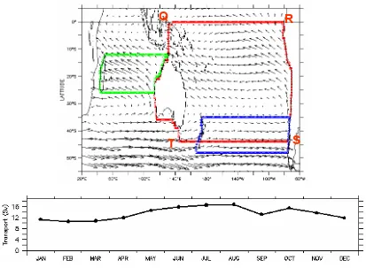
_{. (G2)}

Here, fQ and fT are the Coriolis coefficient at Q and T latitude, ρ0 is the mean water density. Both the streamfunction and the steric heights have been calculated for NCEP and ERA40 wind products, with the Indonesian Throughflow Passage open in a quasi-realistic topographic setting. The data provides monthly, annual mean and seasonal outputs of both variables in NetCDF format. This data is now available from the Tasmania Partnership of Advanced Computing (http://www.tpac.org.au). The Indonesian Throughflow, which is the path integral of the wind stress around the red loop QRST (upper panel, Fig. 2.1, based on that calculated using NCEP winds), shows a realistic seasonal cycle, strongest in southern winter and weaker in southern summer (lower panel, Fig. 2.1).

within which a trend is to be determined. These time scales have been calculated by previous studies for the South Pacific (e.g., Qiu and Chen, 2006, see Fig. 2.2). For example, at 45oS, it would take 22 years to complete the full Rossby wave adjustment process from the South Pacific's eastern boundary to its western boundary.

To determine the wind-driven South Pacific circulation trend at this latitude from 1978-2003 (e.g., Cai, 2006), which is 25 years, the Island Rule can be applied. At any latitudes north of 45oS, e.g., in the tropics, where the Rossby wave adjustment time scale is much shorter, the Island Rule is applicable. For the same time duration (1978-2003) discussed above, one can use the Island Rule to calculate maps of the wind-driven circulation trends. This is discussed in Chapter 5.

Figure 2.1: Upper panel, illustration of the Island Rule in the Indo-Pacific system, superimposing on annual mean winds. Three islands are included. For island such as Australasia, the circulation around the island can be obtained from the path integral of the wind stress around a path like the red loop QRST. Lower panel, transport in (absolute value) using NCEP monthly mean winds for Australasia, which is the modelled Indonesian Throughflow.

Q

T

S

R

Q

T

S

[image:32.595.95.508.288.591.2]

Figure 2.2: Time [years] required for the long baroclinic Rossby waves to traverse the South Pacific Ocean from the eastern boundary to the west (from Qiu and Chen, 2006). Notice that the contour intervals are not uniform.

Figure 2.3: Wind-driven climatological circulation for southern summer (upper panel) and southern winter (lower panel) based on NCEP winds. Unit in Sv (1 Sv = 106 m3 s-1).

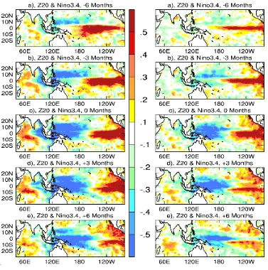
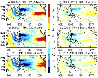
Another example is the decadal difference in the Pacific discharge/recharge via Sverdrup transport. The Pacific Ocean climate experienced a shift towards a warm state in the late 1970s, with marked changes in the ENSO properties and in many other circulation fields. During the post-1980 period, El Niño events are stronger than La Niña events contributing to significant difference in the mean circulation between the pre- and post-1980 periods. In the post-post-1980 periods, the equal Pacific circulation features weaker equatorial easterlies, stronger positive curls from the equator to 5oN and negative curl in the 5oS – 15oS (Fig. 2.4a). The curls, through Sverdrup balance promotes a greater discharge of heat from the equatorial region and hence a shallower equatorial Pacific thermocline in the post-1980 period (Fig. 2.4b) (Jin, 1997a; 1997b; Meinen and McPhaden, 2000), consistent with an El Niño-like multidecadal-long condition for the post-1980 period. On interannual time scales, the discharge signal is transmitted into the WA coast and radiates into the IO, leading to a shallower mean thermocline off the WA coast and throughout the southern tropical IO (Fig. 2.4b).

Wind-driven Eastern Australian Current Dec. Jan. Feb. average

Super-gyre circulation

Figure 2.4: Difference in 20-year averaged a) wind stress curl (N m-3) based on ERA40 winds, and b) thermocline depth (m) between the pre- and post-1980 period (post-1980 minus pre-1980) based on the Simple Ocean Data Assimilation (SODA) (Carton and Giese, 2007).

Figure 2.5: Decadal difference in wind-driven circulation (1981-2000 average minus the 1960-1980 average). Unit in Sv. The post-1980 period features stronger ENSO, with greater discharge of heat from the equatorial Pacific to the tropical latitudes.

Chapter 3: Indo-Pacific Teleconnection

In this Chapter, we address the process of the Indo-Pacific oceanic teleconnection through the Indonesian Throughflow passage. We then discuss the robustness of the teleconnection in terms of differences between the pre-1980 and post-1980 period. As already alluded in the Chapter 1, the motivation is to unravel the dynamics of rainfall variability over Australia, because previous studies have demonstrated a linkage between variability of EIO SSTs and South East Australia (SEA) rainfall, and a strong influence of Pacific variability and occurrence of the IOD since 1980.

The main findings reported in this Chapter are:

o The transmission of the Pacific ENSO signals to the IO involves an off-equatorial Pacific pathway;

o The transmission of El Niño discharge signals from the Pacific to the IO is far stronger during the post-1980 period, therefore contributing to the shallowing of the EIO thermocline and to the higher occurrence of stronger IOD events;

o This multidecadal difference is essential for explaining the structure of the temperature trends in the IO.

This chapter covers contents of published papers arsing from, and contributed to by this Ph. D project. The candidate initiates the original idea of, and leads the analysis of one paper (Shi et al., 2007), and contributes to the other two papers (Cai et al., 2007; Cai et al., 2005c).

3.1 Background

3.1.1 Teleconnection between EIO SST and SEA rainfall

While rainfall in north-eastern Australia (e.g. Queensland) is mainly affected by SST anomalies of the equatorial eastern Pacific Ocean region, there is no doubt that variability of the EIO SST has a great impact on the rainfall over Australia’s southeastern states (Smith, 1993; Smith et al, 2000; Ansell, 2000; Ashock et al.,