Relationship Between Velocity of Contraction and Force Applied On Air Muscles

Rochester Institute of Technology

RIT Scholar Works

Theses Thesis/Dissertation Collections

12-2016

Relationship Between Velocity of Contraction and

Force Applied On Air Muscles

Aniruddha Sudhir Phatak

asp2209@rit.edu

Follow this and additional works at:http://scholarworks.rit.edu/theses

This Thesis is brought to you for free and open access by the Thesis/Dissertation Collections at RIT Scholar Works. It has been accepted for inclusion in Theses by an authorized administrator of RIT Scholar Works. For more information, please contactritscholarworks@rit.edu.

Recommended Citation

Relationship Between Velocity of

Contraction and Force Applied

On Air Muscles

by

Aniruddha Sudhir Phatak

A Thesis Submitted in Partial Fulfillment of the Requirements for the degree of Master of Science in Mechanical Engineering.

Supervised by

Dr. Steven Day, Associate Professor Department of Mechanical Engineering

Kate Gleason College of Engineering Rochester Institute of Technology

Rochester, New York

December, 2016

Approved by:

_____________________________________________

Dr. Steven Day, Associate Professor

Thesis Advisor, Department of BioMedical Engineering

_____________________________________________

Dr. Kathleen Lamkin-Kennard, Associate Professor Committee Member, Department of Mechanical Engineering

_____________________________________________

Dr. Wayne Walter, Professor

Committee Member, Department of Mechanical Engineering

_____________________________________________

Dr. Agamemnon Crassidis, Professor

Thesis Release Permission Form

Rochester Institute of Technology Kate Gleason College of Engineering

Title:

Relationship Between Velocity of Contraction and Force Applied on Air Muscles

I, Aniruddha Phatak, hereby grant permission to the Wallace Memorial Library to reproduce my thesis in whole or part.

_____________________________________________ Aniruddha Sudhir Phatak

_____________________________________________

Acknowledgements

I would like to extend my sincere thanks to my advisor, Dr. Steven Day for his guidance, knowledge and continual support throughout my theoretical and experimental research which helped me to complete my thesis.

I would also like to thank my friend Shahan who helped me with the LabVIEW Programming. I would like to thank Drs. Wayne Walter and Kathleen Lamkin-Kennard for providing advice and material support, including air muscle supplies and instrumentation. I am also thankful to Mr. Jan Maneti, Mr. Rob Kraynik, and Carmen Azzaretti for helping me in the manufacturing of my test rig.

Abstract

Air muscles are simple pneumatic devices that have high potential to be used as robotic manipulators, as they have a behavior similar to biological motors or muscles. Hence, they have a wide range of potential applications in areas such as robotics, bio-robotics, biomechanics, and artificial limb replacements. In addition to the similarity to biological muscle, air muscles have the advantages of good power-to-weight ratio, being compliant, and low cost. This thesis primarily quantifies the relationship between velocity of contraction of air muscles and the force applied on it, which is a key characteristic of biological skeletal muscle. First, an experimental test rig was used to measure the velocity of contraction of air muscles as a function of applied force, supply pressure, and supply volumetric flow rate. Second, a theoretical model is proposed to quantify the relationship between the velocity of contraction and force applied on it and to explain the experimental results.

Three air muscles having different lengths and diameters were tested for loads ranging from 0 to 6 kg at 20 psi, 40 psi and 60 psi at two different flow rates. All three air muscles were made up of latex tubing sheathed with the Techflex, FlexoPet braided sleeve. The primary air muscle was 5 inches long, with the diameter of the inner tube measuring 3/4 of an inch. The second muscle had half the length (2.5 inches) and was the same diameter as the primary air muscle. The third air muscle was the same length as the first (5 inches long), but half of the diameter (3/8 of an inch). The velocity of the contraction was measured with the help of the linear potentiometer.

Contents:

Acknowledgements ... 3

Abstract ... 4

Nomenclature: ... 7

List of Figures: ... 9

1. Introduction ... 11

1.1 Problem Statement: ... 12

1.2 Objective: ... 12

2. Study of Air Muscles: ... 13

2.1. Nature of Air muscles ... 13

2.1.1. Compliant nature of Air muscles: [2] ... 13

2.1.2. Comparison of PAM’s and Skeletal Muscles: [2] ... 14

2.2. Classification of Air Muscles: [2] ... 14

2.2.1. Mckibben Braided Muscles: ... 14

2.2.2. Sleeve Bladder Muscle: [2] ... 25

2.2.3. Pleated PAM: [2] ... 25

2.2.4. Netted Muscles: [2] ... 26

2.2.5. Embedded Muscles ... 29

2.3. Existing Theoretical Model to Derive Equation of Force: [3] ... 30

2.4. Existing Experimental Model to Measure Contraction of Air Muscles at Varying loads: [4] ... 32

3. Experimental Model to Test Velocity of Contraction of Air Muscles at varying Forces: ... 36

3.1. Design and Building of the Experiment Test rig ... 36

3.2. Working of the Test Rig: ... 37

3.2.1. Data Acquisition ... 38

3.2.2. Analysis of Readings: ... 40

3.2.3. Example of Analysis of raw Data ... 40

3.3. Results: ... 42

Specifications of the air muscles used for the experiment are as follows: ... 42

4. Theoretical Model to Quantify Relationship Between Velocity of Contraction and Force Applied on it. 53 4.1. Procedure: ... 53

4.2. Results: ... 56

5. Discussion: ... 63

7. References: ... 70

8. Appendix: ... 72

8.1. Instruction Set to operate Experimental Test Rig. ... 72

8.2. Raw Data Plots of Experimental Model: ... 73

8.3. Experimental Raw Data: ... 74

8.4. Theoretical Model Data Sheet ... 77

Nomenclature:

PAM = Pneumatic Artificial Muscle

PPAM = Pleated Pneumatic Artificial Muscle P = absolute gas pressure

P0= atmospheric pressure

F = force

P’ = relative internal gauge pressure si= total inner surface

dsi = the area vector

dli = inner surface displacement

dV = volume change.

D = diameter of Air Muscle at particular position D0 = diameter of the air muscle at normal position

b = braided length of the air muscle

𝜃 = braided angle at a specific position L = contracted length of Air Muscle L0 = normal length of Air Muscle

Ls= stretched length of Air Muscle

tk= thickness of the air muscle (shell and bladder) n = number of turns of the thread

C = Circumference Nc = number of nodes

G = distance between two nodes Ds = diameter of one strand

WB = width of each strand

N = number of strands

𝑁_𝑐 = number of nodes in one circulation of the circumference S = number of parallel strands

Lmin = minimum length of muscle at maximum contraction

c = compliance k = stiffness

Rmin = minimum radius of air muscle 𝜀 = strain

𝑎= dimensionless factor for elasticity

Ffriction = resisting force caused due to Dry friction is air muscle

Scontact = total contact area between the strands of whole muscle

Nconatcts = total number of crossover points

Sone = area of one contact polygon

fs= coefficient of friction

V= volume of air inside the air muscle M=mass of air inside the air muscle

List of Figures:

Figure 1: Construction details of Air Muscle [4] ... 15

Figure 2: Length of Air Muscle (a): Stretched Air Muscle (of maximum length Lm). [4] ... 16

Figure 3: Geometry of Air Muscle- Polyester braid angle (a). Geometry of actuator. Middle portion of the actuator is modeled as perfect cylinder with length L, diameter D. 0, angle between braded thread and cylinder long axis, n, number of turns of thread, and b, thread length. (b) Relationship between above parameters is illustrated by triangle. [3] ... 16

Figure 4: McKibben Muscle tension (N) and hysteresis at isobaric conditions (0, 100, 200, 300, 400 and 500 kPa), (a) Nylon braid, (b) fiberglass braid. [3] ... 17

Figure 5: Braid material (a) and unrolled (b) [6] ... 18

Figure 6: Braid structure assuming single strands. [6] ... 19

Figure 7: One single braid crossover point. [6] ... 22

Figure 8: Orthotropic material layers (a), Meshed model of a PAM (b) [5]... 23

Figure 9: Linear-static FEA results [5] ... 24

Figure 10: Pleated Muscle, fully stretched and inflated. [2] ... 25

Figure 11: Yarlott Muscle. [2] ... 26

Figure 12: ROMAC, standard version (a) and miniature version (b) [2] ... 28

Figure 13: Kukolj Muscle. [2] ... 28

Figure 14: Morin Muscle Designs [2] ... 30

Figure 15: Comparison of Contraction of Air Muscles vs. Pressure Plots [4] ... 33

Figure 16: Comparison of Volume Trapped vs. Pressure Plots [4] ... 33

Figure 17: Behavior of Air Muscle at constant pressure. [4] ... 34

Figure 18: Operation of Air Muscle at constant load. [4] ... 35

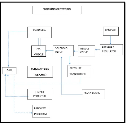
Figure 19: Block Diagram of Working of Test Rig. ... 36

Figure 20: Experimental Test Rig ... 38

Figure 21: Displacement vs. time plot of experimental data. ... 41

Figure 22: Velocity of contraction vs. time plot at 10 N, V1 ... 42

Figure 23: Comparison of maximum velocities of A1, A2 and A3 at 20 psi at 0N and 10 N load conditions, measured at both the volume flow rates (R1 and R2). ... 44

Figure 24: Comparison of maximum and average velocities of A1, A2, A3 at 20 psi at R1, R2. ... 44

Figure 25: Comparison of maximum velocities of A1, A2 and A3 at 40 psi at 0N and 10 N load conditions, measured at both the volume flow rates (R1 and R2). ... 46

Figure 26: Comparison of maximum and average velocities of A1, A2, and A3 at 40 psi at R1, R2 ... 47

Figure 27: Comparison of maximum velocities of A1 and A2 at 60 psi at 0N and 10 N load conditions measured at both the volume flow rates (R1 and R2). ... 48

Figure 28: Comparison of maximum and average velocities of A1 and A2 at 60 psi at R1, R2. ... 50

Figure 29: Comparison of maximum change in lengths (Delta L) at 20, 40, and 60 psi for air muscle A1. 51 Figure 30: Comparison of Delta L at 20, 40, and 60 psi for air muscle A2. ... 51

Figure 31: Comparison of Delta L at 20 and 40 psi for air muscle A3. ... 52

Figure 32: Static Model ... 54

Figure 33: Dynamic Model ... 55

1.

Introduction

An air muscle is a simple pneumatic device which was developed by J. L. Mckibben in the 1950s. It was primarily developed for polio patients as an orthotic appliance according to Baldwin [4, 7]. Initially, these muscles were made up of pure latex rubber. As they closely resemble the natural muscle when actuated by air, they became known as air muscles. In the late 1980s, the Bridgestone Rubber Company commercialized these rubber actuators, and since then, many types of air muscles have been used as manipulators mainly for prostheses and orthotics [4, 8]. A Mckibben Air muscle consists of a rubber bladder surrounded by a braided mesh shell which is attached to an air fitting on one end and two mechanical fittings at both ends. As the internal bladder is pressurized, it expands and pushes against the mesh to increase its volume. Due to high non-extensibility of the threads in the braided mesh shell, when activated, the air muscle’s diameter increases and produces tension if coupled with a mechanical load, producing a contractive force.

One of the potential uses of air muscles include manufacturing of dexterous robotic hand having good control of all the fingers in order to fulfill basic hand operations like catching, picking, pulling, and placing objects. Another important application is to make an artificial leg that can walk, run, and jump like a human. Researchers Hannaford et al. built an Anthropomorphic Biorobotic Arm which consisted of fifteen Mckibben muscles [2, 9]. The main purpose was “to improve the understanding of the reflexive control of human

movement and posture." Grodski and Immega [2, 10] used ROMACs to control a tele operated arm having one degree of freedom (dof) with the help of myoelectric signals generated from the human operator’s triceps and biceps. Specific position and control over stiffness of the

1.1

Problem Statement:

Air Muscles are currently finding a place in a wide range of applications like robotics, bio-robotics, biomechanics, and artificial limb replacement. As the characteristics of air muscles resemble the skeletal muscles they can be used to perform high end hand applications like assembling of very minute components etc., once coupled with neural network systems and precise sensors. To achieve accurate positioning and gripping force in all these applications it is necessary to understand the relation between force exerted by the air muscle and its velocity of contraction.

I did not find any literature regarding velocity of contraction during my course of research. My research question primarily asks, what is the exact relationship between the force acting on the air muscle and the corresponding velocity of its contraction for varying air pressures and volume flow rates? Given this relationship, future designers can achieve specific force-velocity relationships, which will help development of biometic actuators. For example, we can achieve desired movement of the fingers or the legs to perform the required operations by knowing the mathematical equation force and velocity.

1.2

Objective:

1. To build a test rig which to measure the velocity of contraction of air muscles when different forces are applied by taking into account the effect of varying pressures and volume flow rates.

2.

Study of Air Muscles:

2.1.

Nature of Air muscles

Pneumatic actuators are extensively used in automation industries. Lately pneumatics are widely used in robotics as the main source of power for achieving necessary motion. Compliant nature of pneumatics is of prime importance as robotics often deal with interaction between man and machine or between robots and delicate objects which are to be handled by robots. The compliant nature due to the compressibility of air and the control over operating pressure makes soft and safe interaction between pneumatically handled robots and the corresponding objects possible. Conventionally, hydraulic and electric drives were used in robotics. Unlike skeletal muscle, these systems often are fixed displacement systems that will move to a certain position regardless of the applied force. In order to obtain an actuator system with behavior that reacts to this load, these systems typically need complex feedback loop systems to attain the required compliant nature. Pneumatic Artificial Muscles (PAMs) can be considered as contractile and linear motion engines which are operated by air pressure. [2]

2.1.1.

Compliant

: [2]

Pneumatic actuators show compliant nature because of compressibility of the gas. Change in force is directly proportional to change in length when pressure is maintained constant, so the PAM behaves like a spring. Compliance, c is given as-

𝑐−1 _{= 𝐾 =} 𝑑𝐹 𝑑𝐿 = −

𝑑𝑝′ 𝑑𝑉 (

𝑑𝑉 𝑑𝐿)

2

− 𝑃′𝑑2𝑉

𝑑𝐿2 (1)

Here, K represents stiffness.

Assuming the polytropic process (𝑃′ ∗ 𝑉𝑛′ _{= 𝑧) inside of the muscle, equation can be written}

as-

𝑐−1_{= −𝑛′} 𝑃′+𝑃0

𝑉 ( 𝑑𝑉 𝑑𝐿)

2

− 𝑃′𝑑2𝑉

𝑑𝐿2 (2)

As both terms depend upon pressure, compliance (equivalent to the spring constant) can be adapted by controlling the pressure. [2]

2.1.2.

Comparison of PAM’s and Skeletal Muscles: [2]

PAM’s resemble skeletal muscle in such a way that both are linear contractile actuators that show a decreasing load-contraction relation Fluidic actuators i.e. PAM’s generate motion

only in one direction. Just like skeletal muscles two actuators are needed to be coupled so that bidirectional motion can be achieved one actuator for each direction. One muscle moves the load while the other acts as brake to stop the load at desired position. To change the direction of moving load the functions of the muscles are interchanged. The antagonistic coupling can be used for linear as well as rotational motion. It can also control the joint compliance as in the skeletal muscles.

The following are the differences between the biological muscles and PAM’s:

 Skeletal muscles do not change volume during contraction.

 Unlike PAM’s, they have a modular structure having large number of parallel and series connections of microscopic contractile systems.

 Human muscles have internal force and strain gauges.

2.2.

Classification of Air Muscles: [2]

2.2.1.

Mckibben Braided Muscles:

In my research, I have studied a specific type of air muscle, the Mckibben Air Muscle, which is the most widely used type of air muscle.

2.2.1.1.

Construction of Mckibben Air muscle:

rubber bladder is filled by the air it seeks to expand. The nylon mesh resists the rubber tube to expand along the diameter. The inherent characteristic of the nylon mesh is such that the maximum diameter of the nylon mesh increases with decrease in its length. The unique nature of the woven nylon allows the expansion of air muscle in terms of diameter tube until a certain limit. After this stage as the pressure increases the air muscle gets contracted thus decreasing its length and subsequently increasing its diameter and in turn giving more space for the expansion of the inner tube. Hence as the pressure increases net result would be such that the length of the air muscle decreases while it expands in term of the diameter. If a load is attached to the sealed end it will be displaced to the amount of the decreased length provided the load is in the operating range. This pulling action on the load when effectively utilized could provide the necessary motion. [4]

As the Mckibben muscle is pressurized by air, the rubber tube is pressed against the mesh laterally. Thus, internal pressure is balanced by the tension in the fiber of the mesh due to the curvature of the rubber tube. When the external force is applied on the air muscle it gets balanced by this axial tension which is integrated at the end points of the mesh. If the input pressure of the air is less than the threshold pressure the rubber tube gets inflated, however

doesn’t come in contact with outer mesh. Hence sufficient tension is not produced in the mesh, which in turn prevents the air muscle to bulge and thereby restricts the contractive movement to uplift the external force. [2]

There are 3 positions of air muscle respectively- Normal, stretched and actuated length.

Figure 2: Length of Air Muscle (a): Stretched Air Muscle (of maximum length Lm). [4]

(b): Air Muscle (of length L0) in normal state.

(c): Air Muscle (of length L ) under pressure.

a. b.

Figure 3: Geometry of Air Muscle- Polyester braid angle (a). Geometry of actuator. Middle portion of

the actuator is modeled as perfect cylinder with length L, diameter D. 0, angle between braded thread

and cylinder long axis, n, number of turns of thread, and b, thread length. (b) Relationship between

The typical static behavior of an air muscle can be demonstrated by an example muscle from Tondu et al. This is described here only for the purpose of showing characteristic behavior of a muscle. Following are the values mentioned by Tondu et al. [2, 11] 650 N at rest length, 300 N at 15% contraction, 0 N a 30% contraction at pressure equal to 300 kPa. Rest length equal to 150 mm, diameter = 14 mm, and weight = 50 g.

The higher the maximum pressure which muscle can withstand, the higher is the energy which can be transferred. However, as the toughness of the diaphragm i.e. the inner bladder is increased to increase the maximum pressure, its threshold pressure also increases. Chou and Hannaford [3] have reported values of hysteresis width ranging from 0.2 cm – 0.5 cm and height varying from 5 to 10 N for a nylon braid muscle of 14 cm rest length and 1.1 cm rest diameter. The threshold pressure reported was 90 kPa.

Figure 4: McKibben Muscle tension (N) and hysteresis at isobaric conditions (0, 100, 200, 300, 400

and 500 kPa), (a) Nylon braid, (b) fiberglass braid. [3]

2.2.1.2.

Braid Structure: [6]

The braid structure plays very important role in deciding performance characteristics and preventing over inflation. The expansion of the muscle is radial and its resulting contraction is done due the virtue of braid structure. Even the settling limit of contraction and dilation depends upon the braid structure.

The contraction of the pneumatic muscle is mostly around 30-35% (Caldwell, Medrano-Cerda and Goodwin 1995) and is given in terms of braid angle. The maximum contraction of the muscle is achieved at the inter braid angle equal to 54 degrees. The maximum diameter of the muscle or the minimum braid angle are limited by due to maximum force between adjacent strands of the braid or due to larger size of the bladder which prevents full expansion of the outer bladder. If the bladder diameter is small enough then the braid angle will depend upon weave pattern (typically a 2/2 Twill (Braidweaver 2005), material of the fiber and its diameter. The range of contraction of the muscle varies from maximum to minimum braid angle. Hence by lowering the braid angle dynamic range of the contraction can be increased.

Figure 5: Braid material (a) and unrolled (b) [6]

Theoretical calculation for minimum braid angle-

between two nodes. C is the circumference of the air muscle and 𝑁_𝑐 is number of nodes in one circulation of the circumference. Figure (b) shows 𝑁_𝑐=3. As per (Schulte 1962)

𝐷₀ = 𝑏

𝑛𝜋 (3)

Therefore

𝑙 =𝜋.𝐷0

2.𝑁𝑐 (4)

The node separation is given by

𝐺 = 2𝑙 sin Ɵ (5)

The structure of the braid shown in Figure assumes that there is only one strand in each path having thickness𝑊𝑏. In reality number of parallel strands follow in each path, but principle

of the analysis remains the same.

𝑋 = 𝑌 cos Ɵ ⇒ Y = Wb

2∗cos Ɵ (6)

Figure 6: Braid structure assuming single strands. [6]

Ɵ_𝑚𝑖𝑛 =sin

−1₍2.𝑊𝑏.𝑁𝑐 𝜋𝐷0 )

2 (7)

By substituting thickness in terms of diameter of one strand (𝐷𝑠) and number of parallel

strands (S)

𝑊_𝑏 = 𝐷_𝑠. 𝑆 (8)

Also

𝑁_𝑐 = 𝑁

2.𝑆 (9)

Where N is number of strands to create complete muscles. Therefore, the minimum braid angle is given by

Ɵ_𝑚𝑖𝑛 =sin

−1₍𝐷𝑠.𝑁 𝜋𝐷0)

2 (10)

This calculated angle remains constant irrespective of its length if Ds, S, and N are assumed to remain constant. Maximum dilated length can be calculated by using the equation by Schulte (1962). 𝐿𝑚𝑎𝑥 is of more importance for practically design as robotic application.

Therefore

2.2.1.3.

Friction/Hysteresis: [6]

𝐿𝑚𝑎𝑥 = 𝑏 cos Ɵ𝑚𝑖𝑛= 𝐿𝑚𝑎𝑥 = 𝑏 cos (

sin−1(2.𝑊𝑏.𝑁𝑐

𝜋𝐷0 )

2 ) (11)

the contraction of the muscle while subtracting it during extension. Although Tondu and Lopez further tried to quantify the offset value by modeling the friction as it was a static based model, it could not provide accurate force data (Schulte 1962; Chou and Hannaford 1996; Tsagarakis and Caldwell 2000; Davis et al. 2003). As per Tondu and Lopez (2000) a

parameter K which “tunes the slope of the considered static model” is introduced to

overcome the issue. Although the model is more accurate than Chou and Hannaford, it relies greatly on the experimental data.

2.2.1.4.

Braid Contact Area: [6]

The braid strands rub against each other and hence friction is produced which should be included in the mathematical model. The expression for static dry friction of the braid as per Tondu and Lopez (2000) is given by-

𝐹_{𝑓𝑟𝑖𝑐𝑡𝑖𝑜𝑛} = 𝑓_𝑠∗ 𝑆_{𝑐𝑜𝑛𝑡𝑎𝑐𝑡}∗ 𝑃 (12) Where 𝐹_{𝑓𝑟𝑖𝑐𝑡𝑖𝑜𝑛} denotes resisting force caused by the friction, fs is the coefficient of friction (0.15 – 0.25 for a nylon and 𝑆_{𝑐𝑜𝑛𝑡𝑎𝑐𝑡} is the contact area between the strands. Due to the weaving of the strands, contact varies according to the braid angle. Hence contact area should be calculated. One braid crossover point is taken into account to

calculate

𝑡𝑎𝑛𝜃 = 𝑥

𝑦 (13)

sin 𝜃 = 𝑊𝐵

2𝑦 (14)

𝑆𝑜𝑛𝑒 = 2 ∗ 𝑥 ∗ 𝑦 (15)

𝑆𝑜𝑛𝑒 =

𝑊𝐵2

2 sin 𝜃 cos 𝜃 (16)

𝑊_𝐵 is the width of the braid strand. It is assumed that a single strand fallows each path. As in the practical case number of parallel strands are used where 𝑊𝐵 is the total width of the

strands. Therefore, the total contact is given by

𝑆𝑐𝑜𝑛𝑡𝑎𝑐𝑡𝑠 =

𝑁𝑐𝑜𝑛𝑡𝑎𝑡𝑐𝑠𝑊𝐵2

2 sin 𝜃 cos 𝜃 (17)

N contacts denote total number of crossover points in the air muscle.

Figure 7: One single braid crossover point. [6]

When the air muscle is at maximum dilation, the braid is minimum and hence it can be assumed that the whole area of the muscle is made up of crossover points instead of experimentally calculating them.

By using length, diameter and minimum θ equations surface area can be calculated as fllows-

𝑆𝑢𝑟𝑓𝑎𝑐𝑒 𝐴𝑟𝑒𝑎 = 𝜋 ∗ 𝐷𝑚𝑖𝑛∗∗ 𝐿𝑚𝑖𝑛= 𝑆𝑜𝑛𝑒∗ 𝑁𝑐𝑜𝑛𝑡𝑎𝑐𝑡𝑠 (18)

By substituting above equations:

𝑁_{𝑐𝑜𝑛𝑡𝑎𝑐𝑡𝑠} =2∗𝑏2∗sin2𝜃𝑚𝑖𝑛∗ cos2𝜃𝑚𝑖𝑛

Therefore,

𝑆𝑐𝑜𝑛𝑡𝑎𝑐𝑡𝑠 = 𝑆𝑜𝑛𝑒∗ 𝑁𝑐𝑜𝑛𝑡𝑎𝑐𝑡𝑠 (20),

Therefore,

𝑆_{𝑐𝑜𝑛𝑡𝑎𝑐𝑡𝑠} =𝑏2∗sin2𝜃𝑚𝑖𝑛∗ cos2𝜃𝑚𝑖𝑛

𝑛∗𝑠𝑖𝑛𝜃∗𝑐𝑜𝑠𝜃 (21)

As a result, the frictional force can be calculated by substituting 𝑆_{𝑐𝑜𝑛𝑡𝑎𝑐𝑡𝑠} in equation 12.

2.2.1.5.

Finite Element Modeling: [5]

The FE modeling was primarily undertaken to verify force generated due to applied load at certain pressures. Linear-static solver in educational FEA code LUSAS was used for the modeling. The PAM was considered as cylinder having orthotropic material which represent is membrane and braids accordingly.

(a) (b)

Figure 8: Orthotropic material layers (a), Meshed model of a PAM (b) [5]

loads are increased to apply force on the PAM at the free end. By applying FE shell mesh to the structure loads and displacement is achieved in every direction along the Cartesian axis system. Relation of force with displacement was observed for certain pressures. Also, stiffness of PAM actuated with constant pressure was plotted against load applied on the PAM. Load is increased from 10 N to 100 N while the pressure is varied from 100 KPa to 500 KPa. The FE model can be modified by including nonlinear material model so that hyper elastic membrane stretching–expansion can be incorporated.

Figure 9: Linear-static FEA results [5]

(a)Fully inflated at 500 kPa (L=263.55 cm)

(b) Axial load 30 N (L = 273.83 mm)

(c) Axial load 70 N (L = 287.53 mm)

2.2.2.

Sleeve Bladder Muscle: [2]

These are different type of braided air muscles. The difference between sleeve bladder muscles is that the inner bladder is not connected to the mesh at the two ends with the help of the clamps as in the case of McKibben muscles. Here, only braid is connected to the end fitting. The advantage of these kinds of PAM’s are that they are very easy to construct. A

sleeved Bladder Muscle is a subject of the patent of Bullens.

2.2.3.

Pleated PAM: [2]

Pleated PAM (PPAM) was developed by Daerden recently. It consists of rearranging kind of membrane having no mesh. Hence it implies that there is no material strain during the inflation of the muscle. The membrane has number of pleats along the axial direction which unfold during its expansion. The stresses in membrane are in parallel direction and are kept negligibly small.

Figure 10: Pleated Muscle, fully stretched and inflated. [2]

These stresses decrease with the increase in number of pleats and hence very less energy is required to expand the membrane as compared to the other air muscles. Also, hysteresis which is a major drawback of braided muscles, is not seen in PPAM as the friction between membrane and mesh is totally absent. Very low amount of energy is lost during the bulging

of the flexion of the muscle. The characteristics of the PPAM’s depend upon ratio of full length

to minimum diameter, strain behavior of material of the membrane, rate of contraction and the applied pressure. Contraction force can be represented with following formula:

𝐹𝑡 = 𝜌𝐿02𝑓𝑡(𝜀, 𝐿0

𝐿₀, represents the muscles full length, 𝑅 is the minimum radius, a is the dimensionless factor accounting for the elasticity of the membrane. ft is dimensionless function which depends

upon rate of contraction, geometry, and behavior of material. The factor of elasticity can be eliminated by using material having high tensile strength and stiffness.

The PPAM is very strong in comparison to other PAM’s having greater linear displacement

without having any hysteresis. When weight and compliance are of prime importance, use of

PPAM’s is ideal. Example of PPAM’s in robotics are jumping, walking or running robots, grippers which can provide grip with varying firmness and flexible robot arms. As compared to braided muscles accurate positioning and controlling can be achieved easily and hence these are more suitable to fulfill above objectives.

2.2.4.

Netted Muscles: [2]

The main difference between braided and netted muscles is that density of the mesh in netted muscle is higher as the mesh has large number of holes. Hence the stretching membrane in the netted mesh can withstand relatively lower pressures. So these kind of muscles usually have pleated i.e. rearranging internal bladder.

2.2.4.1.

Yarlott Muscle

This is a US patented muscle developed by Yarlott. The bladder is made up of an elastomer having prolate spheroidal shape. The bladder is netted by series of strands running axially, end to end to avoid the elastic expansion of membrane. Instead of net, a single strand can be wounded helically about the shell.

When the muscle is fully inflated, it looks like a spheroid. As the air is removed from the muscle the axial strands straighten to force the bladder in its shape characterized by series of ridges and valleys. The surface area of bladder does not change as the rearranging surface accounts for the expansion of the muscle. Since the stretching of the bladder is reduced in this way, more pneumatic energy is transformed into mechanical power. Though the axial strands would be fully straightened and under tremendous tension during the complete elongation, it is not yielded due to its material properties. Yarlott muscles mostly operate at low gauge pressures.

2.2.4.2.

ROMAC

(b)

Figure 12: ROMAC, standard version (a) and miniature version (b) [2]

2.2.4.3.

Kukoji Muscles

It is a variation of Mckibben muscle having open-meshed net unlike tightly woven braid. There is a gap between the membrane and the mesh during the no load condition. It disappears as the muscle is applied with high extending load. The condition of the muscle when not activated with pressure however applied with the load such that net fits the diaphragm is the fully extended condition. In these muscles as the net contracts at a higher rate than membrane, to avoid the buckling at the ends initial gap is provided.

The figure shows the muscle in different cases like uninflated, fully elongated and actuated to pick up the load respectively.

2.2.5.

Embedded Muscles

The following are different kinds of embedded muscles:

2.2.5.1.

Morin Muscle

Figure 14: Morin Muscle Designs [2]

2.2.5.2.

It basically follows the design of Morin muscles. The elastomeric membrane is embedded by glass filaments along the vertical axis. The so formed membrane has very high modulus of elasticity along the direction filaments as compared to direction perpendicular to it. As discussed earlier as there is no friction with outer mesh, the muscle has very less hysteresis. Also, the threshold pressure is very low. As radial expansion is high the pressure is limited to 100 kPa. As per Baldwin 1600 N force can be lifted by the muscle. Life tests indicate operating life of 10000 to 30000 cycles when a weight of 45 kg was alternatingly lifted and lowered at about 100 kPa.

2.3.

Existing Theoretical Model to Derive Equation of Force: [3]

The Static Physical model of Mckibben Muscles derived by Chou and Hannaford which give us the formula for force applied on the air muscles is studied in this section. [3]

Work input done on the Mckibben Muscle as the pressurized air inflates the air muscle is given by

𝑑𝑊𝑖𝑛 = ∫ (𝑃 − 𝑃_𝑆 0)𝑑𝑙𝑖. 𝑑𝑆𝑖

𝑖 = (𝑃 − 𝑃0) ∫ 𝑑𝑙𝑖. 𝑑𝑆𝑖 = 𝑃

′_𝑑𝑉

𝑠𝑖 (23)

The output work is associated with volume change as the actuator shortens is given by

𝑑𝑊𝑜𝑢𝑡 = −𝐹𝑑𝑙 (24)

As per the law of conservation

𝑑𝑊_𝑜𝑢𝑡 = 𝑑𝑊_𝑖𝑛 (25)

−𝐹𝑑𝑙 = 𝑃′𝑑𝑉 (27)

𝐹 = −𝑃𝑑𝑉

𝑑𝐿 (28)

Assumptions:

The extensibility of shell threads is very low; volume of the air muscle depends on its length. The middle portion of the air muscle is assumed to be a perfect cylinder having L and D as the length and diameter of the cylinder.

𝐿 = 𝑏 𝑐𝑜𝑠𝜃 (29)

𝐷 = 𝑏 sin 𝜃

𝑛𝜋 (30)

Therefore, the volume is

𝑉 =1

4𝜋𝐷

2_{𝐿 (31)}

𝑉 = 𝑏3

4𝜋𝑛2𝑠𝑖𝑛

2_{𝜃𝑐𝑜𝑠𝜃 (32)}

𝐹 = −𝑃′𝑑𝑉 𝑑𝜃⁄

𝑑𝐿 𝑑𝜃⁄ (33)

Therefore

𝐹 =𝜋𝐷02𝑃′

4 (3𝑐𝑜𝑠

2_{𝜃 − 1) (34)}

𝐷₀ = 𝑏/𝜋𝑛is the diameter when θ is equal to 90 degrees.

Effect of thickness of the nylon shell and the bladder on the length of the air muscle [3]: When the thickness (tk) of the shell and the bladder is considered, the volume can be

expressed as follows:

𝑉 =1

4𝜋(𝐷 − 2𝑡𝑘)

2_{𝐿 (35)}

Therefore, the formula for the force developed by the air muscle can be given by

𝐹 =𝜋𝐷02𝑃′

4 (3𝑐𝑜𝑠

2_{𝜃 − 1) + 𝜋𝑃}′_[𝐷

0 ∗ 𝑡𝑘(2 ∗ 𝑠𝑖𝑛𝜃 − 1

𝑠𝑖𝑛𝜃) − 𝑡𝑘

2_{] (36)}

This equation gives more accurate results as compared to equation (34). However, thickness, tk, is often neglected in order to find the change in length.

2.4.

Existing Experimental Model to Measure Contraction of Air

Muscles at Varying loads: [4]

"Theoretical and Experimental Modeling of Air Muscle" [4] paper is discussed in this section. It describes testing of air muscles to measure the contraction of the air muscles at different loads. Effect of varying pressures was also taken into account during the experiment. The relationship between volume and variation of pressures at different loads is also analyzed. The experimental setup included a compressed air supply, air muscles, a pressure regulator, 0.5 kg weights, and a travelling microscope to measure the length contraction. Pressurized air was induced in the air muscle, and the contraction of the air muscle was observed for the respective loads.

The pressure increase from 30 psi to 80 psi is similar to te pressure increase mentioned in the paper, as well.

a. b.

Figure 15: Comparison of Contraction of Air Muscles vs. Pressure Plots [4]

For the second test, volume trapped in the muscle was plotted against varying pressures at different loads. It was observed as the pressure increases in steps, the volume increases and the contracted length decreases for a constant load.

Figure 16: Comparison of Volume Trapped vs. Pressure Plots [4]

Similarly, I have also plotted the graph of volume trapped vs. pressure, and again the trending curves are similar to those in the published plot. Volume displaced during contraction was in the range of 0–5 ml as compared to the 0–11 ml range in the published plot. Once again pressure was increased from 30 to 80 psi. The only difference between these two plots is that my theoretically modeled plot shows the least volume displaced for the highest load, while the published plot has the highest volume displaced for the highest load. As the load applied to the air muscle increases, the contraction will be less, as the load acts against the direction of contraction. The figures in this paper demonstrate that as the

0 10 20 30

30 50 70 90

C o nt rac ti o n o f A ir M us cl es,m m Pressure,psi

Pressure Vs Contraction of Airmuscle

1kg Load 3kg Load 5kg Load

0 1 2 3 4 5

30 40 50 60 70 80

Vo lum e, m l Pressure,psi

Volume Trapped in Air Muscle

load (i.e., applied force) is increased, the corresponding volume decreases. The error in the paper can be because of the experimental error while performing the same.

Following are the observations of the experiments mentioned in the published paper. For Pressure, P = constant

F1 > F2 > F3 v1 < v2 < v3 x1 > x2 > x3

Figure 17: Behavior of Air Muscle at constant pressure. [4]

Figure 18: Operation of Air Muscle at constant load. [4]

Also, if the pressure is kept constant and the load increases in steps, the contraction in length and the volume decrease.

The paper also discusses a formula for the length of an inflated air muscle in the following form:

𝐿 = √(𝑏2−(4∗𝐹∗𝜋∗𝑛2)/𝑃)

3 (37)

As per the formula above, the length of the air muscle will increase as the pressure increases. However, as per the basic characteristic of the air muscle, the length of the air muscle should decrease as pressurized air is induced in the air muscle. The reason for this discrepancy is that Ranjan et al. has incorrectly considered output work equal to positive product of force (F) and change in length (dl) while deriving the equation for force applied on the air muscle. However, the output work is associated with volume change as the actuator shortens and hence is given by:

𝑑𝑊_𝑜𝑢𝑡 = −𝐹𝑑𝑙 (24) Also, the input work is given by (23)

𝑑𝑊𝑖𝑛 = ∫(𝑃 − 𝑃0)𝑑𝑙𝑖. 𝑑𝑆𝑖 𝑆𝑖

= (𝑃 − 𝑃0) ∫ 𝑑𝑙𝑖. 𝑑𝑆𝑖 = 𝑃′𝑑𝑉 𝑠𝑖

And hence, the force developed in the equation should be negative times the product of pressure and change in volume. (28)

𝐹 = −(𝑃 ∗𝑑𝑉

𝑑𝐿)

Therefore, the error is incorporated in the final equation of length. Hence, the correct formula should be,

𝐿 = √(𝑏2+(4∗𝐹∗𝜋∗𝑛2)/𝑃)

3.

Experimental Model to Test Velocity of

Contraction of Air Muscles at varying Forces:

3.1.

Design and Building of the Experiment Test rig

Figure 19: Block Diagram of Working of Test Rig.

a T-shaped valve, which was fixed to the load cell. The load cell in turn was attached to the C-shaped bracket, which was fixed to the front plate. The front plate was connected to the 30 cm-long lead screw arrangement from the back side. This arrangement helped to adjust the position of the air muscle along the longitudinal axis. This adjustment was important to accommodate weights at the bottom of the air muscle and to position the linear potentiometer below the air muscle along the longitudinal axis. A course adjustment was provided so that the lead screw could be moved along the vertical axis in order to accommodate air muscles of various sizes, including bigger air muscles having varied lengths. The whole assembly rested on a base plate. A hook was attached to the base plate to hold the linear potentiometer in a straight position.

3.2.

Working of the Test Rig:

Figure 20: Experimental Test Rig

3.2.1.

Data Acquisition

The two sensors—namely the pressure transducer and linear potentiometer—are connected to SCB - 68 NI DAQ board. The DAQ in turn was connected to the computer with the help of a data cord so that it can communicate with LabVIEW 2012, which was installed on the computer. The LabVIEW program displayed following two graphs on the front panel:

3.2.1.1.

Pressure vs. Time Plot

LabVIEW program. Pressure was calibrated in psi, and time was represented in time. The linear equation used for the calibration of the pressure voltage into grams was (Y= 14.4 * X – 16.8). The equation was substituted in the block diagram of the program. The equation was found by increasing pressures incrementally from 30 to 80 psi with the help of the regulator, and the raw corresponding voltages were noted with help of the pressure transducer. The graph of voltage vs. real pressure was plotted, and the trade line equation was used for calibration. Real time pressure as well as raw pressure voltage were displayed on the panel.

Specifications:

Min voltage = +5volts Max voltage = -5volts

The signal from the pressure transducer was amplified and conditioned, and then the output was connected to AI channel 1 of DAQ board.

3.2.1.2.

Displacement vs time Plot

The displacement voltage was measured with the help of linear potentiometer and the data was processed such that displacement voltage vs. time graph was displayed on the panel. Also, real time voltage was displayed in a window.

Displacement voltage was directly converted into real displacement during the actual calculations by using the similar calibration technique like pressure. Displacement was then converted into velocity by using the slope of the displacement vs. time graph.

Specifications:

Min voltage = +5volts Max voltage = -5volts

The signal from the linear potentiometer was connected to AI channel 5 of DAQ board. Also, the time, given in seconds, was displayed on the front panel along with the count of the number of readings taken during one test.

Specifications:

Acquisition Mode: Continuous samples Samples to Read: 100

Rate: 1000Hz

The 12V solenoid valve, which was used to actuate the air muscle, was operated by a Measurement computing relay board. The relay board was operated with the help of the LabVIEW program. A special inbuilt program was used to communicate between the relay board and the LabVIEW program. With the help of this program, seven relays could be turned on by pressing the corresponding seven buttons on the front panel. One of the buttons was used to operate the solenoid valve.

3.2.2.

Analysis of Readings:

With the help of linear potentiometer readings saved in the Excel file, actual position displacement is measured by considering the voltage scale of the potentiometer. As the displacement is plotted against time, actual velocity is measured by finding the slope of the graph. From the velocity readings, maximum velocity and average velocity are measured for one of the contraction cycles observed by the air muscle. This process is carried out for the different sets of loads, pressures, and volume flow rates (restrictions) mentioned above. Sets of each type of velocity are plotted against forces ranging from 0–60N at three different pressures, namely 20 psi, 40 psi and 60 psi.

3.2.3.

Example of Analysis of raw Data

Figure 21: Displacement vs. time plot of experimental data.

In the figure 22., velocity of the contraction of air muscle is plotted against the time. With the help of displacement measurements at each time, velocity was measured. As demonstrated by the graph, velocity increases initially until a certain time and then it decreases gradually. The maximum velocity in this case is 2.251 in/s, which is measured by finding the maximum value amongst all the velocities in the time span of this contraction cycle. Similarly, the average velocity is found by measuring the average of the velocities at each step. In the Results section, maximum and average velocities at different conditions are compared to find the relationship between the velocity of contraction and force applied as a function of pressure and volume flow rate.

0 0.1 0.2 0.3 0.4 0.5 0.6 0.7 0.8 0.9

0 0.2 0.4 0.6 0.8 1 1.2

Dis

p

lace

m

en

t

(in)

Time (s)

Figure 22: Velocity of contraction vs. time plot at 10 N, V1

3.3.

Results:

Specifications of the air muscles used for the experiment are as

follows:

A1 (L, D) (Nominal)

A2 (L/2, D) A3 (L, D/2)

Length

(L), in 5 2.5

5 Diameter

(D), in 0.375 0.375

0.1875

The thickness of all the three air muscles was 0.125 in. All of the air muscles were made from the same material.

The experiments were carried out at following two volume flow rate conditions: R1 = volume flow rate set to restriction R1, i.e., full flow of air through needle valve

-0.5 0 0.5 1 1.5 2 2.5

0 0.2 0.4 0.6 0.8 1 1.2

Ve

locity

(in/s

)

Time (s)

R2 = volume flow rate set to restriction R2, i.e., partial flow of air through needle valve The different force conditions at which tests were carried out were as follows:

1. 0N, 2. 10 N, 3. 15N, 4. 25N, 5. 35N, 6. 50N, 7. 60N

In my thesis, similar measurements have been taken at different forces ranging from 0 to 60 N. However, for better understanding of comparison the three air muscles, unloaded and 10 N force condition is discussed in this section.

In the bar chart shown in figure 23. maximum velocities of the three air muscles (A1, A2, and A3) have been compared with each other. All the readings are taken at 20 psi gauge pressure. The X axis represents maximum velocity, while the Y axis represents the force applied on the air muscles. The first two sets are plotted for no load condition, while the next two sets are plotted when 10 N force is applied. The first and third sets are measured at volume flow rate equal to restriction R1, while the second and fourth sets are measured at volume flow rate equal to restriction R2.

The first two sets show that as the volume flow rate is reduced, the velocities decrease by more than half. The maximum velocity for A1 at no load and R1 condition is 0.8008 in/s, while it is 0.2198 in/s at R2 condition. A similar trend can be observed for A2 and A3. Additionally, as observed in sets one and three, as the force applied on the air muscle increases, the velocity of contraction decreases. In the case of air muscle A2, the maximum velocity of contraction achieved at no load condition is 0.2637 in/s while at 10 N force, the velocity measured is 0.2001 in/s.

Figure 23: Comparison of maximum velocities of A1, A2 and A3 at 20 psi at 0N and 10 N load

conditions, measured at both the volume flow rates (R1 and R2).

Now we will compare all the three air muscles by taking into account all the force conditions at which the air muscles were tested. Once again, the following results were obtained for restrictions R1 and R2 and at 20 psi gauge pressure.

Figure 24: Comparison of maximum and average velocities of A1, A2, A3 at 20 psi at R1, R2.

0 0.2 0.4 0.6 0.8 1

0 v1 0v2 1000v1 1000v2

Ma

xim

u

m

Ve

locity

(inch

/s

ec)

Force(N)

Comparision of Maximum Velocity vs. Force

@20 Psi

The top three graphs in the figure 24. compare the maximum velocities against the force applied on the air muscles, while the bottom three graphs compare the average velocities against the respective forces. The blue line represents velocities measured at volume flow rate R1, while the orange line indicates the velocities measured at R2.

Similar to above bar chart, it can be observed in all the plots that as the force applied on air muscle is increased, the velocity of contraction decreases linearly. It can also be seen that for a constant force, velocity of contraction decreases if the volume flow rate is reduced.

In all the force conditions at 20 psi gauge pressure, the maximum and average velocities of air muscles A2 and A3 drop by nearly half when compared to A1. This means that if the diameter is reduced by half and the length is kept constant (or vice versa), it affects the velocity of contraction substantially. For example, the average velocity at no load and R1 condition for A1 is around 0.1 in/s, while it is about 0.06 in/s and 0.055 in/s for A2 and A3, respectively. However, for maximum load condition (i.e., 60 N force), the average velocity at R1 for A1 is around 0.8 in/s, while for A2 it is 0.04 in/s and for A3 it is 0.02 in/s. This result indicates that, at lower pressures, reduction in diameter has more effect than reduction in length as in the case of A2.

The bar chart in the figure 25. compares maximum velocities of the three air muscles at 40 psi gauge pressure. Once again, the first two sets are plotted for no load condition, while the next two sets are plotted when 10 N force is applied. The first and third sets are measured at volume flow rate equal to restriction R1, while the second and fourth sets are measured at volume flow rate equal to R2.

Here, as the volume flow rate is reduced, the velocities decrease substantially. The maximum velocity for A1 at no load and R1 restriction is 2.6904 in/s, while it is just 0.7715 in/s at R2 restriction. A2 and A3 follow a similar trend. This reduction in the maximum velocities, about 0.2 in/s, is much higher than the reduction achieved under 20 psi gauge pressure. Hence, as the pressure increases, the reduction in volume flow rate more significant affects the velocity of contraction.

20 psi, the same air muscle under the same conditions contracts at a velocity of just 0.5713 in/s. This clearly infers that as the pressure is increased, the velocity of contraction increases.

Similar to the results observed under 20 psi, sets one and three show that as the force applied on an air muscle is increased, velocity of contraction decreases. For instance, in the case of air muscle A3, the maximum velocity of contraction achieved at no load condition is 2.3291 in/s, while at 10 N force, the velocity is 0.9033 in/s. Also, as with previous results under varying conditions, air muscle A1 has the highest maximum velocity of contraction as compared to air muscles, A2 and A3.

Figure 25: Comparison of maximum velocities of A1, A2 and A3 at 40 psi at 0N and 10 N load

conditions, measured at both the volume flow rates (R1 and R2).

Similar to the 20 psi plots, we can compare all three air muscles at 40 psi gauge pressure by taking into account the different force conditions under which they were tested.

0 0.5 1 1.5 2 2.5 3

0N Load R1 0N Load R2 10N Load R1 10N Load R2

Maxim

u

m

Ve

loci

ty

(i

n

/s

)

Force (N)

Comparision of Maximum Velocity vs. Force

at 40 psi

Figure 26: Comparison of maximum and average velocities of A1, A2, and A3 at 40 psi at R1, R2

The top three graphs in the figure 26. compare the maximum velocities against the force applied on the air muscles, while the bottom three graphs compare the average velocities against the respective forces. As with the 20 psi plots, the blue line represents velocities measured at volume flow rate R1, while the orange line indicates the velocities measured at R2.

Similar to the 40 psi bar chart results, all the plots show that as the force applied on the air muscle is increased, the velocity of contraction decreases linearly. It can also be seen that for a constant force, velocity of contraction decreases if the volume flow rate is reduced.

Hence, as the pressure increases, the effect of reduction of length (A2) is greater as compared to reduction in diameter (A3).

In the bar chart shown in figure 27. maximum velocities of only two air muscles, A1 and A2, at 60 psi gauge pressure are compared with each other. Air muscle A3 is not included in 60 psi results because the contraction of this muscle was greater than the range of the linear potentiometer. Consequently, corresponding velocities could not be measured.

Figure 27: Comparison of maximum velocities of A1 and A2 at 60 psi at 0N and 10 N load conditions

measured at both the volume flow rates (R1 and R2).

Once again, it can be seen that as the volume flow rate is reduced, the velocities decrease more drastically. The maximum velocity for A1 at no load and R1 condition is 4.5508 in/s, while it is just 1.8603 in/s at R2 restriction. A similar trend can be observed for A2. The reduction in maximum velocity of contraction is almost two-and-half times. This demonstrates that as the pressure increases, the effect of reduction in volume flow rate is greater on the velocity of contraction.

It can also be observed that the maximum velocities in all these four sets are higher than the corresponding maximum velocities in the cases of 20 and 40 psi pressure. For example, the maximum velocity of contraction of the air muscle A1 at no load, restriction R1, and 60 psi condition is 4.5508 in/s, which greater than the 20 psi and 40 psi results for the same air

0 1 2 3 4 5

0N Load R1 0N Load R2 10N Load R1 10N Load R2

Ma xim u m Ve locity (inch /s ec) Force(N)

Comparision of Maximum Velocity vs. Force

@60 Psi

muscle at the same load. Hence, once again it can be inferred that as the pressure increases, the velocity of contraction increases.

By observing sets one and three, it can be understood that as the force applied on the air muscle is increased, velocity of contraction decreases. This result is similar to 20 and 40 psi results. For instance, in the case of air muscle A2, the maximum velocity of contraction achieved at no load and R2 condition is 0.3613 in/s, while at 10 N force and R2 condition, the same air muscle contracts by a velocity equal to 0.3467 in/s.

It can be clearly understood that the maximum velocities of contraction of A2 are lower than A1, which has double the length as compared to A2.

At this point I would like to discuss the effect of initial length and initial diameter on the total length of the contraction (Delta L).

Length of air muscle is given by the following formula:

L = (√

4F πD02P′+1

3 ) ∗ b (39)

Therefore, we can say that L α (F, b/D₀2, P’).

However, Delta L = ( L₀−L).

Hence, Delta L α [L₀ - (F, b/D₀2, P’)].

From these equations, it is clear that Delta L (i.e., total length of contraction) is proportional to initial length and initial diameter. However, as there are other factors like force, pressure, and length of the thread, exact relation is not developed in my study.

Now we will see the comparison of two air muscles, A1 and A2, at 60 psi gauge pressure by taking into account all the force conditions at which the air muscles were tested. The results were obtained for both restrictions R1 and R2.

these plots reveal that for a constant force, velocity of contraction decreases if the volume flow rate is reduced. In all the force conditions, the maximum as well as average velocities for A1 are nearly double those of A2.

Figure 28: Comparison of maximum and average velocities of A1 and A2 at 60 psi at R1, R2.

Second, as the pressure is increased, as in the case of second and third graph, the length of contraction for corresponding force is also increased. As with the no load condition, Delta L is at its maximum (around 0.9 in) at 60 psi, while at 40 psi it drops to 0.6 in, and at 20 psi it drops even further, to just 0.16 in.

One important observation to make here is that at all the three pressure conditions, Delta L remains nearly the same even though the volume flow rate is reduced to restriction R2. Therefore, it can be inferred that the reduction in velocity due to reduction in volume flow rate is only due to the time factor involved in it.

Figure 29: Comparison of maximum change in lengths (Delta L) at 20, 40, and 60 psi for air muscle

A1.

All the three graphs plotted in the figure 30. below represents air muscle A2.

Similar to the A1 graphs, in the first graph above, Delta L is plotted against the force at gauge pressure equal to 20 psi. The second and third graphs are plotted for the pressures equal to 40 psi and 60 psi, respectively.

In all the cases, as the force applied on the air muscles is increased, length of contraction (i.e., Delta L) decreases. For example, the maximum contraction for A2 at no load, R2, and 20 psi condition is about 0.035 in, while the same air muscle contracts only about 0.025 in when the force applied is 50 N.

Secondly, as the pressure is increased as seen in the second and third graphs the length of contraction for corresponding force is also increased. As with the no load condition, Delta L is at its max at 60 psi, around 0.45 in while at 40 psi it decreases to 0.27 in, and it drops further to just 0.035 in at 20 psi.

Once again it can be observed that reduction in volume flow rate does not affect the amount of contraction the air muscle undergoes.

The graphs in the figure 31. represent the maximum contraction length of air muscle A3 based on the different force applied on it. The first graph is plotted at 20 psi gauge pressure, while the measurements in the second graph are taken at 40 psi gauge pressure. As discussed earlier, the readings for A3 at 60 psi were not taken because Delta L was greater than the range of the linear potentiometer. The readings for air muscle A3 indicate the same observations that were made for air muscles A1 and A2: as the force applied on the air muscle is increased, Delta L decreases. It can also be observed that as the pressure is increased, Delta L increases.

4.

Theoretical Model to Quantify Relationship

Between Velocity of Contraction and Force

Applied on it.

4.1.

Procedure:

Novel Approach to find the relationship between force and velocity in the proposed theoretical Model.

The first step of my research was the detailed study of theoretical modeling of air muscles. As per the equation for the pulling force applied by the air muscle by Chou, I derived the theoretical relation between force and the velocity of the contraction of the air muscle. The force equation is given by

𝐹 =𝜋𝐷02𝑃′

4 (3𝑐𝑜𝑠

2_{𝜃 − 1) (34)}

This theoretical model was implemented on the following six different load conditions: Force applied = 10 N, 15 N, 25 N, 35 N, 50 N, and 60 N

The critical parameters of the air muscle on which the theoretical model was implemented were assumed as follows:

L1 (cm) 10 D1 (cm) 2 B (cm) 13.98 n 1.5 R 28.7 T 295 Initial V (cm3_{) 31.4}

Initial mass (grams) 0.05

The length and diameter of the air muscle in the model were assumed to be similar to one of the air muscles tested experimentally.

4.2.

Results:

increases to 40 psi, there is about 0.6 in of contraction. One more important point is that in both the cases, the air muscle starts to contract only after the pressure has gone above the threshold value, which is around 9 psi gauge pressure.

Figure 34: Comparison of theoretical versus experimental curves representing change in length

plotted against the gauge pressure to actuate the air muscle.

With the help of the theoretical model, the graph in figure 35. plots the length of the air muscle against the pressure which is used to actuate the muscle. The model was operated for the following forces: 10 N, 15 N, 25 N, 35 N, 50 N, and 60 N, respectively. The model was not implemented at no force condition because, as per the force equation, zero contraction is yielded if input force is assumed as zero. However, in actual experiment if the even if zero force is applied on the air muscle certain contraction is observed. The initial length of the air muscle is assumed to be 3.92 in. As the pressure inside the air muscle is increased up to 60 psi, the air muscle gradually contracts. For example, in the case of a 1 N force, the initial length of the air muscle is 3.92 in at initial pressure. The length shortens to 3.3 in as the pressure is increased to 60 Psi. Hence, the total contraction observed is around 0.62 in. This clearly indicates that as the pressure is increased, the contraction of the air muscle also increases. Conversely, as the load is increased, the contraction decreases; hence, it can be

1 1.5 2 2.5 3 3.5 4 4.5

0 10 20 30 40 50

Lengt

h

(in

ch

)

Gauge Pressure (PSI)

Comparison of Length vs. Pressure (@ 10 N, R1)

Theo. 40 PSI

inferred that as the force applied on the air muscles is increased, the corresponding contraction is reduced.

This graph also illustrates the threshold pressure required to start the contraction movement for a specific load condition. This can be described as the pressure difference required to start the radial deformation of the rubber tube. The threshold pressure is result of the non-elastic deformation and the friction between the nylon sleeve and the rubber tube. [2]. Hence, we can see that, for a force of 10 N, the air muscle starts to contract when the pressure reaches 9 psi. However, in the case of 15 N force, the same air muscle starts to contract only once the pressure has reached 13 psi.

Figure 35: Comparison of change in length at different forces against the pressure activating the air

muscle.

In the graph shown in figure 36. maximum length of contraction (i.e., Delta L) is plotted against the corresponding loads applied on the air muscle. The maximum contraction is measured with the help of the derived theoretical model.

As shown, as the force applied on the air muscle increases, the corresponding contraction of the air muscle decreases. When the force applied is 10 N, the air muscle is contracted by almost 0.62 in, while as the force increases to 60 N, the contraction is just about 0.1 in. Moreover, the trend line follows a linear path.

Additionally, figure 36. shows that even for the lower volume flow rate, the maximum contraction, i.e., Delta L, is constant. From this, it can be inferred that the reduction in velocity due to the reduction in volume flow rate is because it takes a longer time to achieve the

3 3.2 3.4 3.6 3.8 4

0 10 20 30 40 50 60 70

le

n

gth

(in

)

Gauge Pressure (psi)

Comparison of leghth vs. pressure

contracted length when mass flow is reduced, not because the contracted length is any different for the reduced mass flow case.

Figure 36: Comparison of Delta L vs. force at two different volume flow rates.

The following graph shown in figure 37. compares maximum velocities measured at different loads according to the theoretical model. It is the same theoretical model for calculating the Delta L in the earlier section.

Figure 37: Comparison of maximum velocity vs. force at two different volume flow rates, denoted as

R1 and R2.

0 0.1 0.2 0.3 0.4 0.5 0.6 0.7

0 10 20 30 40 50 60 70

De lta L (in ) Force (N)

Delta L vs. Force

R1 R2 Linear (R1) Linear (R2)

0 0.5 1 1.5 2 2.5

0 10 20 30 40 50 60 70

Ma xim u m Ve locity (in/s ) Force (N)

Maximum Velocity vs. Force

Velocity of contraction is plotted for each time step with the help of the derived theoretical model. The pressure is increased up to 60 psi (gauge pressure). The velocities are plotted for two different volume flow rates. The volume flow rate is varied in the numerical model by adding a specific mass of air for each numerical time step. The theoretical model is operated for the loads ranging from 10 N to 60 N, i.e., from 10 N to 60 N, approximately. Maximum velocity of contraction is measured at each load at both volume flow rates. The second volume flow rate (R2) was induced by considering exactly half of the mass flow rate as compared to the to the first time (R1). The velocity of contraction is then measured in in/s, and the force is represented in Newtons (N).

Firstly, it can be clearly observed that as the force applied on the air muscles increases, the velocity of contraction decreases. In the case of volume flow rate 1 (R1), the maximum velocity at 10N is around 2.2 in/s while it reduced to 0.5 in/s at 60 N of force. The same result is even observed in the experiment where the velocity of contraction decreases when force increases. Secondly, it can be observed that when the same force is applied, the velocity of contraction is low for a smaller flow rate. This trend is consistent for all the forces ranging from 10 N to 60 N.

a. R1 b. R2

Figure 38: Comparison of Delta L vs. force at two different volume flow rates, denoted as R1 and R2.

Additionally, by studying figure b, it can also be inferred that as the volume flow rate is lowered, the respective maximum velocities drop.

a. R1 b. R2

Figure 39: Comparison of maximum velocity vs. force at two different volume flow rates, denoted as

5.

Discussion:

This thesis paper primarily quantifies the relationship between velocity of contraction of air muscles and the force applied on it, which is a key characteristic of biological skeletal muscle. First, an experimental test rig was