Longitudinal multiple imputation approaches for body mass index or other variables with very low individual level variability: the mibmi command in Stata

TECHNICAL NOTE

Longitudinal multiple imputation

approaches for body mass index or other

variables with very low individual-level

variability: the

_mibmi

command in Stata

Evangelos Kontopantelis

_{, Rosa Parisi}

_{, David A. Springate}

_{and David Reeves}

Abstract

Background: In modern health care systems, the computerization of all aspects of clinical care has led to the devel-opment of large data repositories. For example, in the UK, large primary care databases hold millions of electronic medical records, with detailed information on diagnoses, treatments, outcomes and consultations. Careful analyses of these observational datasets of routinely collected data can complement evidence from clinical trials or even answer research questions that cannot been addressed in an experimental setting. However, ‘missingness’ is a common problem for routinely collected data, especially for biological parameters over time. Absence of complete data for the whole of a individual’s study period is a potential bias risk and standard complete-case approaches may lead to biased estimates. However, the structure of the data values makes standard cross-sectional multiple-imputation approaches unsuitable. In this paper we propose and evaluate mibmi, a new command for cleaning and imputing longitudinal body mass index data.

Results: The regression-based data cleaning aspects of the algorithm can be useful when researchers analyze messy longitudinal data. Although the multiple imputation algorithm is computationally expensive, it performed similarly or even better to existing alternatives, when interpolating observations.

Conclusion: The mibmi algorithm can be a useful tool for analyzing longitudinal body mass index data, or other longitudinal data with very low individual-level variability.

Keywords: Multiple imputation, Body mass index, Cleaning, Longitudinal data

© The Author(s) 2017. This article is distributed under the terms of the Creative Commons Attribution 4.0 International License (http://creativecommons.org/licenses/by/4.0/), which permits unrestricted use, distribution, and reproduction in any medium, provided you give appropriate credit to the original author(s) and the source, provide a link to the Creative Commons license, and indicate if changes were made. The Creative Commons Public Domain Dedication waiver (http://creativecommons.org/ publicdomain/zero/1.0/) applies to the data made available in this article, unless otherwise stated.

Background

Missing data is a major problem for many statistical anal-yses, in particular for both clinical trials and routinely collected healthcare information. ‘Missingness’ is a dif-ficult problem to address, particularly relevant to elec-tronic medical records (EMRs), routinely collected data that can be invaluable in complementing well-designed randomized clinical trials or contributing new knowl-edge, especially when trials are prohibitively expensive or not possible [1, 2].

Data are generally considered to be missing under one of three possible mechanisms: missing completely at ran-dom (MCAR), missing at ranran-dom (MAR) and missing not at random (MNAR). In a MCAR setting the prob-ability of an observable data point being missing (miss-ingness probability) does not depend on any observed or unobserved parameters. When data are MAR the missingness probability depends on observed variables, and can be accounted for by information contained in dataset. Finally, when data are MNAR the missingness probability depends on unobserved values and is very difficult to be quantified and modelled (external informa-tion is needed). In the ideal case when data are MCAR, parameter estimates are not biased in any way and the

Open Access

*Correspondence: [email protected]

1 _{NIHR School for Primary Care Research, University of Manchester,}

only downside of proceeding with a complete cases anal-ysis (effectively ignoring the issue) is a loss of statistical power. This loss is not always negligible, however, espe-cially in multiple regression analyses with many predic-tors where even low levels of ‘missingness’ on individual variables can result in a high total percentage of cases being dropped from analysis.

In the typical MAR scenario, the values (or categories) of a variable are associated with whether information for another variable, predictor or outcome, is missing or not. For example, under the quality and outcomes framework which is a UK primary care pay-for-performance scheme, physicians are incentivized to record the blood pressure of certain chronic condition patient groups (e.g. diabe-tes). Since the introduction of the scheme in 2004, annual systolic and diastolic blood measurements are almost complete in UK Primary Care Databases (Clinical Prac-tice Research Datalink or CPRD, The Health Improve-ment Network or THIN, QResearch), for diabetes patients. However, data is more often missing for other patient groups, especially before 2004. Estimating the relationship between a diagnosis of diabetes and blood pressure levels is not straightforward in this context and a complete-case analysis could provide biased estimates. Currently, multiple imputation (MI) is considered the best practice to deal with this problem [3], with a possible alternative being inverse probability weighting [4]. The better performance of MI over other approaches, such as observation carried forward and complete cases, has been repeatedly confirmed [5, 6], although it is not a pan-acea [7]. There are ways to assess whether data are MAR [8], for example, by assessing the relationship between a predictor’s values and missingness or not in the outcome through a logistic regression. Arguably, MAR is an inac-curate term for this type of missingness and the term ‘informative missingness’ is often preferred.

In the most challenging case, data missing under a MNAR mechanism, the value of the variable that is miss-ing is related to the reason why it is missmiss-ing, and it can be a predictor or, more worryingly, an outcome. For exam-ple, body mass index (BMI) is more likely to be meas-ured and recorded for obese patients and more likely to be missing for patients who do not look overweight. Data values that are MNAR cannot be reliably estimated from information about other variables, unless the mecha-nism of missingness is known, which is very uncommon. Although multiple imputation can offer some protection against MNAR mechanisms, identifying and effectively controlling for such a mechanism can very challenging [9, 10].

Multiple imputations for longitudinal data are particu-larly challenging, since it is necessary to account for vari-able correlations both within and between time points in

the generation of the imputed values. Nevalainen et  al. proposed an extension to cross-sectional methods for the longitudinal data setting [11], which was recently imple-mented in the very useful twofold algorithm for Stata [12], evaluated and found to perform well under MCAR assumptions [13]. Imputations for longitudinal sequences have been found to perform better when based on obser-vations from each person, rather than group averages [14]. For a relatively stable over time biological parame-ter such as BMI, correlations with other variables within and between time points can be expected to be very small compared to BMI correlations across time points. Although models of group averages should account for these issues, we hypothesise that, specifically for BMI, there is very little information to be gained from other covariates, if they are available. Therefore we should be able to reliably impute BMI values between existing observations (interpolations) for each person, which will also give us flexibility to generate more realistic individual BMI trends rather than fluctuations around a trend mean.

To this end, we developed mibmi, a cleaning and mul-tiple imputation algorithm for BMI or other variables with very low individual-level variability. The cleaning aspect of the algorithm identifies and sets to missing outliers that are very likely to be error values and can bias inference. The algorithm focuses on each individual to produce interpolations (between observations) and extrapolations (before first or after last observation) in a longitudinal setting for the variable of interest, provided at least two observations are available for an individual. The generated datasets are compatible with the mi family of commands in Stata.

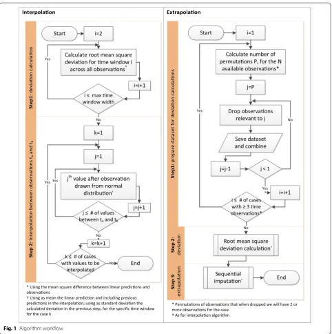
Methods

is used for extrapolations, if requested. The algorithm workflow for both interpolation and extrapolation is pre-sented in Fig. 1. User defined MNAR assumptions are also allowed, under which values can be imputed through either interpolation or extrapolation. The command is computationally demanding and can take a long time to run for very large populations, especially when both inter-polations and extrainter-polations are requested. Time-win-dows can be in years, months or even days, provided data completeness is reasonable. For example, in UK primary

care databases, BMI is routinely recorded for people with certain chronic conditions at least once every year, since physicians are incentivized to measure it. In a clinical trial BMI may be recorded on a weekly basis and hence a much smaller time-window for analysis may be desirable.

Cleaning

In the standard cleaning approach, the algorithm simply sets values below 8 or above 210 to missing. BMI values outside this range are extremely unlikely, Interpolaon

Step1:

deviaon calculaon

Extrapolaon

Step1:

prepare dataset for deviaon calculaons

Step 2 : deviaon Step 3 : extrapolaon Step 2 :

Interpolaon between observaons t

a

and

tb

Calculate root mean square deviaon for me window i

across all observaons*

i ≤ max me window width

i=2

Yes

k=1 No

k ≤ # of cases with values to be

interpolated j=1

Yes j

th _{value aer observaon} drawn from normal

distribuon†

* Using the mean square difference between linear predicons and observaons

† Using as mean the linear predicon and including previous predicons in the interpolaon; using as standard deviaon the calculated deviaon in the previous step, for the specific me window for the case k

j ≤ # of values between ta and tb

Yes No Start End No i=1 Yes

* Permutaons of observaons that when dropped we will have 2 or more observaons for the case

† As for interpolaon algorithm Start

i ≤ # of cases with ≥ 3 me observaons* i=i+1

j=j+1

k=k+1

Calculate number of permutaons P, for the N

available observaons*

j=P

Drop observaons relevant to j

Save dataset and combine

j < 1 j=j-1

No

Yes i=i+1

No

Root mean square deviaon calculaon†

Sequenal

imputaon† End

across all ages [15]. If height and weight are provided, similar range restrictions are applied, between 0.81 and 2.3 m and 15–500 kgs (if age is also provided the lower limits only apply to individuals aged 10 or over). The upper and lower values threshold can be edited by the user.

Under the more advanced regression-based cleaning setting, weight and height values, when available, are used to compute a BMI score for comparison against the recorded BMI values. First, height observations are used to estimate the median height value. Since we assume height to be constant over time (unless age is provided, in which case the approach is limited to those aged 18 or over), height is replaced with the median value in all time points. Next, potentially more reliable BMI values are calculated using the ‘corrected’ height value and the available weight values (again, taking age into account if provided). As in standard cleaning, BMI values are set to missing if they are outside the [8, 210] range.

In the final step of the regression-based cleaning (and first if weight and height are not provided, for example when the variable of interest is not BMI), a linear regres-sion of time on the variable oif interest is executed, for each individual with three or more observations. We run a separate ordinary least squares model for each indi-vidual, analogous to some extent to previously proposed random-effects modelling [16]. For time points where the ratio of absolute model residual value (observation minus prediction) over the observation is higher than 0.5 (50%), the observation is assumed to be unrealistic and is dropped. The value rejection threshold can be set by the user in the (0, 10] range.

Interpolation

The main feature of the algorithm is imputation of miss-ing values between observations, for each individual. Although the command and methods were originally developed for BMI imputation, they should be relevant to any variable with very low individual-level variability.

In the first step, available observations are used to quantify the error of predictions using the ipolate

command. For each possible distance between time points, we assume existing observations are missing and impute them using ipolate. Subtracting each estimate from the actual observation we calculate the root mean square deviation, which we aggregate across all cases for each time-window width. Assuming a time-window width i, taking values between 2 (e.g. between time points 1 and 3, 2 and 4 etc) and k−1, if k is the number of time points:

(1)

irmsdi= 1 n n

j=1

(pred_ij−obsij)2

where n is the total number of cases for which a compari-son is possible, across individuals and time-windows of size i. For example, assuming 5 time points, irmsd2 is

cal-culated across all patients with complete observations for time points 1–3, 2–4 and 3–5: values for time points 2, 3 and 4, respectively, are assumed to be missing and are estimated and then compared to the observed values as described by (1). In other words, the root mean square deviation is calculated pooled across all possible time windows (of a specific width) and all individuals.

The second step involves the actual imputation of miss-ing values, usmiss-ing interpolation. For each individual, any observations that can be interpolated are identified. For each set of values to be imputed, between two observa-tions in time points tα and tβ, the time-window width is identified and linked to the respective root mean square deviation calculated in step 1. Next, the group of values is imputed sequentially, starting from time point tα+1. For

tα+1, the value to be imputed is randomly drawn from

N(mvtα+1,irmsdtβ−tα), where mvtα+1 is the interpolation

value provided by the ipolate command for time point

tα+1 using tα and tβ values. The next time point for which a value is imputed is tα+2 (assuming tβ−tα>2 ), ran-domly drawn from N(mv′

tα+2,irmsdtβ−tα), where mv

′ tα+2

is the interpolation value provided by the ipolate com-mand for time point tα+2 using tα+1 and tβ values. In other words, for each imputed value, the immediately pre-vious value is always taken into account, whether observed or imputed. This approach allows for imputed values that do not fluctuate unrealistically around a mean but rather simulate trends of increasing, decreasing or stable values between observations. The more imputed variables are generated, the more of these possible trends are simulated.

Extrapolation

The algorithm will also allow missing values for an indi-vidual to be extrapolated, in a process based on the

ipolate or regress commands. The extrapolation process involves three steps.

In the first step, the available dataset is edited and reshaped to allow for the comparison of predictions with observations, for all possible extrapolations. For exam-ple, if an individual’s observations are available for time points tα, tβ, tγ and tδ, the algorithm will ‘drop’ values to

generate subsets on which the comparisons will take place. In this case it will generate four subsets by drop-ping tα, tα and tβ, tδ, tδ and tγ, allowing the evaluation of

The temporary file is then used to calculate root mean square deviation estimates, in a similar way as for inter-polation, but in this case they are much larger (since the

The _mibmi command Syntax

methods we use to empirically quantify deviation are less accurate). Users can choose either an ipolate or a computationally more expensive regress based esti-mation for all the values that were ‘dropped’ in the previ-ous step, with the former using the closest two and the latter using all available observations. For each possible distance i between the ‘dropped’ value to be imputed and the closest observation, the root mean square deviation is estimated using (1). In this case, however, we call it

ermsdi with n in the formula being the total number of

cases in the temporary file, for which a comparison is possible for time distance i.

In the last step, for each individual, the missing values that can be estimated using extrapolation are identified and linked to the respective root mean square devia-tion calculated in the previous step. As with interpola-tion, extrapolation values are imputed sequentially for each individual, starting from the time point closest to an observation. Assuming an observation exists for time point tα and an extrapolation can be calculated for tα+1 , the value to be imputed will be randomly drawn from

N(mvtα+1,ermsd1), where mvtα+1 is the extrapolation

value provided by ipolate or regress for time point

tα+1. Assuming tα+2 can be extrapolated, it is ran-domly drawn from N(mvt′α+2,ermsd2), where

′ mvtα+2 the

extrapolation value provided by ipolate or regress

for time point tα+2, but including the imputed value for

tα+1 in the process. The algorithm continues sequen-tially and imputes values for all time points where an extrapolations is possible, for each individual, simulating realistic variable trends (as many for each individual as the number of variables to be generated in the imputa-tion process). Draws for both interpolaimputa-tion and extrapo-lation are effectively constrained to acceptable values in the [8, 210] range, although in our experience this con-straint should never have to be invoked for interpolations and only very rarely for extrapolations. It should also be noted that each drawn interpolation or extrapolation is assumed to be exact, within the specific dataset, and only through a multiple imputation process will the uncer-tainty in the estimate be fully captured.

Variables

The command requires three variables to be provided, in the following order: the unique within time individual identifier (varname1); a linear time variable to define monthly, yearly or other time-windows (varname2); and the main variable of interest, usually the BMI (

var-name3). An optional variable with the age in years can

also be provided (varname4), which is used in the sim-ple cleaning process, if requested. Also note that the data needs to be in long rather than wide format, in relation to time. A backup variable for the original variable of inter-est is created in _varname3.

Options Cleaning

weight(varname) Weight in kilograms. If provided along with height, both variables will be used to correct BMI and/or height and weight observations. Only rel-evant for BMI imputation.

height(varname) Height in metres. If provided along with weight, both variables will be used to correct BMI and/or height and weight observations. Only relevant for BMI imputation.

clean Standard cleaning option requested to set unre-alistic values to missing (default is >210 or <8). Assuming the variable of interest is BMI, if weight and height have been provided they are also cleaned at this stage, taking age into account if it has been provided.

interest is not BMI, involves running a regression model for each subject to identify unrealistic changes in BMI and set them to missing. The threshold over which the observations are set to missing is set with the xclnp(#)

option.

xclnp(#) Threshold for regression cleaning, defined as absolute residual value (i.e. observed minus prediction) over observed value. The default value is 0.5 (i.e. 50%).

xnomi By default the command is a multiple tion command. This option suppresses multiple imputa-tions and hence allows the command to be used solely for cleaning.

xsimp By default the command is a multiple imputation command. This option suppresses multiple imputations and allows simple imputation, with no standard errors calculated and implemented in either intrapolations or extrapolations. It can be issued with the ixtrapolate

or rxtrapolate options

Multiple imputation

minum(#) Number of multiple imputations. The default is five.

ixtrapolate Requests extrapolation (in addition to interpolation), using the ipolate command. Standard errors for ipolate predictions are calculated (for vari-ous time-windows), by removing observed BMI values and calculating model performance for them. The ipo-late command (with the extrapolation option) is then used to sequentially impute extrapolated values: start-ing from the time points closest to the observed val-ues and moving further away. At each stage, valval-ues are drawn from a normal distribution the mean for which is provided by the ipolate command and its standard deviation is the standard error for the predictions for the respective time-window.

rxtrapolate Requests extrapolation (in addition to interpolation), using the regress command. Standard

errors for regress predictions are calculated (for various time-windows), by removing observed BMI values and calculating model performance for them. The regress command is then used to sequentially impute extrapolated values: starting from the time points closest to the observed values and moving fur-ther away. At each stage, values are drawn from a nor-mal distribution the mean for which is provided by the

ipolate command and its standard deviation is the standard error for the predictions for the respective time-window.

imnar(#) Missing not at random (MNAR) assumption for interpolated values. Increases or decreases the pre-dictions by the value specified, in the [−50,+50] range

but within the logical range for BMI.

xmnar(#) Missing not at random (MNAR) assumption for extrapolated values. Increases or decreases the pre-dictions by the value specified, in the [−50,+50] range

but within the logical range for BMI.

pmnar Indicates that a percentage change, rather than an absolute value increase/decrease, is to be used for the MNAR mechanism(s). If this option is specified, options imnar(#) and xmnar(#) will accept values in the [−0.9, +0.9] range, indicating a percentage change between −90 and 90%. Users should be aware that increases and decreases are not symmetrical under this option.

milng Requests the multiple imputations dataset in

mlong format instead of wide, the default.

Other

lolim(#) Lower value threshold below which observa-tions are dropped when using option clean and imputa-tions are constrained. The default value, for adult BMI, is set to 8.

are constrained. The default value, for adult BMI, is set to 210.

seed(#) Set initial value of random-number seed, for the simulations. The default is 7. See set seed.

nodi Do not display progress. Not recommended since imputation can take a very long time for large databases.

Saved results

The mibmi command does not return any scalars but an edited dataset, mi compatible if imputations are per-formed. In that case, additional variables are included. The mi standard variable _mi_miss includes binary information on whether values are missing or not. Vari-ables _mi_ipat and _mi_xpat flag patients for which at least one value has been interpolated or extrapolated, respectively (the latter is only present if extrapolations have been requested). Assuming the default mi wide

format is used, imputed variables are available in the usual Stata format _i_varname3, including observed and imputed values (the number of variables is defined by

minum(#)). Finally, _i_iinfo and _i_xinfo, if extrapola-tions are requested, include information on the imputed observations and the validity of the imputed values for the respective variable, i.e. they flag whether the imputa-tion process would have provided a value outside the pre-defined logical range and had to be corrected by setting to the minimum or maximum allowed. Such a scenario

is extremely unlikely for interpolations and _i_iinfo variables do not really vary (zero for all imputed val-ues, missing for observations). However, it does happen for extrapolations, although rarely, and on occasion the

_i_xinfo variables include non-zero values. This seems

to be more likely with the default and faster ipolate

approach, which only accounts for two observations during the prediction process and is more sensitive to extreme or incorrect values.

Example

We present BMI characteristics for two representa-tive time points: 2009/10 (year 10) and 2011/12 (year 12), the last year of the study. At least one BMI meas-urement is available for 2605 of 3252 eligible individu-als in 2009/10 (80.1%) and for 2315 of 3487 in 2011/12

The analysis on the original dataset indicates that the relationship between BMI and polypharmacy is very weak and non-significant. Next, we only use the simple

A handful of extreme BMI observations were set to missing but further corrections have been performed, based on available weight and height measurements. We

Analysis on the (simply) cleaned datasets suggests there is statistically significant relationship between BMI and polypharmacy. Next, we go one step further with the

A few more values are dropped due to regression clean-ing (with a low 20% threshold defined by the xclnp(#)

We focus on the characteristics of variable _1_BMI, but the imputed cases (not imputed values) are identical across all three variables. For 2009/10 (year 10) and each imputation set, the algorithm imputed 179 observations (2780 now, compared to 2601 when only using simple and advanced cleaning). Unsurprisingly, no values are interpolated for the last time point, 20111/12 (year 12). Three new variables provide information on the interpo-lation process: _mi_miss flags all missing BMI observa-tions; _1_iinfo flags cases where interpolated values for _1_BMI were unrealistic and had to be constrained (in this example there were none, amongst the 1152 that were imputed); and _mi_ipat flags all patients for whom at least one observation was interpolated, at any point in time. The role of _mi_ipat is to allow users

to easily obtain the number of patients with at least one interpolation:

Finally, we can use all four aspects of mibmi with the original dataset: simple and advanced cleaning, interpo-lation and extrapointerpo-lation.

Again, we focus on the characteristics of variable _1_ BMI. For 2009/10 (year 10) and each imputation set, the algorithm now imputed 410 observations, of which 213 are extrapolations (3011 now, compared to 2780 with

interpolation and cleaning and 2601 with cleaning only). For the last time point, 20111/12 (year 12), 416 values were imputed with extrapolation (2723 now, compared to

amongst the 1183 extrapolated values); and _mi_xpat

flags all patients for whom at least one observation was interpolated, at any point in time (with a role similar to _mi_ipat, allowing users to obtain the number of patients with at least one extrapolation).

Results from a multiple imputation analysis on the final dataset obtained with mibmi were similar to

and extrapolated values separately, since the underly-ing principles in their imputations are different, for

mibmi at least. Performance for interpolated values appears to be similar while twofold performs better for extrapolations.

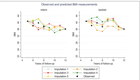
In the second assessment, which focused on interpola-tion, we again randomly selected 10,000 people but this time with 5 or more BMI measurements over the study period. Next, for each individual, we randomly set three concurrent BMI observations to missing but ensuring these were observations that would be imputed as inter-polations under the mibmi algorithm (i.e. observations were available both before and after these ‘missing’ val-ues, for all patients). As before, we used mibmi, with both simple and multiple imputation options, and two-fold with the five available biological parameters for the multiple imputations and we aggregated to obtain mean errors. Results are presented in Table 2, both overall and for each of the three sequential observations that we set to missing. Performance was better with mibmi, espe-cially for the second time point, the one furthest away from observations. A prediction example using a single patient is presented in Fig. 2.

These results indicate that, for interpolating BMI val-ues, there is little useful information in other biological parameters and the additional effort of obtaining them is not justified. The mibmi algorithm generates realistic linear or curvilinear trends for BMI over time and the higher computational complexity pays off more as the number of concurrent missing values increases. How-ever, for extrapolating BMI values, performance is bet-ter with the twofold fully conditional specification algorithm and use of all biological parameters, at least when only two observations per individual are avail-able. In such a scenario, each extrapolation is based on an individual-level model that uses only two observations Performance

To assess the performance of mibmi, in relation to the recently presented twofold algorithm, we used a ver-sion of the diabetes patients dataset we presented previ-ously. For this exercise, the dataset included additional information on HbA1c (glucose), systolic and diastolic blood pressure and total cholesterol. First, we applied the

mibmi algorithm with the simple and regression clean-ing options to obtain a more reliable measure for BMI, thus not allowing extreme and erroneous values to affect the comparison.Then we performed two assessments of performance, when one or three values were miss-ing between two observations for each individual. We did not choose to evaluate through a simulations frame-work since the assumptions under which we would have simulated the data would be critical to the analyses and the evaluation could be seen as self-fulfilling proph-ecy. Rather, we used real data to assess deviations from observations. Therefore, we could not evaluate the per-formance (e.g. coverage, power) of the inferential models since the true effects and associations were unknown.

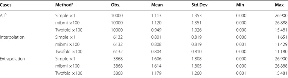
In the first assessment, we randomly selected 10,000 people with 3 or more BMI measurements over the study period and we randomly set one BMI observation per person to missing. We then used mibmi, with both sim-ple (×1) and multiple imputation options (×100), and twofold in which we used all five available biological parameters for the multiple imputations. Under a mul-tiple imputations approach, we obtained 100 BMI vari-ables with imputed values, for each algorithm. Each set was then aggregated and we obtained their mean value for each of the 10,000 ‘missing’ observations. Finally, these aggregates, as well as the simple imputation BMI from mibmi, were compared to the ‘true’ BMI values to calculate absolute mean differences (mean error). Table 1 presents the overall results and for interpolated

Table 1 Mean errors between observed and imputed BMI values, one missing value per individual

a _{Simple refers to a single imputation that ignores variability in the observations (option xsimp); mibmi refers to the default multiple imputation approach with the}

command and 100 imputations; twofold refers to the twofold algorithm described in the paper and 100 imputations

b _{All refers to both interpolations (between observations imputations) and extrapolations (not between observations imputations)}

Cases Methoda _{Obs. Mean Std.Dev Min Max}

Allb _{Simple ×1 10000 1.113 1.353 0.000 26.900}

mibmi ×100 10000 1.120 1.351 0.000 26.888

Twofold ×100 10000 0.949 1.026 0.000 15.481

Interpolation Simple ×1 6132 0.801 0.819 0.000 11.651

mibmi ×100 6132 0.808 0.819 0.001 11.429

Twofold ×100 6132 0.804 0.810 0.000 11.180

Extrapolation Simple ×1 3868 1.606 1.808 0.000 26.900

mibmi ×100 3868 1.614 1.805 0.000 26.888

which, unsurprisingly, can generate extreme values in some cases. Although the accuracy of extrapolation predictions might improve for mibmi as the number of available observations increases, performance with the

twofold algorithm should remain better.

Discussion

In this paper we presented mibmi, a new command for cleaning and imputing BMI values, or other variables with very low individual-level variability, in longitudi-nal settings. Using a pseudo-anonymised dataset from

20

24

28

32

36

40

44

BMI

4 6 8 10 12

Years of follow-up mibmi

20

24

28

32

36

40

44

BMI

4 6 8 10 12

Years of follow-up twofold Observed and predicted BMI measurements

Imputation 1 Imputation 2 Imputation 3 Imputation 4 Imputation 5 Observed Fig. 2 Predictions example for a single patient

Table 2 Mean errors between observed and imputed BMI values, three sequential missing values per individual (interpo-lation only)

a _{Simple refers to a single imputation that ignores variability in the observations (option xsimp); mibmi refers to the default multiple imputation approach with the}

command and 100 imputations; twofold refers to the twofold algorithm described in the paper and 100 imputations

b _{All refers to aggregates across all three time points}

Cases Methoda _{Obs. Mean Std.Dev Min Max}

Allb _{Simple ×1 30,000 0.980 1.002 0.000 16.017}

mibmi ×100 30,000 0.989 1.004 0.000 16.034

Twofold ×100 30,000 1.137 1.155 0.000 18.318

Time point 1 Simple ×1 10,000 0.935 0.945 0.000 9.829

mibmi ×100 10,000 0.943 0.947 0.000 9.779

Twofold ×100 10,000 1.094 1.114 0.000 18.318

Time point 2 Simple ×1 10,000 1.059 1.068 0.000 16.017

mibmi ×100 10,000 1.069 1.071 0.000 16.034

Twofold ×100 10,000 1.234 1.231 0.000 17.126

Time point 3 Simple ×1 10,000 0.947 0.984 0.000 10.645

mibmi ×100 10,000 0.955 0.985 0.000 10.538

the Clinical Practice Research Datalink we described the command’s cleaning and imputation functions over a few examples and we also assessed its performance. The com-mand is available to download from the ssc archive by typing ssc install mibmi within Stata. Alternatively read-ers can automatically download from the first author’s personal web page by typing net fromhttp://statanalysis. co.uk within Stata and following the instructions.

We argue that mibmi can be a useful tool for researchers who wish to use longitudinal values for BMI or other variables with very low individual-level vari-ability, in descriptive or inferential analyses. The com-mand is fully compatible with the mi family of Stata and we incorporated numerous features to allow for flexibility in the imputation process, allowing the user to assume certain MNAR mechanisms. The same pro-cesses could be used for imputation of other param-eters, providing one can assume very strong correlation over time and linearity.

The algorithm’s advantage is its ability to provide multiple datasets with imputed values for the vari-able of interest when no other information is availvari-able, except for an individual identifier and time. For inter-polations, BMI performance was overall better than in other multiple imputation approaches that use addi-tional biological data. Because of the command’s indi-vidual by indiindi-vidual approach, the interpolation and, especially, extrapolation processes are computationally expensive and, for very large datasets (of hundreds of thousands of patients), the command can take weeks to execute. When multiple imputation is selected, we recommend 5 generated datasets. However, the process can be parallelized and for large centralized data repos-itories, like the UK Primary Care Databases (CPRD, THIN, QResearch), mibmi could be applied once at a high level and the imputed BMI values distributed to users when requested, on a protocol-by-protocol basis. The algorithm will effectively ignore patients with fewer than 2 BMI values over time and hence research-ers are unlikely to have a complete final dataset to ana-lyze. Also note that users who extrapolate should take care to impute at appropriate times only (e.g. not when age <18).

In the context of BMI imputation, when additional biological information is available (e.g. blood pressure values), we advise its use in conjunction with twofold, especially for extrapolations. In the first step, users can execute mibmi to obtain a more reliable BMI variable through the cleaning options and generate interpolated values for patients with at least two observations over the study period. In the second step they can use the gener-ated variable with the twofold algorithm, to obtain multiple imputations for BMI and other variables.

Abbreviations

BMI: body mass index; CPRD: Clinical Practice Research Datalink; EMR: elec-tronic medical records; MAR: missing at random; MCAR: missing completely at random; MNAR: missing not at random; THIN: the health improvement network; UK: United Kingdom.

Authors’ contributions

EK designed and developed the command and wrote the manuscript. RP, DR and DAS critically commented onboth the manuscript and the functionality of the command. All authors read and approved the final manuscript.

Author details

1 _{NIHR School for Primary Care Research, University of Manchester, Williamson}

Building, Oxford Road, Manchester M13 9PL, UK. 2 _{Farr Institute for Health}

Informatics Research, University of Manchester, Vaughan House, Portsmouth Street, Manchester M13 9GB, UK. 3 _{Centre for Pharmacoepidemiology & Drug}

Safety, University of Manchester, Stopford Building, Oxford Road, Manches-ter M13 9PL, UK. 4 _{Centre for Biostatistics, University of Manchester, JMF}

Build-ing, Oxford Road, Manchester M13 9PL, UK.

Acknowledgements Not applicable.

Competing interests

The authors declare that they have no competing interests.

Availability of data and materials

The command is freely available to download. We are not allowed to share CPRD data.

Consent for publication Not applicable.

Ethics and consent statement

This study is based on data from the Clinical Practice Research Datalink (CPRD) obtained under licence from theUK Medicines and Healthcare products Regula-tory Agency. However, the interpretation and conclusions contained inthis paper are those of the authors alone. The study was approved by the independ-ent sciindepend-entific advisory committee(ISAC) for CPRD research (reference number: 16 115R). No further ethics approval was required for the analysis ofthe data.

Funding

This study was funded by the National Institute for Health Research (NIHR) School for Primary Care Research(SPCR), under the title ‘An analytical frame-work for increasing the efficiency and validity of research using primarycare databases’ (Project no. 211). This paper presents independent research funded by the National Institute forHealth Research (NIHR). The views expressed are those of the authors and not necessarily those of the NHS, theNational Insti-tute for Health Research or the Department of Health. In addition, MRC Health eResearch CentreGrant MR/K006665/1 supported the time and facilities of one investigator (EK).

Received: 3 May 2016 Accepted: 28 December 2016

References

1. Silverman SL. From randomized controlled trials to observational studies. Am J Med. 2009;122(2):114–20. doi:10.1016/j.amjmed.2008.09.030. 2. Kontopantelis E, Doran T, Springate DA, Buchan I, Reeves D. Interrupted

time-series analysis: a regression based quasi-experimental approach for when randomisation is not an option. BMJ. 2015;350:h2750.

3. Rubin DB. Multiple imputation after 18+ years. J Am Stat Assoc. 1996;91(434):473–89.

4. Carpenter JR, Kenward MG, Vansteelandt S. A comparison of multiple imputation and doubly robust estimation for analyses with missing data. J R Stat Soc: Series A (Statistics in Society). 2006;169(3):571–84. 5. Tang L, Song J, Belin TR, Unützer J. A comparison of imputation methods

• We accept pre-submission inquiries

• Our selector tool helps you to find the most relevant journal • We provide round the clock customer support

• Convenient online submission • Thorough peer review

• Inclusion in PubMed and all major indexing services • Maximum visibility for your research

Submit your manuscript at www.biomedcentral.com/submit

Submit your next manuscript to BioMed Central

and we will help you at every step:

6. Saha C, Jones MP. Bias in the last observation carried forward method under informative dropout. J Stat Plan Inference. 2009;139(2):246–55. 7. Lee KJ, Carlin JB. Recovery of information from multiple imputation: a

simulation study. Emerg Themes Epidemiol. 2012;9:3.

8. Potthoff RF, Tudor GE, Pieper KS, Hasselblad V. Can one assess whether missing data are missing at random in medical studies? Statl Methods Med Res. 2006;15(3):213–34.

9. Schafer JL, Graham JW. Missing data: our view of the state of the art. Psychol Methods. 2002;7(2):147–77.

10. Groenwold RHH, Donders ART, Roes KCB, Harrell FE Jr, Moons KGM. Deal-ing with missDeal-ing outcome data in randomized trials and observational studies. Am J Epidemiol. 2012;175(3):210–7. doi:10.1093/aje/kwr302. 11. Nevalainen J, Kenward MG, Virtanen SM. Missing values in longitudinal

dietary data: a multiple imputation approach based on a fully conditional specification. Stat Med. 2009;28(29):3657–69.

12. Welch C, Bartlett J, Petersen I. Application of multiple imputation using the two-fold fully conditional specification algorithm in longitudinal clini-cal data. Stat Med. 2014;33(21):3725.

13. Welch CA, Petersen I, Bartlett JW, White IR, Marston L, Morris RW, Nazareth I, Walters K, Carpenter J. Evaluation of two-fold fully conditional specifica-tion multiple imputaspecifica-tion for longitudinal electronic health record data. Stat Med. 2014;33(21):3725–37. doi:10.1002/sim.6184.

14. Engels JM, Diehr P. Imputation of missing longitudinal data: a comparison of methods. J Clin Epidemiol. 2003;56(10):968–76.

15. Royal College of Paediatrics and Child Health: School Age Charts and Resources. http://www.rcpch.ac.uk/child-health/research-projects/ uk-who-growth-charts/uk-growth-chart-resources-2-18-years/school-age

16. Welch C, Petersen I, Walters K, Morris RW, Nazareth I, Kalaitzaki E, White IR, Marston L, Carpenter J. Two-stage method to remove population- and individual-level outliers from longitudinal data in a primary care database. Pharmacoepidemiol Drug Saf. 2012;21(7):725–32. doi:10.1002/pds.2270. 17. Kontopantelis E, Springate DA, Reeves D, Ashcroft DM, Rutter M, Buchan