Optimising resilience : at the edge of computability

Optimising Resilience: at the Edge of Computability

Massimiliano Vasile

Aerospace Centre of Excellence

Department of Mechanical and Aerospace Engineering

University of Strathclyde

Published in Mathematics Today, vol. 53, no. 5, pp. 231-234, October 2017

1

Handling the Unknown

In the past two decades, Uncertainty Quantification (UQ), as the science that studies how to quantify and reduce the effect of uncertainty on the response of a system or process, has grown significantly, finding practical application in many areas of engineering. UQ lives at the intersection of applied mathematics, probability, statistics, computational science and engineering and has become a key enabling technology in the design and control of complex engineering systems.

UQ is of key importance to improve reliability and resilience of engineering systems but presents considerable theoretical and computational challenges. The theoretical challenge is to capture and model different types of uncertainty. It is customary to classify uncertainty in aleatory, or irreducible, and epistemic, or reducible, where the former is due to inherent probabilistic variability while the latter is due to a contingent lack of knowledge. This classification, however, is not fully descriptive and does not provide any information on the source of uncertainty.

The sources of uncertainty can be many. We can roughly group them in three categories: uncertainty coming from manufacturing and control processes (including human factors), uncertainty coming from measurement processes (maybe the most well understood) and uncertainty coming from our ability to model and simulate natural phenomena. Following this grouping we can further divide the source of uncertainty in:

• Structural (or model) uncertainty. This is a form of epistemic uncertainty on our ability to correctly model natural phenomena, systems or processes. If we accept that the only exact model of Nature is Nature itself, we also need to accept that every mathematical model is incomplete. One can then use an incomplete (and often much simpler and tractable) model and account for the missing components through some model uncertainty.

• Experimental uncertainty. This is a form of aleatory uncertainty, probably the easiest to understand and model, if enough data are available, on the exact repeatability of measurements.

• Geometric uncertainty. This is a form of aleatory uncertainty on the exact repeatability of the manufacturing of parts and systems.

• Parameter uncertainty. Parameter uncertainty can be either aleatory or epistemic and refers to the variability of model parameters and boundary conditions.

• Numerical (or algorithmic) uncertainty. Numerical uncertainty, also know as numerical errors, refers to different types of uncertainty, related to each particular numerical scheme, and to the machine precision (including clock drifts).

• Human uncertainty. This is a difficult uncertainty to capture as it has elements of both aleatory and epistemic uncertainty and is dependent on our conscious and unconscious decisions and reactions. This uncertainty includes the possible variability of goals and requirements due to human decisions.

challenge. The growing popularity of UQ in the past two decades is in part due to the increase in computational resources. Although many significant advances in computational methods allow us to treat problems before intractable, still many UQ problems remain NP-complex. Furthermore, the computational cost of simulations, in some areas of engineering (like computational fluid dynamics) or the time and resources required to perform experiments make the collection of large data sets prohibitive.

Capturing and quantifying uncertainty is only part of the challenge. The other part is to do something with it so that reliability, robustness and ultimately resilience are maximised while achieving an optimal level of performance. This is well understood in estimation and control theory when the control action closes the loop with the estimation of the current state. In Multi-disciplinary Design Optimisation this loop combines UQ with optimisation. This close-loop pairs a problem whose complexity grows exponentially with the number of dimensions, with another problem that is often NP-complex in nature.

2

Modeling and Propagating Uncertainty

The first question on the quantification of uncertainty is how to model uncertainty. As explained in the previous section one obvious choice is to define an uncertainty space and associate a family of probability distributions to all stochastic quantities. With reference to the different sources of uncertainty experimental, geometric and parameter uncertainties all can be well captured (in most of the cases) with an appropriate mixture of probability distributions. The other types of uncertainty might require other models.

It is customary to divide methods for uncertainty quantification in intrusive and non-institutive. Non intrusive techniques are sampling based methods that work with generic models in the form of black-box codes. They have little requirements on the coding of the models or on their regularity. Non-intrusive can be used to capture model uncertainty by identifying missing components from the assimilation of experimental data and measurements. The most obvious form of non-intrusive approach is to use Monte Carlo Simulations and then reason on the outcome. Despite the easiness of this approach, it is, generally, the one with the highest computational cost. Furthermore, it does not offer a model as direct outcome of the simulations. For these reasons, more sophisticated techniques have been developed in recent times, most of which are based on a clever sampling scheme and a functional representation of the outcomes.

A particular sampling scheme, called Unscented Transformation (UT), was introduced by [Julier et al. (1995)] to reduce the cost of non-linear sequential filtering. The Unscented Transformation works on the underlying hypothesis that one can well approximate the posteriori covariance by propagating a limited set of optimally chosen samples, called sigma points. The UT allows one to reduce the number of samples to 2n+1, with nthe number of dimensions, and obtain a good approximation of the first two statistical moments. On the other hand the sampling scheme strongly relies on the symmetry of the a priori distribution and provides, anyway, only a local quantification in a neighborhood of a reference point.

A more global representation is offered by the so-called Polynomial Chaos Expansions (PCEs) [Wiener (1938)]. Iff is the quantity of interest PCEs provide a representation of the distribution of f in the form:

φ(ξ) =

_∑

cIαI(ξ)

whereξ ∈Ω⊂Rn is the vector of uncertain parameters, m is the maximum degree of the polynomial

expansion and<αI(ξ)>is a multivariate base of orthonormal polynomials. The unknown coefficients can be found by various methods such as least-squares regression or pseudo-spectral collocation. PCEs allow one to use different polynomial kernels depending on the input distribution. PCEs are popular in Computational Fluid Dynamics and have found recent applications also in astrodynamics [Jones et al. (2013),

Vetrisano and Vasile (2016)]. Fig. 1shows the distribution of the velocity vector of a spacecraft along a trajectory from a Libration Point Orbit (in the Earth-Moon system) to the Moon. Fig.1a presents the result of an MC simulation with one million samples while Fig.1b is the result of a PCE of degree 6 that uses only 28,000 samples (see [Vetrisano and Vasile (2016)] for more details). Complex multimodal distribution can be captured also with Gaussian Mixture Models (GMM) [Giza et al. (2009)] or adaptive High-Dimensional Model Representations [Kubicek et al. (2015)].

Intrusive techniques cannot treat computer codes as a black box. They require full access to the mathematical model and computer code and introduce a modification of the code and model itself. The main advantage of intrusive methods lays in the better control of the propagation uncertainty trough the model. One example is the intrusive counterpart of PCEs [Wiener (1938)].

(a) (b)

Figure 1: Velocity distribution for a Libration Point to Moon trajectory: a) Monte Carlo Simulation with 1e6 samples, b) PCE of degree 6 with 28,000 sample.

spacePd,n(α) =<αI(ξ)>whereξ ∈Ω⊂Rn,I= (i1, . . . ,in)∈Nn+and|I|=∑nj=1ij≤d, is the space

of polynomials in theα basis up to degreed inn variables. This space can be equipped with a set of elementary arithmetic operations, generating an algebra on the space of polynomials such that, given two elementsA(ξ),B(ξ)∈Pd,n(α) approximating any two real multivariate functions fA(ξ)and fB(ξ), it

stands that

fA(ξ)⊕fB(ξ)∼A(ξ)⊗B(ξ), (1)

where⊕ ∈ {+,−,·, /} and⊗is the corresponding operation inPn,d(αi). This allows one to define the

algebra(Pd,n(αi),⊗), of dimension dim(Pd,n(αi),⊗) =Nn,d= d+_nn, the elements of which belong to

the polynomial ring innindeterminatesR[ξ]and have degree up tod. Each elementP(ξ)of the algebra, is

uniquely identified by the set of its coefficientsp∈RNn,d _{such that}

P(ξ) =

_∑

pIαI(ξ). (2)

In the same way as for arithmetic operations, it is possible to define a composition rule in the polynomial algebra and hence the counterpart, in the algebra, of the elementary functions. Differentiation and integration operators can also be defined. By defining the initial conditions and model parameters of the dynamics as element of the algebra and by applying any integration scheme with operations defined in the algebra, at each integration step the polynomial representation of the state flow is available. The main advantage of the method is in the control of the trade-off between computational complexity and representation accuracy at each step of integration. Furthermore, sampling and propagation are decoupled, therefore, irregular regions can be propagated with a single integration, provided that a polynomial expression is available. It has been shown that the polynomial algebra approach presents overall good performance and scalability (with respect to the size of the algebra) compared to its non-intrusive counterpart. On the other hand, being an intrusive method, it cannot treat the dynamics as black box. Its implementation requires operator overloading for all the algebraic operations and elementary functions defining the dynamics, making it more difficult to implement than a non-intrusive method. Fig. 2 shows an example of propagation of the uncertainty in the initial conditions of a satellite orbiting the Earth. The figure compares a full Monte Carlo simulation against a single integration of the equations of motion with a Taylor-based algebra (i.e algebra based on an expansion in Taylor polynomials) or with a Chebyshev-based algebra (i.e algebra based on an expansion in Chebyshev polynomials). The figure shows that Taylor diverges as one departs from the estimated state of the satellite. On the contrary, in this case, Chebyshev offers a more stable global representation of the uncertainty space (see [Ortega et al. (2016)] for more details).

2.1

A Question of Imprecision

Figure 2: Propagated uncertainty with Taylor and Chebyshev polynomial algebra.

are acquired on given events, or can derive from subjective probabilities that come from human responses and behaviour. A number of authors argued that classical Bayesian approaches can fail and a different type of approach is required to capture partial or conflicting sources of information. This is the basic motivation for Imprecise Probabilities Theories that extend classical Probability Theory to incorporate imprecision. For example, it is argued that Probability Theory struggles to represent personal indeterminacy and group inconsistency as it does not capture a range of opinions or estimations adequately without assuming some consensus of precise values on the distributions of opinions.

A number of theories have been developed to account for imprecision. Dempster-Shafer evidence theory [Dempster (1967),Shafer (1976)] characterises evidence with discrete probability masses, where Belief-Plausibility pairs are used to measure incertitude. Possibility theory [Dubois (1988)] that represents incertitude with Necessity-Possibility pairs. Walley [Walley (1991)] proposed a coherent lower prevision theory following the work of de Finetti’s subjective probability theory. Families of probability distributions can be modeled with p-boxes or intervals can be incorporated into probability values[Weichselberger (2000)]. Other ways to capture imprecision are offered by random sets[Molchanov (2005)], rough sets[Pawlak (1982)], fuzzy sets[Zadeh (1965)], clouds[Neumaier (2004)] and generalised intervals[Wang (2004)].

2.2

The Unknown Unknowns

In the design of a system, contingency and margins based on historical data are commonly used to cover for the unavoidable growth of resources such as mass, power, cost, etc. Contingency is defined as the difference between the current best estimate (BE) of a resource, or design budget, and its maximum expected value (ME), whereas margin is the difference between the maximum possible value (MP) and maximum expected value of the design budget. Contingency accounts for expected growths due to uncertainties and variability, whereas margins account for unexpected ones due to unknown unknowns. The quantification of contingencies is driven by a predictable model of a stochastic event. The challenge is to model the unknown knowns other than with a margin. The reason is twofold: a) if a maximum possible value is not available from external requirements a sensible margin is hardly defined and b) the maximum possible value can be highly non optimal. In this sense, since the unknown unknown is epistemic in nature, Imprecise Probability Theories might offer an interesting modeling tool.

3

What to Optimise?

interest. In Reliability-Based Optimisation (RBO), instead, the focus is on controlling the violation of some constraints due to uncertainty while optimising a quantity of interest. We can argue that one can combine the concept of robustness and reliability to formulate an optimisation problem that maximises resilience. In this case one should incorporate an element of time as the idea of resilience implies a recovery from shocks or enduring adversities.

3.1

Reliability, Robustness and Resilience

When robustness is of interest, the classical approach is to solve a problem of this form:

min

d E(f(d,ξ))

min d σ

2_(f(d,

ξ)) (RO)

whereE(f(d,ξ))andσ2(f(d,ξ))are respectively, the expected value and the variance (i.e. the first two statistical moments) of the quantity f with respect to the stochastic variablesξ, anddis a vector of design or control parameters. The equivalent RBO formulation is:

min

d E(f(d,ξ))

P(c(d,ξ)≥0)≤ε (RBO)

whereP(c(d,ξ)≥0)is the probability that constraintscare violated due to stochastic variablesξ. In both cases the computation of the statistical moments or the probability of an event is in itself a computationally intensive process. A naive direct application of Monte Carlo simulations is often not an option and one of the methods for UQ described in previous sections are normally used instead.

The use of the first two statistical moments, however, is not a unique choice and in fact might not be the right choice in the case of multimodal distributions, fat tails or imprecision in the uncertainty model. Other quantities have been proposed in the recent past, including Chebyshev inequality, the Value-at-Risk or the conditional Value-at-Risk [Quagliarella and Iuliano (2017)], If we callµthe generic metric to account for the ability of a system to perform within an acceptable envelope under uncertainty andPthe probability measure on the constraint functionsc, we can formulate a resilience problem by introducing a time element in the (RBO) formulation:

max

d µ(d,ξ,t)

P(c(d,ξ,t)≥0)≤ε (RSO)

where the timetaccounts for disruptive events that can lead to a violation of the constraints or a change in performance.

3.2

An Evidence-Based Approach

In the case of imprecision or epistemic uncertainty one formulation that was proposed some years ago[Vasile (2005)], and makes use of Dempster-Shafer Theory (DST) of Evidence, is the following:

max

d Bel(f(d,ξ)<ν)

Pl(c(d,ξ)≥0)≤ε (EBRO)

whereBelandPlare respectively the Belief on the value of f and the Plausibility on the violation of the constraints. The two thresholdνandεcan be given or can be optimised:

max

d Bel(f(d,ξ)<ν)

min

d Pl(c(d,ξ)≥0) (EBRO2)

minν

preimage of f(d,ξ)<ν, of all the focal elements in the power set of the uncertainty spaceΩ. A strategy

to partially avoid the complexity of the calculation ofBelandPlis to study only the worst case scenario, where the worst case for the value off is given by:

ξ=argmax

ξ∈Ω

f(¯d,ξ) (3)

where¯dis given. In the context of robust optimisation this becomes:

d∗=argmin d

max

ξ∈Ω

f(d,ξ) (4)

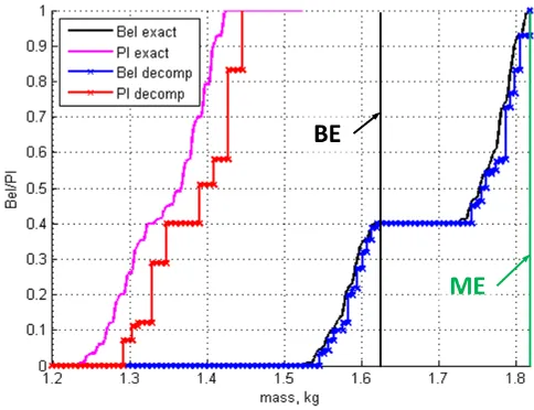
Although the calculation ofd∗and associatedξ∗is a bi-level, zero-sum, global optimisation, the identification of the worst case is a key step also for the solution of (EBRO2) as it provides a limit value forν. An example of this Evidence-Based approach (or Evidence-Based Robust Optimisation) can be seen in Fig.3

where exact and approximated Belief and Plausibility curves are computed for the mass of a cubesat. In this case the design of the cubesat was optimised so that the maximum predictable mass, solution of problem (3) was minimal. In this case the required margin is zero and the ME value is minimal. The same figure shows also the best estimate of the cubesat mass that was provided without accounting for the existing epistemic uncertainty on some system parameters. The calculation of the exact curves required 65536 maximisation and minimisation of the quantity of interest (the mass of the spacecraft) on all focal elements. The approximated curves were calculated with only 0.57% of the computational cost using a decomposition technique proposed in [Alicino and Vasile (2014)]. The gap betweenBelandPlis the degree of ignorance on the probability that the mass of the cubesat is below a given value, while the difference between the mass corresponding toBel=1 and the one corresponding toPl=0 is the minimum range of variability of the mass of the spacecraft due to the current knowledge of the system.

Figure 3: Optimal Belief and Plausibility for the quantification of the mass of a cubesat.

References

[Vetrisano and Vasile (2016)] Vetrisano, M. and Vasile, M. 2016, Analysis of spacecraft disposal solutions from LPO to the Moon with high order polynomial expansions. Advances in Space Research, Vol. 60, No. 1, 01.07.2017, p. 38-56.

[Julier et al. (1995)] Julier, J. K. Uhlmann and Durrant-Whyte, H.F.: A new approach for filtering nonlinear systems, Proceedings of the American Control conference, Seattle, Washington, 1995. DOI: 10.1109/ACC.1995.529783

[Ortega et al. (2016)] Absil, CO, Serra, R, Riccardi, A and Vasile, M 2016, De-orbiting and re-entry analysis with generalised intrusive polynomial expansions. in 67th International Astronautical Congress. Proceedings of the International Astronautical Congress, IAC, Paris, 67th International Astronautical Congress, Guadalajara, Mexico, 26-30 September.

[Giza et al. (2009)] Giza, Daniel and Singla, Puneet and Jah, Moriba, (2009) An Approach for Nonlinear Uncertainty Propagation: Application to Orbital Mechanics, AIAA Guidance, Navigation, and Control Conference, pp. 1–19.

[Wiener (1938)] Wiener, N. (1938). The homogeneous chaos. Amer. J. Math., 897–936.

[Vasile (2005)] 16. Vasile M., Robust Mission Design Through Evidence Theory and Multiagent Collaborative Search. Annals of the New York Academy of Sciences, Vol 1065: pp. 152-173, December 2005.

[Alicino and Vasile (2014)] Alicino, S and Vasile, M 2014, ’Evidence-based preliminary design of spacecraft’ Paper presented at 6th International Conference on Systems & Concurrent Engineering for Space Applications. SECESA 20 dd14, Stuttgart, Germany, 8/10/14 - 10/10/14.

[Dempster (1967)] A. P. Dempster (1967), Upper and lower probabilities induced by a multivalued mapping. Annals of Mathematical Statistics, 38:325–339.

[Shafer (1976)] G. Shafer, A Mathematical Theory of Evidence, Princeton University Press, 1976.

[Walley (1991)] Walley, P.(1991), Statistical reasoning with imprecise probabilities 1st ed. Published 1991 by Chapman and Hall in London, New York.

[Dubois (1988)] Dubois, Didier, Prade, Henri (1988). Possibility Theory. An Approach to Computerized Processing of Uncertainty. Springer 1988.ISBN 978-1-4684-5287-7.

[Weichselberger (2000)] Weichselberger, K (2000). The theory of interval-probability as a unifying concept for uncertainty. International Journal of Approximate Reasoning Volume 24, Issues 2–3, 1 May 2000, Pages 149-170.

[Pawlak (1982)] Pawlak, Zdzisław (1982). "Rough sets". International Journal of Parallel Programming. 11 (5): 341–356. doi:10.1007/BF01001956.

[Zadeh (1965)] L. A. Zadeh (1965) "Fuzzy sets". Information and Control 8 (3) 338–353.

[Molchanov (2005)] Molchanov, I. (2005) The Theory of Random Sets. Springer, New York.

[Neumaier (2004)] , Neumaier, Arnold, (2004). Clouds, Fuzzy Sets, and Probability Intervals, Reliable Computing, 2004,Aug,1, Vol.10, No. 4, pp. 249–272. DOI 10.1023/B:REOM.0000032114.08705.cd.

[Wang (2004)] , Yan Wang (2004),Imprecise probabilities with a generalized interval form. Proc. 3rd Int. Workshop on Reliability Engineering Computing (REC’08).

[Kubicek et al. (2015)] , Kubicek, M. and Minisci, E. and Cisternino, M.(2015), High dimensional sensitivity analysis using surrogate modeling and High Dimensional Model Representation. International Journal of Uncertainty Quantification, 2015.