City, University of London Institutional Repository
Citation:
Fazzolari, F. A., Banerjee, J. R. and Boscolo, M. (2013). Buckling of composite
plate assemblies using higher order shear deformation theory-An exact method of solution.
Thin-Walled Structures, 71, pp. 18-34. doi: 10.1016/j.tws.2013.04.017
This is the accepted version of the paper.
This version of the publication may differ from the final published
version.
Permanent repository link:
http://openaccess.city.ac.uk/14990/
Link to published version:
http://dx.doi.org/10.1016/j.tws.2013.04.017
Copyright and reuse: City Research Online aims to make research
outputs of City, University of London available to a wider audience.
Copyright and Moral Rights remain with the author(s) and/or copyright
holders. URLs from City Research Online may be freely distributed and
linked to.
City Research Online:
http://openaccess.city.ac.uk/
[email protected]
Buckling of Composite Plate Assemblies using Higher Order
Shear Deformation Theory - An Exact Method of Solution
F. A. Fazzolari1,∗, J. R. Banerjee2, M. Boscolo3
City University London, Northampton Square, London EC1V 0HB, UK
Abstract
An exact dynamic stiffness element based on higher order shear deformation theory and extensive use
of symbolic algebra is developed for the first time to carry out a buckling analysis of composite plate
assemblies. The principle of minimum potential energy is applied to derive the governing differential
equations and natural boundary conditions. Then by imposing the geometric boundary conditions in
algebraic form the dynamic stiffness matrix, which includes contributions from both stiffness and initial
pre-stress terms, is developed. The Wittrick-Williams algorithm is used as solution technique to compute
the critical buckling loads and mode shapes for a range of laminated composite plates including stiffened
plates. The effects of significant parameters such as thickness-to-length ratio, orthotropy ratio, number
of layers, lay-up and stacking sequence and boundary conditions on the critical buckling loads and mode
shapes are investigated. The accuracy of the method is demonstrated by comparing results whenever
possible with those available in the literature.
Keywords: Dynamic Stiffness Method, Composite Plates, Buckling, Stiffened Plates, Wittrick-Williams algorithm.
1. Introduction
Aerospace structures are generally made up of thin-walled structures such as plates and shells. Such
structures often experience severe loading conditions. A certain load, referred to as critical load when
applied, the structure suddenly changes its equilibrium configuration. This phenomenon is generally
referred to as buckling instability. The topic is a major design consideration and has continued to be an
important area of research because it represents one of the main reasons for aircraft and other structural
failures. Several methodologies have been developed over the years to solve the problem. A simplified
approach to calculate the ith critical load, is to consider the critical load as the load at which more than
one infinitesimally adjacent equilibrium configurations exist that can be identified with the ith bifurcation
point (Euler’s method) [1]. In a linearized structural stability analysis, the determination of the critical
load leads to a linear eigenvalues problem. The bifurcation method can be successfully used particularly
for plates, when the critical equilibrium configuration shows a slight geometry change as the critical
∗Corresponding author: Tel:+44(0)2070408483, Fax:+44(0)2070408566
Email address: [email protected](F. A. Fazzolari) 1
Ph.D. Candidate, School of Engineering and Mathematical Sciences 2
Professor, School of Engineering and Mathematical Sciences 3
Research Fellow, School of Engineering and Mathematical Sciences *Manuscript
buckling load is reached. However, as explained by Leissa [2], linearized stability analysis is meaningful,
if and only if, the initial in-plane loading does not produce an out-of-plane deformation. Furthermore,
there are many cases in which Euler’s method may fail, in particular when thin-walled structures like
shells exhibit the snap-buckling phenomenon. In such cases, the most general approach, based on the
solution of the complete equilibrium and stability equations [3, 4] is preferred.
Amongst a wide class of methodologies employed to analyze the elastic stability of advanced composite
structures, the dynamic stiffness method (DSM) is probably the most accurate and computationally
effi-cient option. The DSM based on L`evy-type closed form solution for plates [5] is indeed an exact approach
to the solution procedure. Wittick [6] laid the groundwork of the DSM for plates. The basic
assump-tion in this work is that the deformaassump-tion of any component plate varies sinusoidally in the longitudinal
direction. Using this assumption, a stiffness matrix may be derived that relates the amplitudes of the
edge forces and moments to the corresponding edge displacements and rotations for a single component
plate. For the exact DSM, this stiffness matrix is derived directly from the equations of equilibrium
that describe the buckling behavior of the plate. Essentially, Wittrick [6] developed an exact stiffness
matrix for a single isotropic, long flat plate subject to uniform axial compression. His analysis basically
used classical plate theory (CPT). Wittrick and Curzon [7] later extended this analysis to account for
the spatial phase difference between the perturbation forces and displacements which occur at the edges
of the plate during buckling due to the presence of in-plane shear loading. This phase difference was
accounted for by defining the magnitude of these quantities using complex quantities. Wittrick [8] then
extended his analysis further to consider flat isotropic plates under any general state of stress that remains
uniform in the longitudinal direction (i.e., combinations of bi-axial direct stress and in-plane shear). A
method very similar to that described in [6] was also presented by Smith in [9] for the bending,
buck-ling, and vibration of plate-beam structures. Following these developments, Williams [10] presented two
computer programs, GASVIP and VIPAL to compute the natural frequencies and initial buckling stress
of prismatic plate assemblies subjected to uniform longitudinal stress or uniform longitudinal
compres-sion, respectively. GASVIP was used to set up the overall stiffness matrix for the structure, and VIPAL
demonstrated the use of substructuring. Next, Wittrick and Williams [11] reported on the VIPASA
computer code for the buckling and vibration analyses of prismatic plate assemblies. This code allowed
for analysis of isotropic or anisotropic plates using a general state of stress (including in-plane shear).
The complex stiffnesses described in [12] were incorporated in VIPASA, as well as allowances were made
for eccentric connections between component plates. This code also implemented an algorithm, referred
to as the Wittrick-Williams algorithm [13] for determining any buckling load for any given wavelength.
The development of this algorithm was necessary because the complex stiffnesses described above are
transcendental functions of the load factor and half wavelength of the buckling modes of the structure
which make a determinant plot cumbersome and unfeasible. Viswanathan and Tamekuni [14, 15]
pre-sented an exact FSM based upon CPT for the elastic stability analysis of composite stiffened structures
subjected to biaxial in-plane loads. The structure was idealized as an assemblage of laminated plate
elements (flat or curved) and beam elements. Tamekuni, and Baker extended this analysis in [16]
Anisotropic material properties were also allowed. This analysis utilized complex stiffnesses as described
in [12]. The works described in [9, 16, 13] are more or less similar. The differences are discussed in
[11]. Williams and Anderson [17] presented modifications to the eigenvalue algorithm described in [13].
Further modifications presented in [17] allowed the buckling mode corresponding to a general loading
to be represented as a series of sinusoidal modes in combination with Lagrangian multipliers to apply
point constraints at any location on edges. These modifications formed the basis for the computer code
VICON (VIpasa with CONstraints) described in [18]. However, the analysis capability of VICON was
limited to plates analyzed using CPT. Anderson and Kennedy [19] incorporated a first order shear
de-formation plate theory (FSDT) into VICONOPT. A numerical approach to obtain exact plate stiffnesses
that include the effects of transverse shear deformation was presented by them in [19]. It is worth noting
that DSM has been extensively researched by Banerjee [20, 21, 22, 23, 24, 25], amongst a few others
for modal analysis of structures idealized by beam elements based on Euler/Bernoulli, Timoshenko and
associated coupled beam theories. The current paper is partly motivated by these earlier investigations
and the most important contribution made by the authors here is the inclusion of the higher order shear
deformation theory (HSDT) and the use of a systematic symbolic procedure, for the first time, when
developing the DS matrix for laminated composite plates for buckling analysis. This useful extension is
of considerable theoretical and computational complexity as will be shown later. The research is
par-ticularly relevant when analysing thick composite plates for their buckling characteristics. It should be
recognised that Reddy and co-authors [26, 27, 28] have used HSDT for composite plates in a different
context without resorting to the development of the DSM. From a historical prospective HSDT, can be
essentially traced back to third order plate bending theory originally proposed by Vlasov [29] in the late
fifties. His theory was substantiated and extended to laminated composite plates many years later by
Reddy [26] using a variational approach. This is sometimes referred to as Vlasov-Reddy theory (VRT).
Further improvements of this theory can be found in the work of Jemielita [30, 31]. Recently, for the
analysis of anisotropic plates and shells, an advanced hierarchical trigonometric Ritz formulation (HTRF)
based on refined variable kinematics 2D and quasi-3D plate/shell theories has been proposed by Fazzolari
and Carrera for mechanical [32, 33, 34, 35, 36, 37] and multifield [38] problems. Inclusion of HSDT in
the DSM framework will enable buckling analysis of plates with moderate to high thickness-to-width
ratio, in an accurate and computationally efficient manner. The usefulness of HSDT becomes apparent
when analysing composite structures idealized by plates, particularly of thicker dimension, because fiber
reinforced composites have generally very low shear modulii. Extensive results which include validation
and assessment of the effects on critical buckling load of significant parameters such as the thickness to
width (or length) ratio, orthotropy ratio, number of layers, stacking sequence and boundary conditions,
have been obtained, examined and discussed.
2. Theoretical formulation
2.1. Displacement field and governing differential equations
In the derivation that follows, the hypotheses of straightness and normality of a transverse normal
to be a cubic function in the thickness coordinate, and hence the use of higher order shear deformation
theory (HSDT). This development is in sharp contrast to earlier developments based on CPT and FSDT
and no doubt a significant step forward. The deformation pattern through thickness of the plate is shown
in Fig. 1. A laminated composite plate composed ofNl layers is considered in order to make the theory
sufficiently general. The integer k is used as a superscript denoting the layer number which starts from
the bottom of the plate. The kinematics of deformation of a transverse normal using both first order
and higher order shear deformation are shown in Fig. 1. After imposing the transverse shear stress
homogeneous conditions [39, 40] at the top/bottom surface of the plate, the displacements field are given
below in the usual form:
u(x, y, z, t) = u0(x, y, t) +z φx(x, y, t) +c1z 3
φx(x, y, t) +
∂w0(x, y, t)
∂x
v(x, y, z, t) = v0(x, y, t) +z φy(x, y, t) +c1z 3
φy(x, y, t) +
∂w0(x, y, t)
∂y
w(x, y, z, t) = w0(x, y, t)
(1)
where u,v,ware the plate displacement components of the displacement vector,
η=n u v w
oT
(2)
c1 =−34h2 whereasu0, v0,w0 are the displacement components defined on the plate middle surface Ω
in the directions x, y and z. The principle of minimum potential energy is now applied. The variational
statement at multilayer level is:
Nl
X
k=1
δΠk= 0 (3)
where Πk is the total potential energy for the kth layer of the composite plate. The first variation can
be expressed as:
δΠk=δUk+δVk (4)
where δUk is the virtual potential strain energy, δVk is the virtual potential energy due to external
loadings, and assume the following form:
δUk= Z
Ωk Z
zk
δεkT σkdΩkdz, δVk= Z
Ωk Z
zk
δεnlxxσ˜x0+δε
nl yy˜σy0
dΩkdz (5)
the stresses,σ and the strains,εvectors are expressed as follows:
σ=n σxx σyy τxy τxz τyz
oT
, ε=n εxx εyy γxy γxz γyz
oT
(6)
˜
σx0 and ˜σy0 denote the in-plane initial stresses. The non-linear strains ε
nl
xx and εnlyy are approximated
with the Von Karman’s non-linearity:
εnl xx=
1 2 (w, x)
2
εnl yy=
1 2 (w, y)
2
(7)
The subscript T signifies an array transposition and δ the variational operator. Constitutive and
geo-metrical relationships are defined respectively as:
σk = ˜Ckεk ε=
Dη (8)
where ˜Ck is the plane stress constitutive matrix and D is the differential matrix (see Appendix A for
motion are obtained after extensive algebraic manipulation as:
δu0 : A11u0,xx+A12v0,yx+A16(u0,yx+v0,xx) +B11φx,xx+B12φy,yx+B16(φx,yx+φy,xx) +E11c2φx,xx
+E11c2w0,xxx+E12c2φy,yx+E12c2w0,yyx+E16c2φx,yx+E16c2φy,xx+ 2E16c2w0,xyx+A16u0,xy
+A26v0,yy+A66(u0,yy+v0,xy) +B16φx,xy+B26φy,yy+B66(φx,yy+φy,xy) +E12c2 (φx,xy+w0,xxy)
+E26c2 (φy,yy+w0,yyy) +E66c2 (φx,yy+φy,xy+ 2w0,xyy) = 0
δv0 : A16u0,xx+A26v0,yx+A66(u0,yx+v0,xx) +B16φx,xx+B26φy,yx+B66(φx,yx+φy,xx) +E16c2φx,xx
+E16c2w0,xxx+E26c2φy,yx+E26c2w0,yyx+E66c2φx,yx+E66c2φy,xx+ 2E66c2w0,xyx+A12u0,xy
+A22v0,yy+A26(u0,yy+v0,xy) +B12φx,xy+B22φy,yy+B26(φx,yy+φy,xy) +E12c2 (φx,xy+w0,xxy)
+E22c2 (φy,yy+w0,yyy) +E26c2 (φx,yy+φy,xy+ 2w0,xyy) = 0
δw0 : A44(φy,y+w0,yy) +A45(φx,y+w0,xy) +D44c1(φy,y+w0,yy) +D45c1(φx,y+w0,xy)
+A45(φy,x+w0,xy) +A55(φx,x+w0,xx) +D45c1(φy,x+w0,xy) +D55c1(φx,x+w0,xx)
+D44c1(φy,y+w0,yy) +D45c1(φx,y+w0,xy) +F44c 2
1(φy,y+w0,yy) +F45c 2
1(φx,y+w0,xy)
+D45c1(φy,x+w0,xy) +D55c1(φx,x+w0,xx) +F45c 2
1(φy,x+w0,xy) +F55c 2
1(φx,x+w0,xx) −E11c2u0,xxx−E12c2v0,xxy−E16c2(u0,xxy+v0,xxx)−F11c2φx,xxx−F12c2φy,xxy
−F16c2(φx,xxy+φy,xxx)−H11c 2
2(φx,xxx+w0,xxxx)−H12c 2
2(φx,xxy+w0,xxyy)
−H16c22(φx,xxy+φy,xxx+ 2w0,xxxy)−2E16c2u0,xxy−2E26c2v0,xyy−2E66c2(u0,xyy+v0,xxy)
−2F16c2φx,xxy−2F26c2φy,xyy−2F66c2(φx,xyy+φy,xxy)−2H16c22(φx,xxy+w0,xxxy)
−2H26c 2
2(φy,xyy+w0,xyyy)−2H66c 2
2(φx,xyy+φy,xxy+ 2w0,xxyy)−E12c2u0,xyy−E22c2v0,yyy −E26c2(u0,yyy+v0,xyy)−F12c2φx,xyy−F22c2φy,yyy−F26c2(φx,yyy+φy,xyy)
−H12c 2
2(φx,xyy+w0,xxyy)−H22c 2
2(φy,yyy+w0,yyyy)−2H26c 2
2(φx,yyy+φy,xyy+ 2w0,xyyy)
= ˜Nx0w0,xx+ ˜Ny0w0,yy
δφx: B11u0,xx+B12v0,yx+B16(u0,yx+v0,xx) +D11φx,xx+D12φy,xy+D16 (φx,yx+φy,xx)
+F11c2 (φx,xx+w0,xxx) +F12c2(φy,yx+w0,yyx) +F16c2(φx,yx+φy,xx+ 2w0,xyx)
+B16u0,xy+B26v0,yy+B66 (u0,yy+v0,xy) +D16φx,xy+D26φy,yy+D66(φx,yy+φy,xy)
+F16c2 (φx,xy+w0,xxy) +F26c2(φy,yy+w0,yyy) +F66c2(φx,yy+φy,xy+ 2w0,xyy)
+E11c2u0,xx+E12c2v0,yx+E16c2(u0,yx+v0,xx) +F11c2φx,xx+F12c2φy,xy+F16c2(φx,yx+φy,xx)
+H11c 2
2(φx,xx+w0,xxx) +H12c 2
2(φy,yx+w0,yyx) +H16c 2
2(φx,yx+φy,xx+ 2w0,xyx)
+E16c2u0,xy+E26c2v0,yy+E66c2(u0,yy+v0,xy) +F16c2φx,xy+F26c2φy,yy+F66c2(φx,yy+φy,xy)
+H16c 2
2(φx,xy+w0,xxy) +H26c 2
2(φy,yy+w0,yyy) +H66c 2
2(φx,yy+φy,xy+ 2w0,xyy) −A45(φy+ 2w0,y)−A55(φx+ 2w0,x)−2D45c1(φy+ 2w0,y)−2D55c1(φx+ 2w0,x)
−F45c 2
1(φy+ 2w0,y)−F55c 2
1(φx+ 2w0,x) = 0
δφy: B16u0,xx+B26v0,yx+B66(u0,yx+v0,xx) +D16φx,xx+D26φy,xy+D66(φx,yx+φy,xx)
+F16c2(φx,xx+w0,xxx) +F26c2(φy,yx+w0,yyx) +F66c2(φx,yx+φy,xx+ 2w0,xyx)
+B12u0,xy+B22v0,yy+B26(u0,yy+v0,xy) +D12φx,xy+D22φy,yy+D26 (φx,yy+φy,xy)
+F12c2(φx,xy+w0,xxy) +F22c2(φy,yy+w0,yyy) +F26c2(φx,yy+φy,xy+ 2w0,xyy)
+E16c2u0,xx+E26c2v0,yx+E66c2(u0,yx+v0,xx) +F16c2φx,xx+F26c2φy,xy+F66c2(φx,yx+φy,xx)
+H16c 2
2(φx,xx+w0,xxx) +H26c 2
2(φy,yx+w0,yyx) +H66c 2
2(φx,yx+φy,xx+ 2w0,xyx)
+E12c2u0,xy+E22c2v0,yy+E26c2(u0,yy+v0,xy) +F12c2φx,xy+F22c2φy,yy+F26c2(φx,yy+φy,xy)
+H12c 2
2(φx,xy+w0,xxy) +H22c 2
2(φy,yy+w0,yyy) +H26c 2
2(φx,yy+φy,xy+ 2w0,xyy) −A44(φy+ 2w0,y)−A45(φx+ 2w0,x)−2D44c1(φy+ 2w0,y)−2D45c1(φx+ 2w0,x)
−F44c 2
1(φy+ 2w0,y)−F45c 2
1(φx+ 2w0,x) = 0
The natural boundary conditions are:
δu0: Nxx=A11u0,x+B11φx,x+E11c2φx,x+E11c2w0,xx+A12v0,y+B12φy,y+E12c2φy,y+E12c2w0,yy
+A16u0,y+A16v0,x+B16φx,y+B16φy,x+E16c2φx,y+E16c2φy,x+ 2E16c2w0,xy
δv0: Nxy=A16u0,x+B16φx,x+E16c2φx,x+E16c2w0,xx+A26v0,y+B26φy,y+E26c2φy,y+E26c2w0,yy
+A66u0,y+A66v0,x+B66φx,y+E66c2φy,x+E66c2φx,y+E66c2φy,x+ 2E66c2w0,xy
δw0: Qx=H11c22φx,xx+H11c22w0,xxx+E11c2u0,xx+F11c2φx,xx+E12c2v0,yx+F12c2φy,yx
+H12c 2
2φy,yx+H12c 2
2w0,yyx+ 2E16c2u0,xy+ 2F16c2φx,xy+ 2H16c 2
2φx,xy+E16c2u0,yx
+E16c2v0,xx+F16c2φx,yx+H16c 2
2φx,yx+H16c 2
2φy,xx+ 2H16c 2
2w0,xxy+ 2E26c2v0,yy
+ 2F26c2φy,yy+ 2H26c 2
2w0,yyy+ 4H66c 2
2w0,xyy+ 2H26c 2
2φx,yy+ 2H26c 2
2φy,xy+ 2E66c2u0,yy
+ 2E66c2v0,xy+ 2F66c2φx,yy+ 2F66c2φy,xy−2D45c1φy−2D45c1w0,y−F45c 2 1φy −F45c
2
1w0,y−A55φx−A55w0,x−D55c1φx−2 c1w0,x−F55c 2
1φx−F55c 2 1w0,x
Mxx=D11φx,x+H11c 2
2φx,x+H11c 2
2w0,xx+B11u0,x+E11c2u0,x+ 2F11c2φx,x+F11c2w0,xx
+F11c2w0,xx+B12v0,y+D12φy,y+F12c2φy,y+F12c2w0,yy+E12c2v0,y+F12c2φy,y+H12c 2 2φy,y
+H12c 2
2w0,yy+B16u0,y+B16v0,x+D16φx,y+D16φy,x+F16c2φx,y+F16c2φy,x+ 2F16c2w0,xy
+E16c2u0,y+E16c2v0,x+F16c2φx,y+F16c2φy,x+H16c 2
2φx,y+H16c 2
2φy,x+ 2H16c 2 2w0,xy
δφy: Mxy=D16φx,x+H16c 2
2φx,x+H16c 2
2w0,xx+B16u0,x+E16c2u0,x+ 2F16c2φx,x+F16c2w0,xx
+F16c2w0,xx+B26v0,y+D12φy,y+F26c2φy,y+F26c2w0,yy+E26c2v0,y+F26c2φy,y+H26c 2 2φy,y
+H26c 2
2w0,yy+B66u0,y+B66v0,x+D66φx,y+D66φy,x+F66c2φx,y+F66c2φy,x+ 2F66c2w0,xy
+E66c2u0,y+E66c2v0,x+F66c2φx,y+F66c2φy,x+H66c 2
2φx,y+H66c 2
2φy,x+ 2H66c 2 2w0,xy
δφx: δw0,x: Pxx=H11c22φx,x+H11c 2
2w0,xx+E11c2u0,x+F11c2φx,x+E12c2v0,y+F12c2φy,y+H12c22φy,y +H12c22w0,yy+E16c2u0,y+E16c2v0,x+F16c2φx,y+F16c2φy,x+H16c22φx,y+H16c
2 2φy,x + 2H16c2
2w0,xy
where the suffix after the comma denotes the partial derivative with respect to that variable and
(Aij, Bij, Dij, Eij, Fij, Hij) = Nl
X
k=1 Z
zk
˜ Ck
ij 1 z, z
2, z3, z4, z6
dz
(I0, I1, I2, I3, I4, I6) =
Nl
X
k=1 Z
zk
ρk 1z, z2, z3, z4, z6
dz
(11)
are laminate stiffnesses and rotatory inertial terms, respectively with i andj varying form 1 to 6. The
in-plane loadings can be defined as ˜Nx0=λ Nx0 and ˜Ny0 =λ Ny0, whereNx0,Ny0 are the initial in-plane
loadings andλis a scalar load factor,c1 has already been defined (see Eq. (1)) andc2=−h42.
2.2. Dynamic stiffness formulation
Once the equations of motion and the natural boundary conditions, i.e., Eqs. (9) and (10) above are
obtained, the classical method to carry out an exact buckling analysis of a plate consists of (i) solving
the system of differential equations in Navier or L`evy-type closed form in an exact manner, (ii) applying
particular boundary conditions on the edges and finally (iii) obtaining the stability equation by
eliminat-ing the integration constants [41, 42, 43, 44]. This method, although extremely useful for analyseliminat-ing an
individual plate, it lacks generality and cannot be easily applied to complex structures assembled from
plates for which researchers usually resort to approximate methods such as the FEM. In this respect, the
dynamic stiffness method (DSM), which is, in many ways, analogous to FEM has no such limitations and
importantly it always retains the exactness of the solution even when applied to complex structures. This
is because once the dynamic stiffness matrix of a structural element is obtained from the exact solution
of the governing differential equations and it can be offset and/or rotated and assembled in a global
DS matrix in the same way as the FEM. This global DS matrix thus contains implicitly all the exact
critical buckling loads of the structure which can be computed by using the well established algorithm of
Wittrick-Williams [13].
A general procedure to develop the dynamic stiffness matrix of a structural element is generally
summa-rized as follows:
(i) Seek a closed form analytical solution of the governing differential equations of the structural
ele-ment.
(ii) Apply a number of general boundary conditions in algebraic forms that are equal to twice the
number of integration constants; these are usually nodal displacements and forces.
(iii) Eliminate the integration constants by relating the amplitudes of the harmonically varying nodal
forces to those of the corresponding displacements which essentially generates the dynamic stiffness
matrix, providing the force-displacement relationship at the nodes of the structural element.
Referring to the equations of motion Eqs.(9), an exact solution can be found in L`evy’s form for symmetric,
cross ply laminates. For such laminates B =E = 0,and ˜Ck
16 = ˜C26k = ˜C45k = 0 and the out-of-plane
2.3. L`evy-type closed form exact solution and DS formulation
The solution of Eqs. (9) related to the out-of-plane displacements is sought as:
w0
(x, y, t) =
∞
X
m=1
Wm(x) eiωtsin(α y), φx(x, y, t) = ∞
X
m=1
Φxm(x) e
iωtsin(α y),
φy(x, y, t) = ∞
X
m=1
Φym(x) e
iωt
cos(α y)
(12)
where ω is the unknown circular or angular frequency, α= m π
L and m= 1,2, . . . ,∞. Equation (12) is
the so-called L`evy’s solution which assumes that two opposite sides of the plate are simply supported
(S-S), i.e. w=φx= 0 aty = 0 and y=L. Substituting Eq. (12) into Eqs. (9) a set of three ordinary
differential equations is derived which can be written in matrix form as follows:
L11 L12 L13
L21 L22 L23
L31 L32 L33
Wm
Φx Φy
=
0 0 0
(13)
where Lij (i, j= 1,2,3) are differential operators and given by:
L11=−c21D 4
xH11+D2x A55+ 2c2D55+c22F55+ 2α2c21H12+ 4α2c21H66+λNx0
−α2A
44+ 2c2D44
+c2
2F44+α2c21H22+λNy0
L12=D3x −c1F11−c21H11
+Dx A55+ 2c2D55+α2c1F12+c22F55+ 2α2c1F66+α2c12H12+ 2α2c21H66
+ (−c1F11−c21H11)D3x
L13=−α A44+c2(2D44+c2F44) +α2c1(F22+c1H22)+D2x αc1F12+ 2αc1F66+αc21H12+ 2αc21H66
L21=c1D3x(F11+c1H11) +Dx −A55−c2(2D55+c2F55)−α2c1(F12+ 2F66+c1H12+ 2c1H66)
L22=−A55−c2(2D55+c2F55) +D2x D11+ 2c1F11+c21H11−α2 D66+ 2c1F66+c21H66
L23=Dx −αD12−αD66−2αc1F12−2αc1F66−αc12H12−αc21H66
L31=−α A44+c2(2D44+c2F44) +α2c1(F22+c1H22)
+αc1Dx2(F12+ 2F66+c1H12+ 2c1H66)
L32=αDx(D12+D66+c1(2F12+ 2F66+c1(H12+H66)))
L33=−A44−c2(2D44+c2F44)−α2(D22+c1(2F22+c1H22)) +Dx2(D66+c1(2F66+c1H66))
(14)
where Dx = dxd and Aij,Bij,Cij,Dij,Eij, Fij,Hij have already been defined in Eq. (11). Expanding
the determinant of the matrix in Eq. (13) the following differential equation is obtained:
a1Dx8+a2D6x+a3Dx4+a4D2x+a5Ψ = 0 (15)
where
Ψ =Wm,Φym,Φxm (16)
Using a trial solution eλ in Eq. (15) yields the following auxiliary equation:
a1λ8+a2λ6+a3λ4+a4λ2+a5 = 0 (17)
Substituting µ=λ2, the 8th order polynomial of Eq. (17) can be reduced to a quartic as:
the four roots for the quartic equation are given by:
µ1=−s1− 1 2
r
−s5+s2−
s8 4√s9−
s6 3a1s7 −
1 2
√s
9
µ2=−s1+ 1 2
r
−s5+s2−
s8 4√s9−
s6 3a1s7 −
1 2
√s
9
µ3=−s1− 1 2
r
−s5+s2+
s8 4√s9−
s6 3a1s7
+1
2
√s
9
µ4=−s1+ 1 2
r
−s5+s2+
s8 4√s9−
s6 3a1s7
+1
2
√s
9
(19)
where
s1=
a1 4a2
, s2=− 4a3 3a2 1
+ a
2 2 2a2
1
, s3= 2a3−9a2a3a4−72a22a5+ 27a22a5+ 27a1a24,
s4=a23−3a2a4+ 12a1a5, s5= 1 a1
s3+√s3−4s4 32
13
, s6=
√
223s
4, s7=
√
323s5a1,
s8= a
2
a1 3 4a
2a3
a2 1
−8aa4
1
, s9=s5+
s2
2 +
s6 3s7a1
(20)
The explicit form of the polynomials coefficients aj (j = 1,2,3,4,5) are given in Appendix B. Some
pair or pairs of complex roots may occur when computing µj (j= 1,2,3,4), but the amplitude of the
displacements Wm(x),Φxm(x),Φym(x) are all real, whilst the associated coefficients can be complex.
As complex roots always occur in conjugate pairs, the associated coefficients will also occur as conjugates.
The solution of the system of ordinary differential equations in Eq. (13) can thus be written as:
Wm(x) =A1e+µ1x+A2 e−µ1x+A3 e+µ2x+A4e−µ2x +A5 e+µ3x+A6 e−µ3x+A7 e+µ4x+A8 e−µ4x Φxm(x) =B1e
+µ1x+B
2 e−µ1x+B3 e+µ2x+B4 e−µ2x +B5 e+µ3x+B6e−µ3x+B7e+µ4x+B8 e−µ4x Φym(x) =C1 e
+µ1x+C
2 e−µ1x+C3 e+µ2x+C4 e−µ2x +C5 e+µ3x+C6 e−µ3x+C7e+µ4x+C8e−µ4x
(21)
where A1−A8,B1−B8,C1−C8, are three sets of integration constants. The sets of constants are not
all independent. Only one set of eight constants are needed to relate each set. Constants B1−B8 are
chosen to be the independent base. By substituting Eqs. (21) into (13) the following relationships are
obtained using symbolic computation:
A1 =δ1B1, A2=−δ1B2, C1=γ1B1, C2=−γ1B2
A3=δ2B3, A4=−δ2B4, C3=γ2B3, C4=−γ2B4
A5=δ3B5, A6=−δ3B6, C5=γ3B5, C6=−γ3B6
A7=δ4B7, A8=−δ4B8, C7=γ4B7, C8=−γ4B8
where
δi=−
h
−A55α 2
D22−2A55c2D44−2α 2
c2D22D55−4c 2
2D44D55−α 4
D22D66−2α 2
c2D44D66−2A55α 2
c1F22
−4α2c1c2D55F22−2α 4
c1D66F22−A55c 2
2F44−2c 3
2D55F44−α 2
c22D66F44−α 2
c22D22F55−2c 3 2D44F55 −2α2c1c
2
2F22F55−c 4
2F44F55−2α 4
c1D22F66−4α 2
c1c2D44F66−4α 4
c21F22F66−2α 2
c1c 2 2F44F66 −A55α2c21H22−2α2c21c2D55H22−α4c21D66H22−α2c21c
2
2F55H22−2α4c31F66H22−α4c21D22H66−2α2c21c2D44H66 −2α4
c3
1F22H66−α 2
c2 1c
2
2F44H66−α 4
c4
1H22H66−A44
A55+ 2c2D55+c 2 2F55+α
2
(D66+ 2c1F66+c 2 1H66)
+A44(D11+c1(2F11+c1H11))µ 2 i +
A55(D66+c1(2F66+c1H66)) + 2c2(D11D44+D55D66+c1(2D44F11
+ 2D55F66+c1D44H11+c1D55H66)) +c 2
2(D11F44+D66F55+c1(2F11F44+ 2F55F66+c1F44H11+c1F55H66)) −α2
(D2
12−D11(D22+c1(2F22+c1H22)) + 2D12(D66+c1(2F12+ 2F66+c1(H12+H66))) +c1(4F12(D66+c1F12) −D22(2F11+c1H11) +c1(8F12F66+ 2D66H12−2F11(2F22+c1H22) +c1(−2F22H11+H12(4(F12+F66) +c1H12)
−c1H11H22+ 4F12H66+ 2c1H12H66))))
µ2i−(D11+c1(2F11+c1H11))(D66+c1(2F66+c1H66))µ 4 i
i
/hα2(D12+D66+c1(2F12+ 2F66+c1(H12+H66)))µi
A44+ 2c2D44+c 2 2F44+α
2
c1(F22+c1H22)
−c1(F12+ 2F66+c1H12+ 2c1H66)µ 2 i
−µi
A55+ 2c2D55+c 2 2F55+α
2
c1(F12+ 2F66+c1H12+ 2c1H66)
−c1(F11+c1H11)µ 2 i
A44+c2(2D44+c2F44) +α 2
(D22+ 2c1F22+c 2
1H22)−(D66+ 2c1F66+c 2 1H66)µ
2 i
i
γi=
h
αA44A55+ 2A55c2D44+ 2A44c2D55+ 4c 2
2D44D55+A44α 2
D66+ 2α 2
c2D44D66+A55α 2
c1F22+ 2α 2
c1c2D55F22
+α4c1D66F22+A55c 2
2F44+ 2c 3
2D55F44+α 2
c22D66F44+A44c 2
2F55+ 2c 3
2D44F55+α 2
c1c 2
2F22F55+c 4 2F44F55
+ 2A44α 2
c1F66+ 4α 2
c1c2D44F66+ 2α 4
c21F22F66+ 2α 2
c1c 2
2F44F66+A55α 2
c21H22+ 2α 2
c21c2D55H22+α 4
c21D66H22
+α2c21c 2
2F55H22+ 2α 4
c31F66H22+A44α 2
c21H66+ 2α 2
c21c2D44H66+α 4
c31F22H66+α 2
c21c 2
2F44H66+α 4
c41H22H66
+A55(D12+D66)−A44(D11+c1(2F11+c1H11))−2c2(D11D44−D55(D12+D66) +c1(2D44F11−D55F12+c1D44H11
+c1D55H66)) +c 2
2(−D11F44+ (D12+D66)F55−c1(2F11F44−F12F55+c1F44H11+c1F55H66)) +c1(A55(F12−c1H66)
+α2
(−D11F22+D12(F12+ 2F66+c1(H12+ 2H66)) +c1(2F 2
12−D11H22−2F11(F22+c1H22) +F12(4F66+ 3c1H12
+ 4c1H66) +c1(H12(2F66+c1H12)−H11(F22+c1H22) + 2c1H12H66))))
µ2i+c1(D11(F12+ 2F66)−D12(F11+c1H11)
−D66(F11+c1H11) +c1(D11(H12+ 2H66) +c1H11(−F12+c1H66) +F11(2F66+c1(H12+ 3H66))))µ 4 i
i
/hµi
A44A55−A44α 2
D12+A55α 2
D22+ 2A55c2D44−2α 2
c2D12D44+ 2A44c2D55+ 2α 2
c2D22D55+ 4c 2 2D44D55 −A44α
2
D66−2α 2
c2D44D66−A44α 2
c1F12+α 4
c1D22F12−2α 2
c1c2D44F12+ 2A55α 2
c1F22−α 4
c1D12F22+ 4α 2
c1c2D55F22
−α4c1D66F22+A55c 2 2F44−α
2
c22D12F44+ 2c 3
2D55F44−α 2
c22D66F44−α 2
c1c 2
2F12F44+A44c 2 2F55+α
2
c22D22F55
+ 2c32D44F55+ 2α 2
c1c 2
2F22F55+c 4
2F44F55+ 2α 4
c1D22F66+ 2α 4
c21F22F66+α 4
c21D22H12+α 4
c31F22H12+A55α 2
c21H22
−α4c21D12H22+ 2α 2
c21c2D55H22−α 4
c21D66H22−α 4
c31F12H22+α 2
c21c 2
2F55H22+A44α 2
c21H66+ 2α 4
c21D22H66
+ 2α2c21c2D44H66+ 3α 4
c31F22H66+α 2
c21c 2
2F44H66+α 4
c41H22H66−
A55(D66+c1(2F66+c1H66)) +c 2 2(D66F55
+c1(F11F44+ 2F55F66+c1F44H11+c1F55H66)) + 2c2(c1D44(F11+c1H11) +D55(D66+c1(2F66+c1H66)))
+c1(A44(F11+c1H11) +α2(−F12(D12+ 2c1F12)−2D12F66+D22(F11+c1H11) +c1(−4F12F66+F11(2F22+c1H22)
−D12(H12+ 2H66) +c1(2F22H11−H12(3F12+ 2F66+c1H12) +c1H11H22−4F12H66−2c1H12H66))))
µ2 i
+c1(F11+c1H11)(D66+c1(2F66+c1H66))µ4i
i
withi= 1,2,3,4. The procedure leading to Eqs. (22) and (23) must be undertaken with sufficient care,
because if wrong equations are chosen from Eq. (21) to obtain the relationship connecting different sets
of constant, numerical instability can occur. When Eqs. (22) are substituted into Eqs. (21) a solution in
terms of only 8 constants can be formulated for Wm(x), Φxm(x) and Φym(x), respectively. Thus
Wm(x) =B1δ1e+µ1x−B2δ1e−µ1x+B3δ2e+µ2x−B4δ2e−µ2x +B5δ3e+µ3x−B6δ3e−µ3x+B7δ4e+µ4x−B8δ4e−µ4x Φxm(x) =B1e
+µ1x+B
2 e−µ1x+B3 e+µ2x+B4 e−µ2x +B5 e+µ3x+B6 e−µ3x+B7e+µ4x+B8e−µ4x Φym(x) =B1γ1e
+µ1x
−B2γ1e−µ1x+B3γ2e+µ2x−B4γ2e−µ2x +B5γ3e+µ3x−B6γ3e−µ3x+B7γ4e+µ4x−B8γ4e−µ4x
(24)
The expressions for forces and moments can also be found in the same way by substituting Eqs. (24)
into Eqs. (10) and using symbolic computation. In this way
Qx(x, y) =
eµ1x(B
1+B2e−2µ1x)(A55+A55δ1µ1+ 2c2(D55+D55δ1µ1) +c22(F55+δ1F55µ1) +c1(α γ1(F12+ 2F66 +c1H12+ 2c1H66)µ1−µ21(F11+c1H11+c1δ1H11µ1) +α2(2F66
+ 2c1H66+c1δ1H12µ1+ 4c1δ1H66µ1)))+
eµ2x(B
3+B4e−2µ2x)(A55+A55δ2µ2+ 2c2(D55+D55δ2µ2) +c22(F55+δ2F55µ2) +c1(α γ2(F12+ 2F66 +c1H12+ 2c1H66)µ2−µ22(F11+c1H11+c1δ2H11µ2) +α2(2F66
+ 2c1H66+c1δ2H12µ2+ 4c1δ1H66µ2)))+
eµ3x(B
5+B6e−2µ3x)(A55+A55δ3µ3+ 2c2(D55+D55δ3µ3) +c22(F55+δ3F55µ3)
+c1(α γ3(F12+ 2F66 +c1H12+ 2c1H66)µ3−µ23(F11+c1H11+c1δ3H11µ3) +α2(2F66
+ 2c1H66+c1δ3H12µ3+ 4c1δ3H66µ3)))+
eµ4x(B
3+B4e−2µ4x)(A55+A55δ4µ4+ 2c2(D55+D55δ4µ4) +c22(F55+δ4F55µ4) +c1(α γ4(F12+ 2F66 +c1H12+ 2c1H66)µ4−µ24(F11+c1H11+c1δ4H11µ4) +α2(2F66
+ 2c1H66+c1δ4H12µ4+ 4c1δ4H66µ4)))
sin (α y) =Qx sin (α y)
Mxx(x, y) =
eµ1x(B
1+B2e−2µ1x)(α2c1δ1(F12+c1H12) +α γ1(D12+c1(2F12+c1H12))−µ1(D11 +c1(2F11+c1H11+δ1F11µ1+c1δ1H11µ1)))+
eµ2x(B
3+B4e−2µ2x)(α2c1δ2(F12+c1H12) +α γ2(D12+c1(2F12+c1H12))−µ2(D11 +c1(2F11+c1H11+δ2F11µ2+c1δ2H11µ2)))+
eµ3x(B
5+B5e−2µ3x)(α2c1δ3(F12+c1H12) +α γ3(D12+c1(2F12+c1H12))−µ3(D11 +c1(2F11+c1H11+δ3F11µ3+c1δ3H11µ3)))+
eµ4x(B
7+B8e−2µ4x)(α2c1δ4(F12+c1H12) +α γ4(D12+c1(2F12+c1H12))−µ4(D11 +c1(2F11+c1H11+δ4F11µ4+c1δ4H11µ4)))
Mxy(x, y) =
eµ1x(B
1+B2e−2µ1x)(γ1(D66+c1(2F66+c1H66))µ1+α(D66+c1(2F66+c1H66 + 2δ1F66µ1+ 2c1δ1H66µ1)))+
eµ2x(B
1+B2e−2µ2x)(γ2(D66+c1(2F66+c1H66))µ2+α(D66+c1(2F66+c1H66 + 2δ2F66µ1+ 2c1δ2H66µ2)))+
eµ3x(B
1+B2e−2µ3x)(γ3(D66+c1(2F66+c1H66))µ3+α(D66+c1(2F66+c1H66 + 2δ3F66µ3+ 2c1δ3H66µ2)))+
eµ4x(B
1+B2e−2µ4x)(γ4(D66+c1(2F66+c1H66))µ4+α(D66+c1(2F66+c1H66 + 2δ4F66µ1+ 2c1δ4H66µ4)))
cos (α y) =Mxy cos (α y)
Pxx(x, y) =
eµ1x(
−B1+B2e−2µ1x) (α2c1δ1H12+α γ1(F12+c1H12)−µ1(F11+c1H11(1 +δ1µ1)))+ eµ2x(
−B1+B2e−2µ2x) (α2c1δ2H12+α γ2(F12+c1H12)−µ2(F11+c1H11(1 +δ2µ2)))+ eµ3x(
−B1+B2e−2µ3x) (α2c1δ3H12+α γ3(F12+c1H12)−µ3(F11+c1H11(1 +δ3µ3)))+ eµ4x(
−B1+B2e−2µ4x) (α2c1δ4H12+α γ4(F12+c1H12)−µ4(F11+c1H11(1 +δ4µ4)))
sin (α y) =Pxxsin (α y)
(25)
At this point, zero boundary conditions are generally used to eliminate the constants when using the
classical method which establishes the stability equation for a single individual plate. By contrast, the
development of the dynamic stiffness matrix entails imposition of general boundary conditions in algebraic
form and widens the possibility of the analysis of multi-plate systems. In order to develop the dynamic
stiffness matrix, the following boundary conditions are applied next.
x= 0 : Wm=Wm1,Φxm= Φx1,Φym= Φy1, Wm,x =Wm1,x
x=b : Wm=Wm2,Φxm = Φx2,Φym= Φy2, Wm,x =Wm2,x
x= 0 : Qx=−Qx1,Mxx=−Mxx1,Mxy =−Mxy1,Pxx=−Pxx1
x=b : Qx= Qx2,Pxx= Pxx2,Mxy= Mxy2,Pxx= Pxx2
(26)
By substituting Eq. (26) into Eq.(24), the following matrix relations for the displacements are obtained:
W1 Φx
1 Φy1
W1, x
W2 Φx
2 Φy2
W2, x
=
δ1 −δ1 δ2 −δ2 δ3 −δ3 δ4 −δ4
1 1 1 1 1 1 1 1
γ1 −γ1 γ2 −γ2 γ3 −γ3 γ4 −γ4
f1 −f1 f2 −f2 f3 −f3 f4 −f4
δ1 eb µo1 −δ1 e−b µo1 δ2 eb µo2 −δ2 e−b µo2 δ3 eb µo3 −δ3 e−b µo3 δ4 eb µo4 −δ4 e−b µo4 eb µo1 −e−b µo1 eb µo2 −e−b µo2 eb µo3 −e−b µo3 eb µo4 −e−b µo4
γ1 eb µo1 −γ1 e−b µo1 γ2 eb µo2 −γ2 e−b µo2 γ3 eb µo3 −γ3 e−b µo3 γ4 eb µo4 −γ4 e−b µo4
f1 eb µo1 −f1 e−b µo1 f2 eb µo2 −f2 e−b µo2 f3 eb µo3 −f3 e−b µo3 f4 eb µo4 −f4 e−b µo4
B1
B2
B3
B4
B5
B6
B7
B8
(27)
where
fi=δiµi; withi= 1,2,3,4
Equations (34) and (27) can be written as
By applying the same procedure for forces and moments, i.e. substituting Eq. (26) into Eq.(25) the
following matrix relations are obtained:
Qx1
Mxx
1
Mxy1
Pxx1
Qx2
Mxx2
Mxy
2
Mxx2
=
Q1 Q1 Q2 Q2 Q3 Q3 Q4 Q4
T1 −T1 T2 −T2 T3 −T3 T4 −T4 −I1 −I1 −I2 −I2 −I3 −I3 −I4 −I4
L1 −L1 L2 −L2 L3 −L3 YL −L4
Q1 eb µo1 −Q1 e−b µo1 Q2 eb µo2 −Q2 e−b µo2 Q3 eb µo3 −Q3 e−b µo3 Q4 eb µo4 −Q4 e−b µo4
−T1 eb µo1 T1 e−b µo1 −T2 eb µo2 T2 e−b µo2 −T3 eb µo3 T3 e−b µo3 −T4 eb µo4 T4 e−b µo4
I1 eb µo1 I1 e−b µo1 I2 eb µo2 I2 e−b µo2 I3 eb µo3 I3 e−b µo3 I4 eb µo4 I4 e−b µo4
−L1 eb µo1 L1 e−b µo1 −L2 eb µo2 L2 e−b µo2 −L3 eb µo3 L3 e−b µo3 −L4 eb µo4 L4 e−b µo4
B1 B2 B3 B4 B5 B6 B7 B8 (29) where
Qi=−A55(1 +δiµoi)−2c2(D55+D55δiµoi)−c22(F55+δiF55µoi)−c1(αγi(F12+ 2F66+c1H12
+ 2c1H66)µoi−µ2oi(F11+c1H11+c1δiH11µoi) +α2(2F66+ 2c1H66+c1δiH12µoi+ 4c1δiH66µoi))
Ti=α2c1δi(F12+c1H12) +αγi(D12+c1(2F12+c1H12))−µoi(D11+c1(2F11+c1H11
+δiF11µoi+c1δiH11µoi))
Ii=γ1(D66+c1(2F66+c1H66))µoi−α(D66+c1(2F66+c1H66+ 2δiF66µoi+ 2c1δiH66µoi))
Li=c1(α2c1δiH12+αγi(F12+c1H12)−µoi(F11+c1H11(1 +δiµoi))) with i= 1,2,3,4
(30)
Equation (29) can be written as
F =R C (31)
By eliminating the constants vectorCform Eqs. (28) and (31) the dynamic stiffness matrix is formulated
as follows:
K=R A−1 (32)
or more explicitly
K =
sqq sqm sqt sqh fqq fqm fqt fqh
smm smt smh −fqm fmm fmt fmh
stt sth fqt −fmt ftt fth
shh −fqh fmh −fth fhh
Sym sqq −sqm sqt −sqh
smm −smt smh
stt −sth
Finally the dynamic stiffness matrix related to the force and displacement vectors can be written as follows:
Qx1
Mxx1
Mxy1
Pxx1
Qx2
Mxx2
Mxy2
Pxx2
=
sqq sqm sqt sqh fqq fqm fqt fqh
smm smt smh −fqm fmm fmt fmh
stt sth fqt −fmt ftt fth
shh −fqh fmh −fth fhh
Sym
sqq −sqm sqt −sqh smm −smt smhstt −sth
shh W1
Φx1
Φy1
W1,x W2
Φx2
Φy2
W2,x
(34)
which in compact matrix form:
F =K D (35)
The above dynamic stiffness matrix will now be used in conjunction with the Wittrick-Williams algorithm
[13] to analyze composite simple and stiffened plates for their buckling behavior based on HSDT. Explicit
expressions for each element of the DS matrix were obtained via symbolic computation, but they are far
too extensive and voluminous to report here. The correctness of these expressions was further checked
by implementing them in a MATLABr program and carrying out a wide rage of numerical simulations.
2.4. Assembly procedure, boundary conditions and similarities with FEM
Once the DS matrix of a laminate element has been developed, it can be rotated and/or offset if
required and thus can be assembled to form the global DS matrix of the final structure. The assembly
procedure is schematically shown in Fig. 2 which is similar to that of FEM. Although like the FEM, a
mesh is required in the DSM, it should be noted that unlike the former, the latter is not mesh dependent
in the sense that additional elements are required only when there is a change in the geometry of the
structure. A single DS laminate element is enough to compute any number of its buckling loads to
any desired accuracy, which, of course, is impossible in the FEM. However, for the type of structures
under consideration DS plate elements do not have point nodes, but have line nodes instead. Also no
change in the geometry along longitudinal direction is admitted. This assumption is in addition to the
assumed simple support boundary conditions on two opposite sides. The other two sides of the plate
can have any boundary conditions. The application of the boundary conditions of the global dynamic
stiffness matrix involves the use of the so-called penalty method. This consists of adding a large stiffness
to the appropriate position on the leading diagonal term which corresponds to the degree of freedom
of the node that needs to be suppressed. It is thus possible to apply free, simple support and clamped
boundary conditions on the structure by penalizing the appropriate degrees of freedom. Note that in
accordance with the notation and sign convention used in Fig. 2 for simple support boundary condition
V, W and Φy have to be penalized whereas for clamped boundary condition U, V, W, Φy, Φx, W, x
have to be penalized. Clearly for the free-edge boundary condition no penalty will be applied. Because
of the similarities between DSM and FEM, DS elements can be implemented in FEM codes and thus the
2.5. Application of the Wittrick-Williams Algorithm
In order to compute the critical buckling loads of a structure by using the DSM, an efficient way
to solve the eigen-problem is to apply the Wittrick and Williams algorithm [13] which has featured in
literally hundreds of papers. For the sake of completeness the procedure is briefly summarized as follows.
First the global dynamic stiffness matrix of the final structureK∗ is computed for an arbitrarily chosen
trial critical buckling loadλ∗. Next, by applying the usual form of Gauss elimination the global stiffness
matrix, is transformed into its upper triangularK∗△ form. The number of negative terms on the leading
diagonal of K∗△ is now defined as the sign count s(K∗) which forms the fundamental basis of the
algorithm. In its simplest form, the algorithm states thatj, the number of critical buckling loads (λ) of
a structures that lie below an arbitrarily chosen trial buckling load (λ∗) is given by:
j=j0+s(K∗) (36)
wherej0is the number of critical buckling loads of all single strip elements within the structure which are
still lower than the trial buckling load (λ∗) when their opposite sides are fully clamped. It is necessary
to account for this clamped-clamped critical buckling loads because exact buckling analysis using DSM
allows an infinity number of critical buckling loads to be accounted for when all the nodes of the structures
are fully clamped.(i.e. in the overall formulation K δ = 0, these critical buckling loads correspond to
δ= 0 modes.) Thusj0 is an integral part of the algorithm and is not a peripheral issue. However,j0 is
usually zero and the dominant term of the algorithm is the sign-count s(K∗) of Eq. (36). One way of
avoiding the computation of troublesomej0is to split the structure into sufficient number of elements so
that the clamped-clamped buckling loads of an individual element in the structure are never exceeded.
Onces(K∗) andj0of Eq. (36) are known, any suitable method, for example, bi-section technique can be
devised to bracket any critical buckling load within any desired accuracy. The mode shapes are routinely
computed by using the standard eigen-solution procedure in which the global dynamic stiffness matrix is
computed at the critical buckling load and the force vector is set to zero whilst deleting one row of the DS
matrix and giving one of the nodal displacement component an arbitrarily chosen value and determining
the rest of the displacements in terms of the chosen one.
3. Results ans Discussion
A preliminary validation of the critical buckling load analysis for moderately thick (a/h= 10)
simply-supported cross-ply square plates uniaxially loaded in the x direction is carried out and the results are
shown in Table 1 for different orthotropy ratos. The dimensionless critical buckling load, obtained using
HSDT within the framework of the DSM are in excellent agreement when compared with the 3D elasticity
solution and the results also lead to the same findings of the classical L`evy-type closed form solution.
Note that for all practical purpose, it is only the first buckling load that matters. Therefore only the first
critical loads is presented in this paper. As expected the percentage error, with respect to the 3D elasticity
solution, increases when increasing the orthotropic ratio. In Table 2 the dimensionless critical buckling
load for the same case study of Table 1 is computed but taking into account the effects of the
ratio, the dimensionless critical buckling load increases when increasing the orthotropic ratio for all the
considered boundary conditions. A similar behavior can be observed when varying the length-to-thickness
ratio but by fixing the orthotropic ratio. Understandably, the largest dimensionless critical buckling load
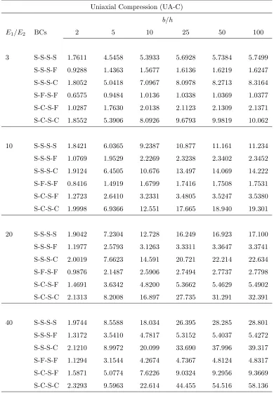
is given by the boundary condition S-C-S-C and the lowest by S-F-S-F. In Table 3 the results are given
for composite plates that are uniaxially loaded in the y direction, instead of the x direction for different
values of length-to-thickness and orthotropy ratios. The dimensionless critical buckling load is generally
lower for all the boundary conditions but for for the case with one or two sides free, namely, S-S-S-F and
S-F-S-F, it decreases significantly. The biaxial compression effect is examined and the results in Table
4 show as expected, a notable reduction in the critical buckling load, with respect to the uniaxial load
considered along x and y axes, respectively. In Table 5, results for moderately thick plate (a/h=10) with
the effect of the in-plane ratio (L/b) are presented for different values of orthotropy ratio. As can be seen
from this table, the critical buckling load decreases when increasing the in-plane ratio, independently for
all boundary conditions.
3.1. Buckling analysis of cross-ply composite stiffened plates
A particular feature of the DSM is that it allows the buckling analysis of stiffened plates in an exact
sense. Two different stiffened composite plate configurations shown in Fig. 5 and Fig. 6 respectively, are
analyzed and the results are discussed in this section. The geometrical parameters of the two stiffened
composite plates are given below:
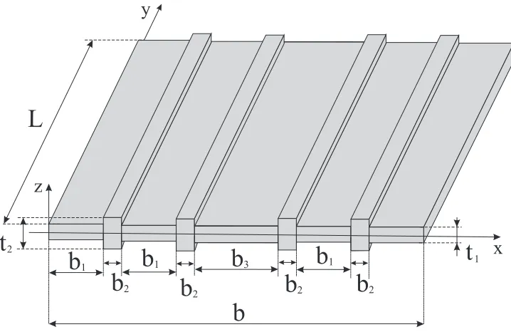
1. First stiffened composite plate configuration(Figure 5)
b= 1 m; L= 1 m; b1= 0.20 m; b2= 0.5 m; b3= 0.10 m; t1= 0.10 m; t2= 0.20 m;
2. Second stiffened composite plate configuration(Figure 6)
b= 1 m; L= 1 m; b1= 0.15 m; b2= 0.5 m; b3= 0.20 m; t1= 0.10 m; t2= 0.20 m;
In addition to the above stiffened panels, a simple uniform panel of thickness 0.002 m and with the same
of the dimensions has also been analyzed for comparative purposes. In Fig. 7 the dimensionless critical
buckling load for different boundary conditions are shown against the length-to-thickness ratio for the
two stiffened composite plates alongside the results of the simple panel of uniform thickness. The panels
were loaded in the x direction. As can be seen from the figure, the introduction of the stiffeners increases
the buckling loads very considerably, particularly for thin composite plates. On the contrary, when thick
composite plates are analyzed the increase is not so prominent. Clearly, the results are dependent on
the applied boundary conditions. Indeed, in the case of S-S-S-S boundary condition the use of stiffeners
increases the critical buckling load for both of the stiffened plate configurations. By contrast, using a
S-C-S-C boundary condition does not affect the critical buckling load so significantly. It is interesting to
note that the relative advantages of using the first or the second stiffened composite plate configurations
depend on the applied boundary conditions, although the differences in the dimensionless buckling loads
between the two configurations are sometimes rather small. In particular, when applying S-S,
S-S-S-C and S-S-S-C-S-S-S-C boundary conditions, the first stiffened composite plate configuration leads to higher
buckling load. Whilst, applying S-S-S-F, S-F-S-F and S-C-S-F the highest buckling loads are reached
corresponding to simple composite plates, first and second configurations of stiffened composite plates
are respectively shown. When presenting modes, square symmetric cross-ply plates made of five layers
and uniaxially loaded along the y direction are considered. It is now possible to provide an overview
of how the mode shapes change when changing the geometrical characteristics of the composite plate
assemblies. It should be noted that the mode shape of a S-S-S-S simple composite plate of uniform
thickness related to its critical buckling load is made up of two half-waves in the x direction and one
in the y direction. On the contrary, in either of the two stiffened composite plates the mode shape is
characterized by only one half-wave in both direction x and y. Other changes in the mode shapes related
to different boundary conditions can be observed in the same figures. The results are particularly useful
when controlling the mode shapes which generally have significant impact on response.
4. Concluding Remarks
An exact dynamic stiffness theory for composite plate elements using higher order shear deformation
theory is developed for the first time using the principle of minimum potential energy and symbolic
algebra to carry out buckling analysis in an exact sense. The theory is implemented in a computer
program to carry out buckling analysis of complex composite structures modelled as plate assemblies.
The proposed theory is a significant refinement over other dynamic stiffness theories using classical plate
theory and/or first order shear deformation theory. The developed DSM model is particularly useful
when analyzing thick composite plates with moderate to high orthotropic ratios for which the FEM
may become unreliable. A detailed parametric study has been carried out by varying significant plate
parameters and boundary conditions. The results have been critically examined and the theory has been
assessed using existing theories. Two different stepped composite plate configurations have been analyzed
for their stability behavior. Based on the computed results the following conclusions can be drawn:
• The exact HSDT plate element has been shown to be extremely accurate in terms of results and
computational efficiency when carrying out buckling analysis of composite plate assemblies.
• The exact HSDT plate element provides a significant refinement over to the FSDT element
partic-ularly when thick plate with a high orthotropy ratio are analyzed.
• The boundary conditions affect conspicuously the buckling modes.
• Stiffeners, if properly introduced increase the buckling load considerably.
• The buckling load of stiffened composite plates change prominently with respect to the simple
composite plate depending on the stiffeners position and on the applied boundary conditions.
5. Acknowledgement
References
[1] S. P. Timoshenko, Theory of elastic stability, McGraw Hill, New York, 1961.
[2] A. Leissa, Condition for laminated plates to remain flat under inplane loading., Composite Structures
6 (1986) 261–270.
[3] D. Bushnell, Computerized buckling analysis of shells, M. Nihhoff, Dordrecht, The Netherlands,
1985.
[4] E. Riks, Buckling, Encyclopedia of Computational Mechanics,edited by E. Stein, R. de Borst and
T.J.R. Hughes, Vol.2 Wiley, New York, 2004.
[5] F. A. Fazzolari, M. Boscolo, J. R. Banerjee, An exact dynamic stiffness element using a higher
order shear deformation theory for free vibration analysis of composite plate assemblies, Composite
Structures 96 (2013) 262–278.
[6] W. H. Wittrick, A Unified Approach to the Initial Buckling of Stiffened Panels in Compression,
Aeronautical Quarterly 19 (1968) 265–283.
[7] W. H. Wittrick, C. P. L. V., Stability Functions for the Local Buckling of Thin Flat-Walled Structures
with the Walls in Combined Shear and Compression, Aeronautical Quarterly 19 (1968) 327–351.
[8] W. H. Wittrick, General Sinusoidal Stiffness Matrices for Buckling and Vibration Analysis of Thin
Flat-Walled Structures, International Journal of Mechanical Sciences 10 (1968) 949–966.
[9] C. S. Smith, Bending, Bucking and Vibration of Orthotropic Plate-Beam Structures, Journal of Ship
Research 12 (1968) 249–268.
[10] F. W. Williams, Computation of Natural Frequencies and Initial Buckling Stresses of Prismatic
Plate Assemblies, Journal of Sound and Vibration 21 (1972) 87–106.
[11] W. H. Wittrick, F. W. Williams, Buckling and Vibration of Anisotropic or Isotropic Plate Assemblies
Under Combined Loadings, International Journal of Mechanical Sciences 16 (4) (1974) 209–239.
[12] R. Plank, W. H. Wittrick, Buckling Under Combined Loadings of Thin Flat-Walled Structures By a
Complex Finite-Strip Method, International Journal of Numerical Methods in Engineering 8 (1974)
323–339.
[13] W. H. Wittrick, F. W. Williams, An Algorithm for Computing Critical Buckling Loads of Elastic
Structures, Journal of Structural Mechanics 1 (3) (1973) 497–518.
[14] A. V. Viswanathan, M. Tamekuni, Elastic Buckling Analysis for Composite Stiffened Panels and
other Structures Subjected to Biaxial In-plane Loads, NASA Technical Report CR-2216.
[15] A. V. Viswanathan, M. Tamekuni, L. L. Tripp, Elastic Stability of Biaxially Loaded Longitudinally
Stiffened Composite Structures, Proceeding of the 14st AIAA/ASME/ASCE/AHS/ASC Structures,
[16] A. V. Viswanathan, M. Tamekuni, L. L. Baker, Elastic Stability of Laminated, Flat and Curved
Long Rectangular Plates Subjected to Combined Loads, NASA Technical Report CR-2330.
[17] F. W. Williams, M. S. Anderson, Incorporation of Lagrange Multipliers into an Algorithm for Finding
Exact Natural Frequencies or Critical Buckling Loads, International Journal of Mechanical Sciences
25 (8) (1983) 579–584.
[18] M. S. Anderson, F. W. Williams, C. J. Wright, Buckling and Vibration of any Prismatic Assembly
of Shear and Compression Loaded Anisotropic Plates with an Arbitrary Supporting Structures,
International Journal of Mechanical Sciences 25 (8) (1983) 585–596.
[19] M. S. Anderson, D. Kennedy, Inclusion of Transverse Shear Deformation in the Exact
Buckling and Vibration Analysis of Composite Plate Assemblies, Proceeding of the 32nd
AIAA/ASME/ASCE/AHS/ASC Structures, Structural Dynamics and Materials Conference,
Dal-las, Texas AIAA Paper 92-2287.
[20] J. R. Banerjee, Dynamic stiffness formulation for structural elements: A general approach,
Comput-ers & Structures 63 (1) (1997) 101–103.
[21] J. R. Banerjee, Free vibration analysis of a twisted beam using the dynamic stiffness method,
Inter-national Journal of Solids and Structures 38 (38-39) (2001) 6703–6722.
[22] J. R. Banerjee, Free vibration of sandwich beams using the dynamic stiffness method, Computers
and Structures 81 (18-19) (2003) 1915–1922.
[23] J. R. Banerjee, Development of an exact dynamic stiffness matrix for free vibration analysis of a
twisted timoshenko beam, Journal of Sound and Vibration 270 (1-2) (2004) 379–401.
[24] J. R. Banerjee, H. Su, D. R. Jackson, Free vibration of rotating tapered beams using the dynamic
stiffness method, Journal of Sound and Vibration 298 (4-5) (2006) 1034–1054.
[25] J. R. Banerjee, C. W. Cheung, R. Morishima, M. Perera, J. Njuguna, Free vibration of a
three-layered sandwich beam using the dynamic stiffness method and experiment, International Journal
of Solids and Structures 44 (22-23) (2007) 7543–7563.
[26] J. N. Reddy, A simple higher order theory for laminated plates., J. Appl. Mech. 51 (1984) 745–752.
[27] J. N. Reddy, D. Phan, Stability and vibration of isotropic , orthotropic and laminate plates according
to a higher-order shear deformation theory., Journal of Sound and Vibration 98 (2) (1985) 157–170.
[28] J. N. Reddy, T. Kuppusamy, Natural vibration of laminated anisotropic plates., Journal of Sound
and Vibration 94 (1) (1984) 63–69.
[29] B. Vlasov, On the equations of bending of plates, Dokla Ak Nauk Azerbeijanskoi SSR [in Russian]
3 (1957) 955–959.
[30] Jemielita, Technical theory of plates with moderate thickness., Rozprawy Inz [in Polish] 23 (1975)
[31] Jemielita, On kinematical assumptions of refined theories of plates., Journal of Applied Mechanics
57 (1990) 1088–1091.
[32] F. A. Fazzolari, E. Carrera, Advanced variable kinematics Ritz and Galerkin formulation for accurate
buckling and vibration analysis of laminated composite plates, Composite Structures 94 (1) (2011)
50–67.
[33] F. A. Fazzolari, E. Carrera, Accurate free vibration analysis of thermo-mechanically pre/post-buckled
anisotropic multilayered plates based on a refined hierarchical trigonometric Ritz formulation,
Com-posite Structures 95 (2013) 381–402.
[34] F. A. Fazzolari, E. Carrera, Advances in the Ritz formulation for free vibration
re-sponse of doubly-curved anisotropic laminated composite shallow and deep shells, Composite
Structures,doi:10.1016/j.compstruct.2013.01.018.
[35] F. A. Fazzolari, E. Carrera, Thermo-mechanical buckling analysis of anisotropic multilayered
com-posite and sandwich plates by using refined variable-kinematics theories, Journal of Thermal
Stresses,doi:10.1080/01495739.2013.770642.
[36] F. A. Fazzolari, E. Carrera, Free vibration analysis of sandwich plates with anisotropic face sheets
in thermal environment by using the hierarchical trigonometric Ritz formulation, Composites Part
B: Engineering,doi:10.1016/j.compositesb.2013.01.020.
[37] E. Carrera, F. A. Fazzolari, L. Demasi, Vibration analysis of anisotropic simply supported plates
by using variable kinematic and Rayleigh-Ritz method, Journal of Vibration and Acoustics 133 (6)
(2011) 061017–1/061017–16.
[38] F. A. Fazzolari, Fully coupled thermo-mechanical effect in free vibration analysis of anisotropic
multilayered plates by combining hierarchical plates models and a trigonometric Ritz formulation,
in: Mechanics of Nano, Micro and Macro Composite Structures Politecnico di Torino, 18-20 June,
2012.
[39] E. Carrera, On the use of transverse shear stress homogeneous and non-homogeneous conditions in
third-order orthotropic plate theory, Composite Structures 77 (2007) 341–352.
[40] J. N. Reddy, Mechanics of laminated composite plates and shells. Theory and Analysis, 2nd Edition,
CRC Press, 2004.
[41] Y. F. Xing, B. Liu, Exact solutions for the free in-plane vibrations of rectangular plates, International
Journal of Mechanical Sciences 51 (3) (2009) 246–255.
[42] C. I. Park, Frequency equation for the in-plane vibration of a clamped circular plate, Journal of
Sound and Vibration 313 (1-2) (2008) 325–333.
[43] D. Gorman, Exact solutions for the free in-plane vibration of rectangular plates with two opposite
[44] Y. F. Xing, B. Liu, New exact solutions for free vibrations of thin orthotropic rectangular plates,
Composite Structures 89 (4) (2009) 567–574.
[45] T. Kant, K. Swaminathan, Free Vibration of Isotropic, Orthotropic, and Multilayer Plates based on
Tables
Table 1: Dimensionless uniaxial buckling load (along x direction) Ncr = ¯Ncr b
2
E2h3, for simply supported cross-ply square
plates withb/h= 10,E1/E2= open,G12/E2=G13/E2= 0.6,G23/E2= 0.5,ν12=ν13= 0.25.
Stacking Sequence Models E1/E2
[0◦/90◦/90◦/0◦] 3 20 40
3D-Elasticity [45] 5.304 ∆†3D% 15.019 ∆3D% 22.881 ∆3D%
Classical L`evy’s solution HSDT 5.393 (1.68) 15.298 (1.86) 23.340 (2.01) FSDT 5.399 (1.79) 15.351 (2.21) 23.453 (2.50) CLPT 5.754 (8.48) 19.712 (31.2) 36.160 (58.0)
DSM HSDT 5.393 (1.68) 15.298 (1.86) 23.340 (2.01)
† ∆3D% = ˆ ω−ˆω3D
ˆ
Table 2: Dimensionless uniaxial buckling load (along x direction) Ncr = ¯Ncr b
2
E2h3, for simply supported cross-ply square
plates, stacking sequence [0◦/90◦/90◦/0◦] andE1/E2= open,G12/E2=G13/E2= 0.6,G23/E2= 0.5,ν12=ν13= 0.25.
Uniaxial Compression (UA-C)
b/h
E1/E2 BCs 2 5 10 25 50 100
3 S-S-S-S 1.9557 4.5458 5.3933 5.6928 5.7384 5.7499
S-S-S-F 1.5912 3.3640 4.3496 5.4623 6.2621 6.8168
S-S-S-C 1.9821 5.4309 7.1169 7.8176 7.9304 7.9592
S-F-S-F 1.5839 3.2200 4.1087 5.1745 6.0137 6.7261
S-C-S-F 1.5954 3.3805 4.3651 5.4686 6.2624 6.8599
S-C-S-C 2.0555 6.8502 10.273 12.012 12.314 12.392
10 S-S-S-S 2.2810 7.1554 9.9406 11.209 11.420 11.473
S-S-S-F 2.0267 5.1516 6.9540 8.6366 9.7745 10.536
S-S-S-C 2.3426 8.3895 14.133 17.865 18.587 18.778
S-F-S-F 2.0040 4.5982 6.0871 7.9721 9.8185 11.836
S-C-S-F 2.0746 7.1554 7.0981 9.0614 10.724 12.305
S-C-S-C 2.5134 9.9930 20.515 30.068 32.273 32.878
20 S-S-S-S 2.5689 9.4219 15.298 18.825 19.482 19.654
S-S-S-F 2.3144 6.7586 9.8649 12.398 14.130 15.513
S-S-S-C 2.6643 10.376 20.977 31.075 33.495 34.166
S-F-S-F 2.2874 5.8285 8.1129 10.893 13.785 17.359
S-C-S-F 2.4425 7.0390 10.416 13.613 16.334 19.282
S-C-S-C 2.9945 11.723 28.670 52.336 59.682 61.870
40 S-S-S-S 3.0749 11.997 23.340 33.131 35.347 35.953
S-S-S-F 2.6827 8.7789 14.723 19.374 22.292 24.982
S-S-S-C 3.1136 12.301 29.414 54.096 62.190 64.645
S-F-S-F 2.6558 7.5209 11.386 15.744 20.251 26.398
S-C-S-F 2.9731 9.4057 15.987 21.955 26.517 31.952
Table 3: Dimensionless uniaxial buckling load (along y direction) Ncr = ¯Ncr b
2
E2h3, for simply supported cross-ply square
plates, stacking sequence [0◦/90◦/90◦/0◦] andE1/E2= open,G12/E2=G13/E2= 0.6,G23/E2= 0.5,ν12=ν13= 0.25.
Uniaxial Compression (UA-C)
b/h
E1/E2 BCs 2 5 10 25 50 100
3 S-S-S-S 1.7611 4.5458 5.3933 5.6928 5.7384 5.7499
S-S-S-F 0.9288 1.4363 1.5677 1.6136 1.6219 1.6247
S-S-S-C 1.8052 5.0418 7.0967 8.0978 8.2713 8.3164
S-F-S-F 0.6575 0.9484 1.0136 1.0338 1.0369 1.0377
S-C-S-F 1.0287 1.7630 2.0138 2.1123 2.1309 2.1371
S-C-S-C 1.8552 5.3906 8.0926 9.6793 9.9819 10.062
10 S-S-S-S 1.8421 6.0365 9.2387 10.877 11.161 11.234
S-S-S-F 1.0769 1.9529 2.2269 2.3238 2.3402 2.3452
S-S-S-C 1.9124 6.4505 10.676 13.497 14.069 14.222
S-F-S-F 0.8416 1.4919 1.6799 1.7416 1.7508 1.7531
S-C-S-F 1.2723 2.6410 3.2331 3.4805 3.5247 3.5380
S-C-S-C 1.9998 6.9366 12.551 17.665 18.940 19.301
20 S-S-S-S 1.9042 7.2304 12.728 16.249 16.923 17.100
S-S-S-F 1.1977 2.5793 3.1263 3.3311 3.3647 3.3741
S-S-S-C 2.0019 7.6623 14.591 20.721 22.214 22.634
S-F-S-F 0.9876 2.1487 2.5906 2.7494 2.7737 2.7798
S-C-S-F 1.4691 3.6342 4.8200 5.3662 5.4629 5.4902
S-C-S-C 2.1313 8.2008 16.897 27.735 31.291 32.391
40 S-S-S-S 1.9744 8.5588 18.034 26.395 28.285 28.801
S-S-S-F 1.3172 3.5410 4.7817 5.3152 5.4037 5.4272
S-S-S-C 2.1210 8.9972 20.099 33.690 37.996 39.317
S-F-S-F 1.1294 3.1544 4.2674 4.7367 4.8124 4.8317
S-C-S-F 1.5871 5.0774 7.6226 9.0324 9.2956 9.3669
Table 4: Dimensionless biaxial buckling load Ncr = ¯Ncr b
2
E2h3, for simply supported cross-ply square plates, stacking
sequence [0◦/90◦/90◦/0◦] andE1/E2= open,G12/E2=G13/E2= 0.6,G23/E2= 0.5,ν12=ν13= 0.25.
Biaxial Compression (BA-C)
b/h
E1/E2 BCs 2 5 10 25 50 100
3 S-S-S-S 1.1023 2.2729 2.6967 2.8464 2.8692 2.8750
S-S-S-F 0.7380 1.1497 1.2769 1.3521 1.3852 1.4067
S-S-S-C 1.1933 2.9361 3.8771 4.2793 4.3446 4.3614
S-F-S-F 0.6667 0.9694 1.0398 1.0645 1.0700 1.0724
S-C-S-F 0.7982 1.3461 1.5636 1.7234 1.8048 1.8605
S-C-S-C 1.3088 3.8427 5.7863 6.8039 6.9824 7.0288
10 S-S-S-S 1.2983 3.5777 4.9703 5.6045 5.7098 5.7368
S-S-S-F 0.8614 1.5689 1.8270 1.9946 2.0841 2.1516
S-S-S-C 1.3940 4.4697 7.6189 9.7570 10.177 10.289
S-F-S-F 0.8433 3.5777 1.6939 1.7622 1.7749 1.7794
S-C-S-F 0.9938 2.0208 2.5026 2.9029 3.1589 3.3695
S-C-S-C 1.5359 5.4652 9.8391 13.602 14.490 14.737
20 S-S-S-S 1.4291 4.7109 7.6492 9.4124 9.7410 9.8271
S-S-S-F 0.9639 2.0760 2.5673 2.8809 3.0531 3.1949
S-S-S-C 1.5490 5.5364 11.204 18.325 16.920 18.717
S-F-S-F 0.9876 2.1483 2.5978 2.7668 2.7959 2.8048
S-C-S-F 1.1486 2.7954 3.7130 4.4580 4.9542 5.4076
S-C-S-C 1.7409 6.6190 15.867 29.452 33.783 35.082
40 S-S-S-S 1.5757 2.8554 11.670 16.566 17.673 17.976
S-S-S-F 1.0707 15.582 3.9151 4.5807 4.9204 5.2192
S-S-S-C 1.7588 6.7056 15.582 29.298 33.968 35.400
S-F-S-F 1.1290 4.7504 4.2561 4.7504 4.8338 4.8566
S-C-S-F 1.3103 3.9332 5.8466 7.3603 8.3119 9.2536
Table 5: Dimensionless uniaxial buckling load (along x direction) Ncr = ¯Ncr b
2
E2h3, for simply supported cross-ply square
plates, stacking sequence [0◦/90◦/90◦/0◦] andE1/E2 = open,G12/E2=G13/E2= 0.6,G23/E2= 0.5,ν12=ν13= 0.25 andb/h= 10.
Uniaxial Compression (UA-C)
BCs
E1/E2 L/b S-S-S-S S-S-S-F S-S-S-C S-F-S-F S-C-S-F S-C-S-C
3 0.5 18.183 12.767 19.233 12.776 12.794 21.724
1 5.3933 4.3495 7.1169 4.1087 4.3651 10.273
2 2.8193 0.9613 4.8157 1.4112 1.6563 8.1889
3 2.4587 0.4922 4.4819 0.8937 1.2931 7.8872
10 0.5 28.622 18.999 29.988 19.095 19.232 28.622
1 9.9406 6.9540 14.133 6.0871 7.0981 20.515
2 6.9366 1.3132 11.576 2.0381 3.3398 18.337
3 6.5724 0.7331 11.259 1.4060 2.9245 18.074
20 0.5 37.688 25.547 38.880 25.650 25.796 41.504
1 15.298 9.8649 20.977 8.1129 10.416 28.670
2 11.650 1.7286 17.929 2.6008 5.4332 26.143
3 11.270 0.9827 17.609 1.8724 4.9325 25.888
40 0.5 47.531 34.730 47.734 34.765 34.798 48.892
1 23.340 14.723 29.414 11.386 15.987 37.045
2 18.414 2.4441 25.291 3.4376 9.0464 33.705
Figures
FSDT
HSDT
x,y
x
z
[image:28.612.69.527.242.468.2]y
Figure 1: Kinematic descriptions of FSDT and HSDT for a multilayered plates.
1
2
N
x z
y
Global Dynamic Stiffness Matrix
Dynamic Stiffness Matrices
SSSS
SSSF
SSSC
y
x
y
y
x
x
SFSF
SCSF
SCSC
y
x
y
y
[image:29.612.72.524.59.656.2]x
x
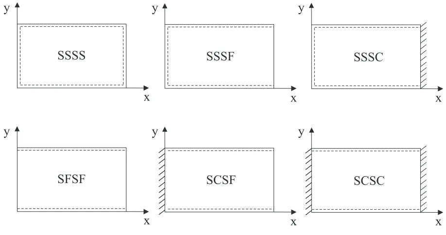
Figure 3: Boundary conditions.
y
x
N
y
0N
0N
0N
0x
L
b
[image:29.612.68.527.63.305.2]b
L
t
t
b
1b
1b
1b
b
11b
2b
3b
22 1
x
y
[image:30.612.118.474.79.266.2]z
Figure 5: 1st stiffened composite plate configuration.
[image:30.612.117.476.409.642.2]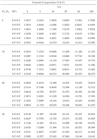

![Table 5: Dimensionless uniaxial buckling load (along x direction) Ncrandplates, stacking sequence [0 = N¯crb2E2 h3 , for simply supported cross-ply square◦/90◦/90◦/0◦] and E1/E2 = open, G12/E2 = G13/E2 = 0.6, G23/E2 = 0.5, ν12 = ν13 = 0.25 b/h = 10.](https://thumb-us.123doks.com/thumbv2/123dok_us/1539886.106546/27.612.95.502.185.613/dimensionless-uniaxial-buckling-direction-ncrandplates-stacking-sequence-supported.webp)

![Figure 7: Dimensionless uniaxial buckling loads NGcr = N¯crb2E2 h3 along the x direction varying the length-to-thicknessratio for simple and stiffened cross-ply plates, stacking sequence [0◦/90◦/0◦/90◦/0◦], step ratio t2/t1 = 2 and E1/E2 = 5,12/E2 = G13/E2 = 0.6, G23/E2 = 0.5, ν12 = ν13 = 0.25.](https://thumb-us.123doks.com/thumbv2/123dok_us/1539886.106546/31.612.76.515.49.661/dimensionless-uniaxial-buckling-direction-thicknessratio-stiened-stacking-sequence.webp)
![Figure 8: First buckling modes of simple cross-ply plates, lamination scheme [0◦/90◦/0◦/90◦/0◦] under uniaxial compressionalong the y direction, length-to-thickness ratio b/h=10 and orthotropic ratio E1/E2=25.](https://thumb-us.123doks.com/thumbv2/123dok_us/1539886.106546/32.612.81.517.45.665/figure-buckling-lamination-uniaxial-compressionalong-direction-thickness-orthotropic.webp)
![Figure 9:First buckling modes for the first stiffened cross-ply plate configurations Fig.[05, lamination scheme◦/90◦/0◦/90◦/0◦] under uniaxial compression along the y direction, length-to-thickness ratio b/h=10 and orthotropicratio E1/E2=25.](https://thumb-us.123doks.com/thumbv2/123dok_us/1539886.106546/33.612.87.512.49.672/stiened-congurations-lamination-uniaxial-compression-direction-thickness-orthotropicratio.webp)
