Time-domain analysis of substructure of a floating offshore wind turbine in waves

Proceedings of the ASME 2016 35th International Conference on Ocean, Offshore and Arctic Engineering OMAE2016 June 19-24, 2016, Busan, Korea

OMAE 2016-54113

TIME-DOMAIN ANALYSIS OF SUBSTRUCTURE OF A FLOATING OFFSHORE

WIND TURBINE IN WAVES

Zi Lin

State Key Laboratory of Ocean Engineering,Shanghai Jiaotong University,

Shanghai, China

Department of Naval Architecture, Ocean and Marine Engineering, University of Strathclyde

Glasgow, UK

Longbin Tao

School of Marine Science and Technology, University of Newcastle Upon Tyne

Newcastle, UK

P. Sayer

Department of Naval Architecture, Ocean and Marine Engineering, University of Strathclyde

Glasgow, UK

Dezhi Ning

State Key Laboratory of Coastal and Offshore Engineering, Dalian University of Technology

Dalian, China

ABSTRACT

This paper aims to analyze the dynamic response of a floating offshore wind turbine (FOWT) in waves. Instead of modeling the incident random wave by the traditional wave spectrum and superposition theory, an impulse response function method was used to simulate the incident wave. The incident wave kinematics were evaluated by a convolution of the wave elevation at the original point and the impulse response function in the domain. To check the validity of current wave simulation method, the calculated incident wave velocities were compared with analytical solutions; they showed good agreement. The developed method was then used for the hydrodynamic analysis of the substructure of the FOWT. A direct time-domain method was used to calculate the wave-rigid body interaction problem. The proposed numerical scheme offers an effective way of modeling the incident wave by an arbitrary time series.

INTRODUCTION

Offshore wind energy is a promising alternative energy source to traditional energy. Fixed offshore wind turbines are widely operated in shallow water depth while floating wind turbines become increasingly popular in deep water. Designing an offshore wind turbine requires a fully coupled integrated analysis, incorporating the aerodynamic analysis, structural analysis and hydrodynamic analysis arising from a combination

of environmental loadings. Wave loading, arising from the movement of seawater, is one of the most important aspects.

profile around the floating body were compared to check the validity of current numerical modeling.

NOMENCLATURE

ω

Circular frequency

w

Φ Incident potential

s

Φ Scattered potential

Φ

Velocity potential

i

_{Complex value}

ρ

Density of fluid

η

_{Wave elevation}

A Wave amplitude

B Damping matrix

BVP Boundary Value Problem

C Restoring matrix

F Wave force

FOWT Floating Offshore Wind Turbine g Acceleration due to gravity

G Green function

h Impulse response function

H Transfer function

HOBEM Higher order boundary element method

K Stiffness matrix

k Wave number

M Mass matrix

n Normal unit vector

p Wave pressure

r Radius between origin and calculated field r0 Radius between origin and inner damping layer r1 Radius between origin and outer damping layer

Sb Body surface

Sf Free surface

t Time

X Floating body motion response x,y and z Space coordinate

α Floating body angular motion response

α0, β0 and λ Damping coefficients

β Wave direction

ξ Floating body transverse motion response METHODOLOGY

Mathematical modeling for the incident wave

An impulse response function method was used to simulate the incident wave (King, 1986). Under linear system theory, the relationship between input x and output y for a system can be expressed as (Newland, 1978):

y(t)= h(t)x(t−τ)dτ −∞

∞

∫

(1) Similarly, for the problem of wave propagation, wave potential and its derivatives in the field can be written as:

Φ(t)= h(t)η(t-t)dt -∞

∞

∫

(2)

For linear wave theory, velocity potential and its derivatives have the following form:

Φ(x,y,z,t)=Re{igA ω e

kz_e−ik(xcosβ+ysinβ)_eiωt_}

(3) ( cos sin )

( , , , )

Re{ kz ik x y i t}

x y z t

gA e e t

β β ω

− +

∂Φ

= −

∂ (4)

and the corresponding wave profile η=Re{Aeiωt_}

(5) where Re denotes the real part. The following parts will describe how the analytical solution of h is calculated.

Considering a sinusoidal wave with an amplitude of A (eq.5), the corresponding velocity potential is shown in eq 3. So the transfer function can be written as

( cos sin )

( , , , )

kz ik x y

t

H

x y z

ge e

β β

ω

− +

∂Φ ∂

=

−

(6)

Using Inverse Fourier Transform, the analytical solution of the impulse response function was calculated from linear wave transfer function (eq 6). The analytical equation for impulse response function can be written as:

h_∂Φ

∂t

(t,x,y,z)

= H_∂Φ

∂t

(x,y,z)eiωt

−∞ ∞

∫

dω

=− g

2π e

kz_e−ik(xcosβ+ysinβ)_eiωt

−∞ ∞

∫

dω

(7)

The final analytical form of the impulse response function h was given by King (1986):

h_∂Φ ∂t

(t,x,y,z)

=−g

2π

πg

−z+i(xcosβ+ysinβ)w

t g

2 −z+i(xcosβ+ysinβ) ⎛ ⎝ ⎜ ⎜ ⎞ ⎠ ⎟ ⎟ (8)

The derivation of _h ∂Φ ∂x

and _h

∂Φ ∂z

is the same as _h ∂Φ ∂t

.

where w is the error function for complex values (Abramowitz and Stegun, 1964).

The incident wave kinematics and acceleration in the field were evaluated by a convolution of the wave elevation at the original point and the impulse response function in the domain (eq 2).

Mathematical and numerical modeling for wave-structure interaction problems

For wave-structure interaction problems, assuming non-viscous, non-rotational and incompressible flow, the velocity potential Φ satisfies the following equations in the fluid domain

∇2Φ=0 (9)

Unlike the indirect time-domain method (Cummins, 1962), the direct time-domain method deals with the diffracted and radiated wave (Isaacson and Cheung, 1992)

2 s₌₀

∇ Φ (11)

[image:3.612.73.272.125.434.2]

Figure 1 shows a sketch of calculation field and definition of coordinate. For linear wave-body interaction problems, the following boundary conditions have to be satisfied

Figure 1 Definition of sketch

Figure 2 Sketch of damping layer Free-surface condition

Using Taylor Series Expansion to first-order, the kinematic and dynamic conditions on the mean free surface can be written as (Ferrant, 1993):

s s ( ) z s _r t η ν η ∂ ∂Φ = −

∂ ∂ (12)

s ( ) t

s s

gη ν r

∂Φ

=− − Φ

∂ (13)

where

ν(r)= α0ω

r−r0

β0λ

⎛ ⎝ ⎜⎜ ⎞ ⎠ ⎟⎟ 0 ⎧ ⎨ ⎪ ⎩ ⎪ 2

r0≤r≤r1=r0+β0λ r<r0

Seabed condition

Assuming infinite water depth, velocity potential becomes zero with the increasing of water depth, so the following seabed condition has to be satisfied:

lim 0 z z→−∞ ∂Φ = ∂ (14)

Body surface condition

The kinematic condition on the mean wetted body surface can be expressed as

∂Φs

∂n =− ∂Φw

∂n +

(

ξ+α×X'

)

⋅n

(15) Radiation condition

An artificial damping layer has been added to avoid wave reflection, which has the same form as eqs 12 and 13. Figure 2 shows a sketch of damping layer.

The velocity potential in the field can be calculated by solving the following integral equation:

( 0) _{( )}

0 0

, ( )

( ) ( ) s ,

s s

s

G x x x

x x G x x ds

n n

αΦ = ⎡_⎢∂ Φ −∂Φ ⎤_⎥

∂ ∂

⎣ ⎦

∫∫ ₍₁₆₎

where α denotes the solid angle and the Green function has the following form

G x

(

,x0

)

=− 1 4π

1

x−xo

(

)

2+

(

y−yo

)

2

+

(

z−zo

)

2

A higher-order boundary element method (Bai and Teng, 2001) was applied for solving the integral equation numerically:

=1

( , ) K k( , ) k k

h

ξ ς ξ ς

Φ =

_∑

Φ

(17)

1

( , ) K _{( , )} k k

k h

n n

ξ ς _{ξ ς}

=

∂Φ ₌ ⎛∂Φ⎞ ⎜ ⎟

∂ ∑ ⎝∂ ⎠ (18)

Motion equation of the floating body was solved in the time domain directly:

Mi

⎡

⎣ ⎤⎦X

••

i(t)+⎡⎣Bi⎤⎦X •

i(t)+⎡_⎣K_i+C_i⎤_⎦Xi(t)

⎧ ⎨ ⎩ ⎫ ⎬ ⎭ i=1 6

∑ =Fi(t)

(19) Velocity potential and wave profile were updated by a 4th_{-order Runge-Kutta method. Only first-order forces were}

considered in current study. Wave forces acting on a floating body was evaluated by Bernoulli equation:

p=−ρ(∂Φ

∂t+

1

2∇Φ⋅ ∇Φ+gz)

(20)

VALIDATION OF THE IMPULSE RESPONSE

FUNCTION METHOD

For validation purpose, a surface-piercing cylinder with 1m- draft and 1m- radius was selected (vertical center of gravity=-0.6). For validation purpose, here we choose the wave circular frequency=0.6 rad/s and wave amplitude=1m. To prevent the cylinder from drift away, an artificial stiffness matrix (109 _{kN/m) was added into motion equation during}

simulation. Figures 3.1-2.3 show a comparison of incident wave potential between present impulse response method and analytical solution. Figures 4.1-4.3 describe a comparison of wave forces. From the comparison we can see that very good agreement has been found between the two methods, offering a good preparation for the following case studies.

[image:4.612.63.243.61.572.2] [image:4.612.347.524.85.222.2]

Figure 3.1 Comparison of velocityΦ_t

Figure 3.2 Comparison of velocityΦx

Figure 3.3 Comparison of velocityΦz

Figure 4.1 Comparison of wave forces, surge

Figure 4.2 Comparison of wave forces, heave

Figure 4.3 Comparison of wave forces, pitch CASE STUDIES

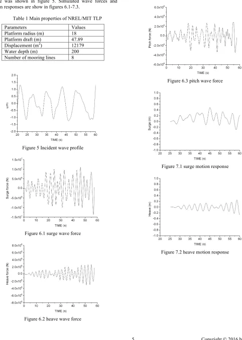
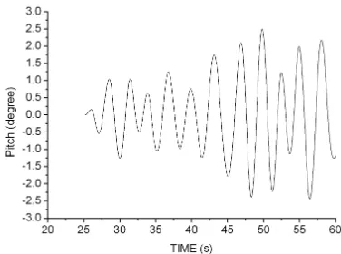
[image:4.612.349.525.252.394.2] [image:4.612.349.525.423.564.2]

profile was shown in figure 5. Simulated wave forces and motion responses are show in figures 6.1-7.3.

Table 1 Main properties of NREL/MIT TLP

Parameters Values

Platform radius (m) 18 Platform draft (m) 47.89 Displacement (m2_{) 12179}

Water depth (m) 200

[image:5.612.59.541.76.752.2]

Number of mooring lines 8

Figure 5 Incident wave profile

Figure 6.1 surge wave force

Figure 6.2 heave wave force

[image:5.612.352.543.83.406.2]

Figure 6.3 pitch wave force

[image:5.612.67.308.99.713.2]

Figure 7.1 surge motion response

[image:5.612.357.541.431.568.2]

[image:6.612.68.256.84.224.2]

Figure 7.3 pitch motion response

CONCLUSIONS AND FURTHER STUDIES

A direct time-domain numerical code has been developed and its accuracy has been validated by a comparison between present results and analytical solutions. The developed numerical method represents an advance in simulating an incident wave by an arbitrary time history. This is an on-going research. Further study will include dynamic modeling of mooring line responses and aerodynamic loadings. Further validation of present method will be carried out by a comparison between numerical and experimental results. Guidance will be discussed about the suitability of different methods of analysis and advantages of different types of floating structures.

REFERENCES

1. Roald, L., Jonkman, J.,Robertson, A.,Chokani,N.,2013.The effect of second-order hydrodynamics on floating offshore wind turbines. Energy Procedia, 35, pp. 253-264.

2. Karimirad, M., 2013.Modeling aspects of a floating wind turbine for coupled wave-wind-induced dynamic analyses. Renewable Energy, 53, pp. 299-305.

3. Newland D. E. 1987, An Introduction to Random Vibrations and Spectral Analysis, Longman, London, in Chinese by the National Publishing Corporation, Peking. 4. Bradley K.K., 1987, Time-domain analysis of wave

exciting forces on ships and bodies. Ann Arbor: The University of Michigan, Appendix A.

5. Abramowitz and Stegun., 1964, Handbook of Mathematical Functions. Courier Corporation.

6. Cummins W.E., 1962, The impulse response function and ship motions, DTMB Report 1661, Washington D.C. 7. Isaacson M. and Cheung K.F., 1992, Time-domain

second-order wave diffraction in three dimension. J Waterway, Port, Coastal and Ocean Eng., ASCE, 118(5), 496~516.

8. Bai W. and Teng B., 2001, Second-order wave diffraction around 3-D bodies by a time-domain method, China Ocean Eng, 15(1), 73-85.

9. Ferrant P. ,1993, Three-dimensional unsteady wave-body interactions by a Rankine boundary element method. Ship Technology Research, 165-175.