A stochastic differential equation model for the spread of HIV amongst people who inject drugs

(1)

Research Article

A Stochastic Differential Equation Model for the Spread

of HIV amongst People Who Inject Drugs

Yanfeng Liang, David Greenhalgh, and Xuerong Mao

Department of Mathematics and Statistics, University of Strathclyde, Glasgow G1 1XH, UK Correspondence should be addressed to Yanfeng Liang; yanfeng.liang@strath.ac.uk

Received 8 October 2015; Revised 7 December 2015; Accepted 22 December 2015

Academic Editor: Chuangyin Dang

Copyright © 2016 Yanfeng Liang et al. This is an open access article distributed under the Creative Commons Attribution License, which permits unrestricted use, distribution, and reproduction in any medium, provided the original work is properly cited.

We introduce stochasticity into the deterministic differential equation model for the spread of HIV amongst people who inject drugs (PWIDs) studied by Greenhalgh and Hay (1997). This was based on the original model constructed by Kaplan (1989) which analyses the behaviour of HIV/AIDS amongst a population of PWIDs. We derive a stochastic differential equation (SDE) for the fraction of PWIDs who are infected with HIV at time. The stochasticity is introduced using the well-known standard technique of parameter perturbation. We first prove that the resulting SDE for the fraction of infected PWIDs has a unique solution in (0, 1) provided that some infected PWIDs are initially present and next construct the conditions required for extinction and persistence. Furthermore, we show that there exists a stationary distribution for the persistence case. Simulations using realistic parameter values are then constructed to illustrate and support our theoretical results. Our results provide new insight into the spread of HIV amongst PWIDs. The results show that the introduction of stochastic noise into a model for the spread of HIV amongst PWIDs can cause the disease to die out in scenarios where deterministic models predict disease persistence.

1. Introduction

HIV (human immunodeficiency virus) is a deadly and infectiousLentiviruswhich attacks and weakens the immune system by especially attacking the CD4 cells. As a result, HIV causes AIDS (acquired immune seficiency syndrome). Since the first discovery of HIV in 1981, it has already infected almost 78 million people with about 39 million lives having been taken [1]. Despite the massive improvement in technology and medical equipment, we are still unable to fully find a cure for the HIV virus. In 2014, according to the reports by the World Health Organization, there were still approximately 36.9 million people living with HIV, with around 2 million new cases globally [2]. In order to control the epidemic, it is crucial to understand the dynamical behaviour of HIV and how it spreads within our community. There are various routes by which HIV can be transmitted, for example, transmission via unprotected sexual intercourse, vertically from infected mothers to their unborn children and people who inject drugs (PWIDs) sharing contaminated needles. Amongst all the possible routes of HIV transmission, PWIDs have become a significant risk group with around 3

million of them living with HIV [3]. For every 10 new cases of HIV infection, on average, one of them is caused by injecting drug use. In regions of Central Asia and Eastern Europe, injecting drug use accounts for 80 percent of HIV infections [3]. As a result, in this paper, we will focus on looking at this particular risk group.

Over the past years, mathematical models have been used successfully to analyse and predict the dynamical behaviour in biological systems. The first mathematical model for the spread of HIV and AIDS amongst PWIDs in shooting galleries was created by Kaplan [4], where a shooting gallery is a place for PWIDs to purchase and inject drugs. Kaplan incor-porated many factors into his model such as the injection equipment sharing rate and the effect of cleaning injection equipment in order to better understand how HIV is trans-mitted within this type of community. Based on the original model created in [4], Greenhalgh and Hay [5] modified the model by changing some of the assumptions made by Kaplan to make them more realistic. These assumptions include having different visiting rates to the shooting galleries for PWIDs who have been diagnosed positive for the HIV virus and thus may have been advised to stop sharing injections

(2)

and for those who either are not HIV positive or are but do not know it. The modified Kaplan model in [5] also allows for the possibility that an infected PWID may not always leave a needle infected before cleaning, as well as introducing different transmission probabilities for flushed and unflushed needles. The term “flushing” refers to the process where an infectious piece of injecting equipment is used by an uninfected PWID and thus after injecting the syringe is left uninfected. The HIV model that we will be looking at in this paper is based on the modified Kaplan model given in [5]. There have been many papers that have already looked at the connection between the spread of HIV and PWIDs [6–11]. However the models used are all deterministic models.

The real world is not deterministic, and there are many factors that can influence the behaviour of a disease and thus it is not always possible to predict with certainty what would happen. Consequently, a stochastic model would be more appropriate. Furthermore, a stochastic model also possesses many useful unique properties such as being able to calculate the probability that an endemic will not occur and the expected duration of an endemic. By running a stochastic model many times, we can also build up a distribution of the possible outcomes which allows us to identify the number of infectives at a particular time 𝑡, whereas for a deterministic model we will only get a single outcome. HIV infection is a behavioural disease and thus there are many environmental factors that can influence the spread of HIV. Rhodes et al. [12] have mentioned in detail how factors such as injecting environments, social network, and neighbourhood deprivation and poverty can affect the spread of HIV amongst PWIDs. There are also other papers which emphasised how the dynamical behaviour of HIV is highly correlated with other factors [13–15]. Consequently, it is crucial for us to understand how HIV would spread under those environ-mental influences, especially amongst PWIDs. In this case, a stochastic model would be useful. There is also natural biological variation within people in their response to HIV. Using a stochastic model with environmental perturbation in the disease transmission parameter as we will do is one way to include this.

The stochastic aspects of the HIV model have been studied by many authors. For example, in [16], Dalal et al. considered a stochastic model for internal HIV dynamics. They incorporated environmental stochasticity into their model by using the standard technique of parameter per-turbation. They proved that the solution (representing the concentrations of uninfected cells, infected cells, and virus particles) is nonnegative and have looked at the stability aspect of their model by establishing the conditions required in order for the numbers of infected cells and virus particles to tend asymptotically to zero exponentially almost surely. Ding et al. [13] looked at a stochastic model for AIDS transmission and control taking into consideration the treatment rate of HIV patients. They have also examined the effect that knowledge, attitude, and behaviour of patients have on the spread of AIDS. Tuckwell and Le Corfec [17] used a stochastic model to analyse the behaviour of HIV-1 but focus only on the early stage after infection. Dalal et al. [18] have also used a stochastic model to look at another aspect of HIV. Once again,

by using parameter perturbation, they introduced environ-mental randomness into their HIV model which allows them to examine the effect that condom use has on the spread of AIDS among a homogeneous homosexual population which is split into distinct risk groups according to the tendency of individuals to use condoms. Peterson et al. [19] constructed a population-based simulation of a community of PWIDs using the Monte Carlo technique. Greenhalgh and Lewis [20] modelled the spread of disease using a set of behavioural assumptions due to Kaplan and O’Keefe [10]. They use a branching process approximation to show that if the basic reproduction number𝑅₀is less than or equal to unity then the disease will always go extinct. They calculate an expression for the probability of extinction. They discuss an extended model which incorporates a three-stage incubation period and again examine a branching process approximation. They then compare them to investigate whether the deterministic model provides a good approximation to the simulated stochastic model. Although there have been many papers that looked at the stochastic aspect of the spread of HIV, as far as we know there are not many studies that focus on the stochastic aspect of the spread of HIV amongst PWIDs despite this particular risk group being responsible for many new HIV cases around the world. Thus it is crucial for us to examine the effect of environmental noise on this type of community.

Inspired by the model constructed in [5], in this paper we will introduce environmental stochasticity into the model by parameter perturbation which is a standard technique in stochastic population modelling [16, 18, 21, 22]. To the best of our knowledge, this is the first paper which examines the effect that environmental stochasticity has on the dynamical behaviour of the modified Kaplan model [5]. The techniques used in this paper are inspired by the work done in [21]. The paper is organised as follows. In the next section, we will describe the formulation of the stochastic HIV model amongst PWIDs. In Section 3, we shall prove the existence of a unique nonnegative solution. In Sections 4 and 5, we will investigate two of the main important properties of any biological system, namely, the conditions required for extinction and persistence, respectively. Then in Section 6, we shall show that there exists a stationary distribution for our system. Finally, we will perform some numerical simulations with realistic parameter values to verify the results.

2. The Stochastic HIV Model

Throughout this paper, we let (Ω, F, {F_𝑡}_𝑡≥0, P) be a complete probability space with filtration{F_𝑡}_𝑡≥0 satisfying the usual conditions (i.e., it is increasing and right continuous whileF₀contains allP-null sets). Let us consider the follow-ing deterministic HIV model, which has been constructed by Greenhalgh and Hay [5] based on the model of Kaplan [4]. Define the following parameters:

(3)

𝜆₂: shooting gallery visiting rate for infected PWIDs who know that they are infected.

𝑃₁: probability that the needle is flushed and the PWID is infected.

𝑃₂: probability that the needle is flushed and the PWID remains uninfected.

𝑃3: probability that the PWID becomes infected

without the needle being flushed.

𝑃₄: probability that the PWID remains uninfected and the needle is not flushed.

𝜙₁: probability that an infected PWID leaves unin-fected a syringe that was initially uninunin-fected.

𝜃₁: probability that an infected PWID leaves unin-fected a syringe that was initially inunin-fected.

𝜉: fraction of all PWIDs (susceptible or not) who bleach their injection equipment after use.

𝛾: gallery ratio, where𝛾 = 𝑛/𝑚and𝑛represents the PWID population and𝑚represents the number of shooting galleries or syringes that each PWID visits at random.

𝑝: probability that infected PWIDs know that they are infected.

𝜇: per capita rate at which infected PWIDs cease to share injection equipment (including those who cease sharing because of developing AIDS).

Note that𝑃₁+ 𝑃₂+ 𝑃₃+ 𝑃₄= 1.

Define the following new composite parameters:

𝜎 = [𝜆₁(1 − 𝑝) + 𝜆₂𝑝] 𝛾 (1 − 𝜉) (1 − 𝜙1) ,

𝜂 = [𝜆₁(1 − 𝑝) + 𝜆₂𝑝] 𝛾 [𝜉 + 𝜃₁(1 − 𝜉)] , 𝜌 = 𝜆₁𝛾 [1 − (1 − 𝜉) (1 − 𝑃1− 𝑃2)] ,

𝜐 = 𝜆₁(𝑃₁+ 𝑃₃) .

(1)

In the expression for𝜎the factor(1−𝜉)(1−𝜙₁)represents the probability that an initially uninfected syringe is left infected and not cleaned by an infected PWID. The term𝜆₁(1 − 𝑝) +

𝜆₂𝑝represents the average rate at which an infected PWID visits syringes. Hence𝜎 = 𝛾𝜎, where𝛾 = 𝑛/𝑚is the gallery ratio and 𝜎 is the rate at which an infected PWID visits syringes multiplied by the probability that he or she leaves an uninfected syringe infected after use. Similarly𝜂 = 𝛾𝜂, where𝜂is the rate at which an infected PWID visits syringes multiplied by the probability that he or she leaves an infected syringe uninfected after use.

𝜆₁represents the rate at which a susceptible PWID visits syringes and1 − (1 − 𝜉)(1 − 𝑃₁− 𝑃₂)represents the probability that an initially infected syringe is left uninfected after use by that PWID. Hence𝜌 = 𝛾𝜌, where𝜌is the rate at which a susceptible PWID visits syringes multiplied by the probability that he or she leaves an infected syringe uninfected after use.𝜐represents the rate at which a susceptible PWID visits syringes multiplied by the probability that he or she becomes infected given that the syringe which they visit is infected.

Thus𝜐𝛽represents the rate at which a susceptible PWID visits syringes and becomes infected.𝜐can thus be regarded as the “potential” infection rate of a susceptible PWID.

Let 𝜋(𝑡) and 𝛽(𝑡) denote the proportion of infected PWIDs and proportion of infected needles, respectively. Thus the absolute numbers of infected PWIDs and infected needles are 𝑛𝜋(𝑡) and 𝑚𝛽(𝑡). The spread of the disease amongst syringes can be described by the following differential equa-tion:

𝑑 (𝑚𝛽 (𝑡))

𝑑𝑡 = 𝑛𝜋 (𝑡) 𝜎 (1 − 𝛽 (𝑡)) − 𝑛𝜋 (𝑡) 𝜂𝛽 (𝑡) − 𝑛 (1 − 𝜋 (𝑡)) 𝜌𝛽 (𝑡) .

(2)

Dividing by𝑚,

𝑑𝛽 (𝑡)

𝑑𝑡 = 𝜋 (𝑡) 𝜎 (1 − 𝛽 (𝑡)) − 𝜋 (𝑡) 𝜂𝛽 (𝑡) − (1 − 𝜋 (𝑡)) 𝜌𝛽 (𝑡)

= 𝜋 (𝑡) (𝜎 − 𝜏𝛽 (𝑡)) − (1 − 𝜋 (𝑡)) 𝜌𝛽 (𝑡) ,

(3)

where

𝜏 = 𝜎 + 𝜂 = 𝛾 (𝜎 + 𝜂) , (4)

is the gallery ratio multiplied by the rate at which an infected PWID visits syringes multiplied by the sum of the probability that he or she leaves an uninfected syringe infected after use plus the probability that he or she leaves an infected syringe uninfected after use.

The spread of the disease amongst PWIDs can be described by the differential equation:

𝑑 (𝑛𝜋 (𝑡))

𝑑𝑡 = 𝑛 (1 − 𝜋 (𝑡)) 𝜐𝛽 (𝑡) − 𝜇 (𝑛𝜋 (𝑡)) . (5)

Dividing by𝑛,

𝑑𝜋 (𝑡)

𝑑𝑡 = (1 − 𝜋 (𝑡)) 𝜐𝛽 (𝑡) − 𝜇𝜋 (𝑡) . (6)

So in summary the equations describing the deterministic HIV model are

𝑑𝛽 (𝑡)

𝑑𝑡 = 𝜋 (𝑡) (𝜎 − 𝜏𝛽 (𝑡)) − (1 − 𝜋 (𝑡)) 𝜌𝛽 (𝑡) , 𝑑𝜋 (𝑡)

𝑑𝑡 = (1 − 𝜋 (𝑡)) 𝜐𝛽 (𝑡) − 𝜇𝜋 (𝑡) .

(7)

Greenhalgh and Hay define the basic reproduction num-ber for the modified Kaplan model to be

𝑅𝐷₀ = 𝜐𝜎

𝜌𝜇, (8)

(4)

with the original infected PWID) caused during his or her entire infectious period by a single newly infected PWID entering a disease-free population at equilibrium. They also point out that it is also the expected number of secondary infected needles caused by a single newly infected needle entering the disease-free population at equilibrium.

Greenhalgh and Hay then show that the disease dies out if𝑅𝐷₀ < 1or𝑅𝐷₀ = 1and𝜏 > 𝜌. If𝑅𝐷₀ > 1 there are two possible equilibria, one with no disease present and the other with disease present. Thus this value of𝑅𝐷₀ clearly satisfies the usual properties of the deterministic threshold value in epidemic models. There is a unique endemic equilibrium

𝛽∗= 𝜎_𝜏(1 −𝜌𝜇_𝜎𝜐) ,

𝜋∗= 𝜎𝜐 − 𝜌𝜇 𝜇𝜏 + 𝜎𝜐 − 𝜌𝜇.

(9)

If𝑅𝐷₀ > 1 then the unique endemic equilibrium is locally stable. If𝜏 > 𝜌and𝑅𝐷₀ > 1, then𝛽(𝑡) → 𝛽∗and𝜋(𝑡) → 𝜋∗ as𝑡 → ∞provided that𝜋(0) > 0or𝛽(0) > 0.

Note that the average rate at which PWIDs leave the sharing, injecting population is around 0.25/year [5] so, on average, they each share for four years.𝑃₁+𝑃₃, the probability of HIV transmission to a susceptible PWID on making a single injection with an infected syringe, is quite small (e.g., one estimate is 0.01 [5]). On the other hand, PWIDs are injected every few days which is a much shorter timescale than the demographic epidemiological changes which take several years. Hence changes in the fraction of syringes infected will typically happen a lot faster than changes in the fraction of PWIDs infected.

Thus over an intermediate timescale it may be reasonable to assume that 𝜋(𝑡) is approximately constant in the last equation of (7). Hence 𝛽(𝑡) will approach its equilibrium value from this equation

𝜋 (𝑡) 𝜎

𝜋 (𝑡) + 𝜌 − 𝜌𝜋 (𝑡). (10)

By substituting (10) into the second equation in (7) we deduce that

𝑑𝜋 (𝑡)

𝑑𝑡 = (𝜋 (𝑡) 𝜏 + 𝜌 − 𝜋 (𝑡) 𝜌1 − 𝜋 (𝑡)) 𝜋 (𝑡) 𝜐𝜎 − 𝜇𝜋 (𝑡) . (11)

A similar technique of reducing the dimensions of the model by assuming that the needle equations are at equilibrium is used in models of variable infectivity of spread of HIV amongst PWIDs discussed by Greenhalgh and Lewis [8, 11] and Corson et al. [23, 24].

In this paper, we introduce environmental stochastic-ity into system (11) by replacing the parameter 𝜐 by 𝜐 +

𝜐(𝑑𝐵(𝑡)/𝑑𝑡), where𝐵(𝑡)is a Brownian motion and𝜐 > 0is the intensity of the noise which is associated with the potential rate of infection𝜐. It is therefore clear that the total number of new PWIDs infected during the small time interval[𝑡, 𝑡 + 𝑑𝑡) is normally distributed with mean,

𝑛 (1 − 𝜋 (𝑡)) 𝜋 (𝑡) 𝜐𝜎

𝜋 (𝑡) 𝜏 + 𝜌 − 𝜋 (𝑡) 𝜌𝑑𝑡, (12)

and variance,

𝑛2(1 − 𝜋 (𝑡))2𝜋 (𝑡)2𝜐2𝜎2

(𝜋 (𝑡) 𝜏 + 𝜌 − 𝜋 (𝑡) 𝜌)2 𝑑𝑡. (13)

Notice that both of this mean and variance tend to zero as𝑑𝑡goes to zero which is a biologically desirable property. This is a standard technique of introducing random noise in stochastic modelling [16, 18, 25–28] and corresponds to some stochastic environmental factor acting on each individual in the population.

To justify why simple white noise is appropriate for our model suppose that we consider a timescale on which𝛽(𝑡) and𝜋(𝑡)are approximately constant. We consider the changes in a small time interval[𝑡, 𝑡 + 𝑇₀)and divide it into a series of

𝑛₀equal width subintervals[𝑡, 𝑡 + 𝑇 ), [𝑡 + 𝑇, 𝑡 + 2𝑇 ), . . . , [𝑡 +

(𝑛₀ − 1)𝑇 , 𝑡 + 𝑛₀𝑇), where𝑛₀𝑇 = 𝑇₀ and𝑛₀ is very large. Then the numbers of new infections caused by a single susceptible PWID visiting one infected syringe during each of the subintervals[𝑡, 𝑡 + 𝑇 ), [𝑡 + 𝑇, 𝑡 + 2𝑇 ), . . . , [𝑡 + (𝑛₀ −

1)𝑇, 𝑡 + 𝑛₀𝑇) are identically distributed random variables, say, with common mean𝜇₀ and common variance 𝜎₀2. We assume that 𝜎₀2 < ∞. So by the Central Limit Theorem the total number of PWIDs who visit infected syringes and become infected in[𝑡, 𝑡 + 𝑛₀𝑇 ) = [𝑡, 𝑡 + 𝑇₀)is approximately normally distributed with mean 𝑛₀𝜇₀ and variance 𝑛₀𝜎₀2. Moreover keeping𝑇fixed and doubling𝑇₀ doubles𝑛₀thus the mean and variance of the number of susceptible PWIDs who become infected from visiting an infected syringe in

[𝑡, 𝑡 + 𝑇₀)are both proportional to𝑇₀. Hence it is appropriate to consider simple white noise where the mean number of infections in[𝑡, 𝑡 + 𝑑𝑡)caused by a given susceptible PWID visiting a given infected syringe is𝜐𝑑𝑡(hence proportional to

𝑑𝑡) the same as in the deterministic model and the variance of this number is also proportional to𝑑𝑡.

As a result, we obtain the following SDE HIV model:

𝑑𝜋 (𝑡) = [ (_{𝜋 (𝑡) 𝜏 + 𝜌 − 𝜋 (𝑡) 𝜌}1 − 𝜋 (𝑡)) 𝜋 (𝑡) 𝜐𝜎 − 𝜇𝜋 (𝑡)] 𝑑𝑡

+ [ (1 − 𝜋 (𝑡)) 𝜋 (𝑡) 𝜐𝜎

𝜋 (𝑡) 𝜏 + 𝜌 − 𝜋 (𝑡) 𝜌] 𝑑𝐵 (𝑡) .

(14)

The reason why we chose to perturb the parameter 𝜐 corresponding to the total rate at which PWIDs visit syringes and potentially become infected is because as it multiplies the term𝜋(1−𝜋)in (11) it is a key parameter in the transmission of HIV amongst PWIDs and we thought that this would be the most interesting and important parameter when analysing the effect that environmental noise would have on the spread of HIV.

(5)

insight into the behaviour of the model. A similar approach of introducing environmental stochasticity into only the disease transmission parameter was discussed in stochastic studies of epidemic models by Ding et al. [13], Gray et al. [21], Lu [25], Tornatore et al. [29], and others.

For the rest of the paper, we shall focus on analysing the SDE HIV model (14). Throughout this paper, unless stated otherwise, we shall assume that the unit of time is one day.

3. Existence of Unique Nonnegative Solution

Before we begin to investigate the dynamical behaviour of the SDE HIV model (14), it is important for us to show whether this SDE has a unique global nonnegative solution. It is well-known that, in order for an SDE to have a unique global solution for any given initial value, the coefficients of the equation are generally required to satisfy the linear growth condition and the local Lipschitz conditions [30]. It is clear that our coefficients in (14) satisfy the linear growth condition and they are locally Lipschitz continuous. As a result there is a unique, nonexplosive solution to (14). The following theorem shows that the solution remains in(0, 1)if it starts there.

Theorem 1. For any given initial value𝜋(0) = 𝜋₀∈ (0, 1), the SDE HIV model (14) has a unique global nonnegative solution

𝜋(𝑡) ∈ (0, 1)for all𝑡 ≥ 0with probability one; namely,

P{𝜋 (𝑡) ∈ (0, 1) , ∀𝑡 ≥ 0} = 1. (15)

Proof. For any given initial value𝜋₀∈ (0, 1), there is a unique global solution𝜋(𝑡)for𝑡 ≥ 0. Let𝑘₀ ≥ 0be sufficiently large so that𝜋₀lies within the interval(1/𝑘₀, 1 − (1/𝑘₀)). Then for each integer𝑘 ≥ 𝑘₀, define the stopping time

𝜏_𝑘=inf{𝑡 ≥ 0 : 𝜋 (𝑡) ∉ (1

𝑘, 1 − ( 1

𝑘))} , (16)

where inf0 = ∞. It is easy to see that𝜏_𝑘is increasing as𝑘 →

∞. Let us also define𝜏_∞=lim_𝑘→∞𝜏_𝑘. To complete the proof, we need to show that𝜏_∞= ∞a.s. We will carry this proof out by contradiction. Let us therefore assume that the statement is false and thus there exists a pair of constants𝑇 > 0and

𝜀 ∈ (0, 1)such that

P{𝜏_∞≤ 𝑇 } > 𝜀. (17)

Hence, there is an integer𝑘₁≥ 𝑘₀such that

P{𝜏_𝑘 ≤ 𝑇} > 𝜀 ∀𝑘 ≥ 𝑘₁. (18)

Let us define a function𝑉 : (0, 1) →R,

𝑉 (𝑥) = 1_𝑥+ 1

1 − 𝑥. (19)

Now by Itˆo’s formula, we have that, for any𝑡 ∈ [0, 𝑇 ]and

𝑘 ≥ 𝑘₁,

E𝑉 (𝜋 (𝑡 ∧ 𝜏_𝑘)) = 𝑉 (𝜋₀) +E∫𝑡∧𝜏𝑘

0 𝐿𝑉 (𝜋 (𝑠)) 𝑑𝑠, (20)

where𝐿𝑉 : (0, 1) →Ris defined by

𝐿𝑉 (𝑥) = _{𝑥 (𝑥𝜏 + 𝜌 − 𝑥𝜌)}− (1 − 𝑥) 𝜐𝜎 + 𝑥𝜐𝜎

(𝑥𝜏 + 𝜌 − 𝑥𝜌) (1 − 𝑥)

+𝜇 𝑥−

𝜇𝑥

(1 − 𝑥)2 + (1 − 𝑥)

2_𝜐2_𝜎2

(𝑥𝜏 + 𝜌 − 𝑥𝜌)2𝑥

+ 𝑥2𝜐2𝜎2 (1 − 𝑥) (𝑥𝜏 + 𝜌 − 𝑥𝜌)2.

(21)

Furthermore, it is easy to see that

𝐿𝑉 (𝑥) ≤ 𝜐𝜎

min(𝜏, 𝜌) (1 − 𝑥) +

𝜇 𝑥

+ 𝜐2𝜎2

min(𝜏, 𝜌)2[

1 𝑥 +

1

1 − 𝑥] ≤ 𝐶𝑉 (𝑥) ,

(22)

where

𝐶 = {[ 𝜐𝜎

min(𝜏, 𝜌)] ∨ 𝜇} +

𝜐2_𝜎2

min(𝜏, 𝜌)2. (23)

Here𝑎 ∨ 𝑏denotes the maximum of𝑎and𝑏. By substituting this into (20), we have that for any𝑡 ∈ [0, 𝑇 ]

E𝑉 (𝜋 (𝑡 ∧ 𝜏_𝑘)) ≤ 𝑉 (𝜋₀) + 𝐶 ∫𝑡

0E𝑉 (𝜋 (𝑠 ∧ 𝜏𝑘)) 𝑑𝑠. (24)

Then by using the Gronwall inequality we have that

E𝑉 (𝜋 (𝑡 ∧ 𝜏_𝑘)) ≤ 𝑉 (𝜋₀) 𝑒𝐶𝑡≤ 𝑉 (𝜋₀) 𝑒𝐶𝑇. (25)

Let us setΩ_𝑘 = {𝜏_𝑘 ≤ 𝑇 }for𝑘 ≥ 𝑘₁, and so, by (18), we have thatP(Ω_𝑘) ≥ 𝜀.For every𝜔 ∈ Ω_𝑘, 𝜋(𝜏_𝑘, 𝜔)equals either1/𝑘 or1 − (1/𝑘)and thus𝑉(𝜋(𝜏_𝑘, 𝜔)) ≥ 𝑘.Consequently we have that

𝑉 (𝜋₀) 𝜀𝐶𝑇≥E[1_Ω_𝑘(𝜔) 𝑉 (𝜋 (𝜏𝑘, 𝜔))] ≥ 𝑘P(Ω𝑘)

≥ 𝜀𝑘. (26)

Letting 𝑘 → ∞, we have a contradiction, where ∞ >

𝑉(𝜋₀)𝜀𝐶𝑇 _{= ∞}_{. Therefore, our assumption at the beginning}

must be false and thus we obtained our desired result that

𝜏_∞= ∞a.s.

In this section we have managed to show that there exists a unique nonnegative global solution for the SDE HIV model (14) which remains in(0, 1).

4. Extinction

(6)

the proof, let us recall the basic reproduction number for the deterministic model of Greenhalgh and Hay [5]:

𝑅𝐷₀ = 𝜐𝜎_𝜌𝜇, (27)

where all the parameters are defined as before.

For the stochastic model we define the stochastic basic reproduction number

𝑅𝑆₀= 𝑅𝐷₀ − 𝜐2𝜎2

2𝜌2_𝜇. (28)

This is the deterministic basic reproduction number 𝑅𝐷₀ corrected for the effect of stochastic noise and plays a role in the stochastic model with many similarities to𝑅𝐷₀ in the deterministic one.

Theorem 2. If the stochastic reproduction number

𝑅₀𝑆= 𝑅𝐷₀ −_2𝜌𝜐2𝜎₂_𝜇2 < 1, 𝜐2≤ 𝜐𝜌_𝜎, (29)

then, for any given initial value𝜋(0) = 𝜋₀∈ (0, 1), the solution of (14) obeys

lim

𝑡→∞sup

1

𝑡log𝜋 (𝑡) ≤ 𝜐𝜎

𝜌 − 𝜐2𝜎2

2𝜌2 − 𝜇 = 𝜇 (𝑅𝑆0− 1)

< 0 𝑎.𝑠.

(30)

In other words,𝜋(𝑡)will tend to zero exponentially a.s. Thus the fraction of population that is infected with HIV at time𝑡 will approach zero.

Proof. Let us define a function𝑉(𝑥) =log(𝑥), where by Itˆo’s formula we have that

log(𝜋 (𝑡)) =log(𝜋₀) + ∫

𝑡

0𝑓 (𝜋 (𝑠)) 𝑑𝑠

+ ∫𝑡

0

(1 − 𝜋 (𝑠)) 𝜐𝜎

𝜋 (𝑠) 𝜏 + 𝜌 − 𝜋 (𝑠) 𝜌𝑑𝐵 (𝑠) .

(31)

Here𝑓 : (0, 1) →Ris defined as

𝑓 (𝑥) = (_{𝑥𝜏 + 𝜌 − 𝑥𝜌}1 − 𝑥) 𝜐𝜎 − 𝜇 − (1 − 𝑥)2𝜐2𝜎2

2 (𝑥𝜏 + 𝜌 − 𝑥𝜌)2 (32)

=_{𝜑 + 𝜌}𝜐𝜎 − 𝜇 − 𝜐2𝜎2

2 (𝜑 + 𝜌)2, (33)

where𝜑 = 𝑥𝜏/(1 − 𝑥).Moreover

𝑓󸀠(𝜑) = − 𝜐𝜎 (𝜑 + 𝜌)2 +

𝜐2𝜎2 (𝜑 + 𝜌)3

< − 𝜐𝜎 (𝜑 + 𝜌)2 +

𝜐𝜌𝜎 (𝜑 + 𝜌)3 < 0.

(34)

Hence𝑓(𝜑)is a monotone decreasing function of𝜑for𝜑 > 0, and thus we must have that

𝑓 (𝑥) ≤ 𝑓 (𝑥)󵄨󵄨󵄨󵄨𝜑=0= 𝜇 (𝑅𝑆0− 1) < 0, (35)

where𝑅𝑆₀ is the stochastic reproduction number defined in Theorem 2. As a result, (31) becomes

log(𝜋 (𝑡)) ≤log(𝜋₀) + 𝑡𝜇 (𝑅𝑆₀− 1)

+ ∫𝑡

0

(1 − 𝜋 (𝑠)) 𝜐𝜎

𝜋 (𝑠) 𝜏 + 𝜌 − 𝜋 (𝑠) 𝜌𝑑𝐵 (𝑠) .

(36)

This implies that

lim

𝑡→∞sup

1

𝑡log(𝜋 (𝑡)) ≤ 𝜇 (𝑅𝑆₀− 1)

+ lim

𝑡→∞sup

1 𝑡∫

𝑡

0

(1 − 𝜋 (𝑠)) 𝜐𝜎

𝜋 (𝑠) 𝜏 + 𝜌 − 𝜋 (𝑠) 𝜌𝑑𝐵 (𝑠) .

(37)

However, since

0 ≤ (1 − 𝜋 (𝑠)) 𝜋 (𝑠) 𝜏 + 𝜌 − 𝜋 (𝑠) 𝜌≤

1

min(𝜏, 𝜌), (38)

then, by the large number theorem of martingales (e.g., [28]), we have that

lim

𝑡→∞sup

1 𝑡 ∫

𝑡

0

(1 − 𝜋 (𝑠)) 𝜐𝜎

𝜋 (𝑠) 𝜏 + 𝜌 − 𝜋 (𝑠) 𝜌𝑑𝐵 (𝑠) = 0 a.s. (39)

Hence, we have arrived at our desired result, where

lim

𝑡→∞sup

1

𝑡log(𝜋 (𝑡)) ≤ 𝜇 (𝑅𝑆0− 1) < 0 a.s. (40)

In other words,𝜋(𝑡)tends to zero exponentially a.s.

In Theorem 2, we have focused on discussing the extinc-tion condiextinc-tions for our SDE HIV model (14); we have considered a partial case, where the noise intensity satisfies the condition 𝜐2 ≤ 𝜐𝜌/𝜎. In order to get a better picture of the dynamical behaviour of our SDE HIV model (14), it is important for us to investigate what happens to the population system when𝜐2> 𝜐𝜌/𝜎.

Theorem 3. If

2𝜌2_𝜇 < 1, 𝜐2>

𝜐𝜌 𝜎 ∨

𝜐2

2𝜇, (41)

then, for any given initial value𝜋(0) = 𝜋₀∈ (0, 1), the solution of (14) obeys

lim

𝑡→∞sup

1

𝑡 log𝜋 (𝑡) ≤ 𝜐2

2𝜐2 − 𝜇 < 0 𝑎.𝑠. (42)

(7)

Proof. In order to simplify the computation, throughout this proof, we will be working with (33). It is easy to see that this function has a maximum turning point at

𝜑 = ̂𝜑 = 𝜐2𝜎

𝜐 − 𝜌. (43)

Note that, by substituting (43) back into the expression

𝜑 = 𝑥𝜏/(1 − 𝑥), we could easily obtain the same result as we would if we decided to work with the alternative function

𝑥 = ̂𝑥 = 𝜐2𝜎 − 𝜌𝜐

𝜐 (𝜏 − 𝜌) + 𝜐2_𝜎, (44)

wherê𝑥 ∈ (0, 1). Note also that̂𝜑 > 0by (41). Furthermore, by substituting the maximum turning point̂𝜑given in (43) into (33), we have that𝑓(𝑥)|_𝜑=̂𝜑= 𝜐2/2𝜐2− 𝜇which is negative by condition (41). Therefore, arguing as before in Theorem 2, we have that

log(𝜋 (𝑡)) ≤log(𝜋₀) + 𝑡 (𝜐

2

2𝜐2 − 𝜇)

+ ∫𝑡

0

(1 − 𝜋 (𝑠)) 𝜐𝜎

𝜋 (𝑠) 𝜏 + 𝜌 − 𝜋 (𝑠) 𝜌𝑑𝐵 (𝑠) ,

(45)

which similarly implies that

lim

𝑡→∞sup

1

𝑡 log(𝜋 (𝑡)) ≤ 𝜐2

2𝜐2 − 𝜇 < 0 a.s. (46)

In other words,𝜋(𝑡)will also tend to zero exponentially a.s. for𝜐2 > 𝜐𝜌/𝜎 ∨ 𝜐2/2𝜇and thus we have completed the proof.

Note that 𝑅₀𝑆 < 𝑅𝐷₀, which implies that the condition for extinction is weaker in the stochastic case compared to the deterministic case. In addition, as 𝜐 increases, the stochastic reproduction number𝑅𝑆₀will become smaller and thus it will be more likely for the HIV virus to die out for large noise intensity. As a result, this highlights the fact that environmental factors play an important role in the dynamical behaviour of HIV amongst PWIDs.

There is a gap in our results for𝑅𝑆₀< 1. We have not shown what will happen if𝑅𝑆₀< 1and

𝜐𝜌 𝜎 < 𝜐2<

𝜐2

2𝜇, (47)

but we conjecture that in this case the disease will die out a.s. This was confirmed by simulation.

5. Persistence

Another very important aspect of the behaviour of a dynami-cal system is the conditions for persistence. In this section we will discuss the persistence conditions required for our SDE HIV model (14).

Theorem 4. If

𝑅𝑆

0= 𝑅𝐷0 − 𝜐

2_𝜎2

2𝜌2_𝜇 > 1, (48)

then, for any given initial value𝜋(0) = 𝜋₀∈ (0, 1), the solution of (14) satisfies

lim

𝑡→∞sup𝜋 (𝑡) ≥ 𝜂 𝑎.𝑠, (49)

lim

𝑡→∞inf𝜋 (𝑡) ≤ 𝜂 𝑎.𝑠, (50)

where

𝜂 = 𝜐𝜎 − 2𝜇𝜌 + √𝜐2𝜎2− 2𝜇𝜐

2_𝜎2

2𝜇𝜏 + 𝜐𝜎 − 2𝜇𝜌 + √𝜐2_𝜎2_{− 2𝜇𝜐}2_𝜎2 > 0, (51)

which is the unique root in(0, 1)of the function

𝑓 (𝑥) = (_{𝑥𝜏 + 𝜌 − 𝑥𝜌}1 − 𝑥) 𝜐𝜎 − 𝜇 − (1 − 𝑥)2𝜐2𝜎2

2 (𝑥𝜏 + 𝜌 − 𝑥𝜌)2 = 0, (52)

defined in (32). In other words, the solution𝜋(𝑡)will persist and oscillate around the level𝜂infinitely often with probability one.

Proof. Let us recall the function𝑓 : (0, 1) → Rdefined in (33). Throughout this proof, we will be working with this function in order to simplify the computation.

By setting 𝑓(𝑥) = 0, we obtain one positive and one negative root, where the positive root is

𝜑∗ =_2𝜇1 [√(𝜐𝜎 − 2𝜇𝜌)2+ 4𝜇 (𝜐𝜎𝜌 − 𝜇𝜌2_{− 0.5𝜐}2_𝜎2₎

+ (𝜐𝜎 − 2𝜇𝜌)] > ̂𝜑,

(53)

wherê𝜑is the maximum turning point of (33) defined in (43). For the purpose of consistency, we will now substitute (53) into the expression𝜑∗= 𝑥∗𝜏/(1 − 𝑥∗)to get that

𝑥∗= 𝜂 = 𝜐𝜎 − 2𝜇𝜌 + √𝜐2𝜎2− 2𝜇𝜐

2_𝜎2

2𝜇𝜏 + 𝜐𝜎 − 2𝜇𝜌 + √𝜐2_𝜎2_{− 2𝜇𝜐}2_𝜎2 > ̂𝑥, (54)

where 𝑥∗ ∈ (0, 1), and that ̂𝑥is the equivalent maximum turning point of (32) defined in (44). Moreover, it is easy to see that

𝑓 (0) = 𝜐𝜎_𝜌 − 𝜇 − 𝜐_2𝜌2𝜎₂2 > 0,

𝑓 (1) = −𝜇 < 0.

(55)

As a result we have that

𝑓 (𝑥) > 0 is strictly increasing on𝑥 ∈ (0, 0 ∨ ̂𝑥) , (56)

𝑓 (𝑥) > 0

is strictly decreasing on𝑥 ∈ (0 ∨ ̂𝑥, 𝑥∗) , (57)

(8)

wherê𝑥and𝑥∗are defined as before. Let us now prove result (49) is true by contradiction. Assume that (49) is false and thus there must exist𝜀 ∈ (0, 1)small enough such that

P(Ω₁) > 𝜀, (59)

whereΩ₁ = {𝜔 ∈ Ω : lim_𝑡→∞sup𝜋(𝑡) ≤ 𝜂 − 2𝜀}.Hence, for every𝜔 ∈ Ω₁, there is𝑇= 𝑇(𝜔) > 0such that

𝜋 (𝑡, 𝜔) ≤ 𝜂 − 𝜀 for𝑡 ≥ 𝑇 (𝜔) . (60)

Clearly we can choose𝜀so small such that𝑓(0) > 𝑓(𝜂−𝜀). Therefore, from (56), (57), and (60), we have that𝑓(𝜋(𝑡, 𝜔)) >

𝑓(𝜂 − 𝜀)for𝑡 ≥ 𝑇(𝜔). Let us now recall that, for𝑡 ≥ 0,

log(𝜋 (𝑡)) =log(𝜋₀) + ∫𝑡

0𝑓 (𝜋 (𝑠)) 𝑑𝑠

+ ∫𝑡

0

(1 − 𝜋 (𝑠)) 𝜐𝜎

𝜋 (𝑠) 𝜏 + 𝜌 − 𝜋 (𝑠) 𝜌𝑑𝐵 (𝑠) ,

(61)

and then arguing as before, by the large number theorem of martingales, there isΩ₂ ⊂ ΩwithP(Ω₂) = 1, such that, for every𝜔 ∈ Ω₂,

lim

𝑡→∞

1 𝑡∫

𝑡

0

(1 − 𝜋 (𝑠)) 𝜐𝜎

𝜋 (𝑠) 𝜏 + 𝜌 − 𝜋 (𝑠) 𝜌𝑑𝐵 (𝑠) = 0. (62)

Therefore by fixing any𝜔 ∈ Ω₁∩ Ω₂, then, for𝑡 ≥ 𝑇(𝜔),

log(𝜋 (𝑡, 𝜔)) ≥log(𝜋₀) + ∫

𝑇(𝜔)

0 𝑓 (𝜋 (𝑠, 𝜔)) 𝑑𝑠

+ 𝑓 (𝜂 − 𝜀) (𝑡 − 𝑇 (𝜔))

+ ∫𝑡

0

(1 − 𝜋 (𝑠)) 𝜐𝜎

𝜋 (𝑠) 𝜏 + 𝜌 − 𝜋 (𝑠) 𝜌𝑑𝐵 (𝑠, 𝜔) ,

(63)

which implies that

lim

𝑡→∞inf

1

𝑡log(𝜋 (𝑡, 𝜔)) ≥ 𝑓 (𝜂 − 𝜀) > 0, (64)

and thus we have that lim_𝑡→∞𝜋(𝑡, 𝜔) = ∞. This is clearly a contradiction to (60). Thus, our assumption at the beginning must be wrong and therefore we obtained our desired result that

lim

𝑡→∞sup𝜋 (𝑡) ≥ 𝜂 a.s. (65)

Similarly, we will prove (50) by assuming again that it is false and thus there must exist𝛿 ∈ (0, 1)such that

P(Ω₃) > 𝛿, (66)

whereΩ₃ = {𝜔 ∈ Ω :lim_𝑡→∞inf𝜋(𝑡) ≥ 𝜂 + 2𝛿}.Hence, for every𝜔 ∈ Ω₃, there is𝜏 = 𝜏(𝜔) > 0such that

𝜋 (𝑡, 𝜔) ≥ 𝜂 + 𝛿 for𝑡 ≥ 𝜏 (𝜔) . (67)

Thus, we have that𝑓(𝜋(𝑡, 𝜔)) ≤ 𝑓(𝜂 + 𝛿)for𝑡 ≥ 𝜏(𝜔). Let us now fix any𝜔 ∈ Ω₂∩ Ω₃; then similarly to before, we would get that, for𝑡 ≥ 𝜏(𝜔),

log(𝜋 (𝑡, 𝜔))

≤log(𝜋₀) + ∫

𝜏(𝜔)

0 𝑓 (𝜋 (𝑠, 𝜔)) 𝑑𝑠

+ 𝑓 (𝜂 + 𝛿) (𝑡 − 𝜏 (𝜔))

+ ∫𝑡

0

(1 − 𝜋 (𝑠)) 𝜐𝜎

𝜋 (𝑠) 𝜏 + 𝜌 − 𝜋 (𝑠) 𝜌𝑑𝐵 (𝑠, 𝜔) 󳨐⇒

lim

𝑡→∞sup

1

𝑡log(𝜋 (𝑡, 𝜔)) ≤ 𝑓 (𝜂 + 𝛿) < 0,

(68)

and thus

󳨐⇒ lim

𝑡→∞𝜋 (𝑡, 𝜔) = 0. (69)

This is clearly a contradiction to (67) and thus we have completed our proof.

In order to allow us to better understand the effect of the noise intensity𝜐on the dynamical behaviour of our SDE HIV model (14) and its connection to the corresponding deterministic model (11), we have the following proposition.

Proposition 5. Suppose that𝑅𝑆₀> 1. Consider𝜂as defined by (51) as a function of𝜐for

0 < 𝜐 < √2𝜌 (𝜐𝜎 − 𝜇𝜌)_𝜎 = ̂𝜐, (70)

and then𝜂is strictly decreasing and

lim

𝜐→0𝜂 =

𝜐𝜎 − 𝜇𝜌

𝜐𝜎 − 𝜇𝜌 + 𝜇𝜏, (71)

which is the equilibrium state of the deterministic HIV model (11) and

lim

𝜐→̂𝜐𝜂 =

{ { { { {

0, 𝑖𝑓 1 ≤ 𝑅𝐷

0 ≤ 2,

𝜐𝜎 − 2𝜇𝜌

𝜐𝜎 − 2𝜇𝜌 + 𝜇𝜏, 𝑖𝑓 𝑅𝐷0 > 2.

(72)

In other words, the noise intensity𝜐lies between the determinis-tic equilibrium value for𝜋(𝑡), namely,(𝜐𝜎−𝜇𝜌)/(𝜐𝜎−𝜇𝜌+𝜇𝜏), andmax(0, (𝜐𝜎 − 2𝜇𝜌)/(𝜐𝜎 − 2𝜇𝜌 + 𝜇𝜏)). Furthermore, if the noise intensity decreases to zero, then 𝜂 will increase to the deterministic equilibrium value. If𝑅𝐷₀ is large, then𝜂will be close to but beneath the deterministic equilibrium value for

𝜋(𝑡).

Proof. Let us recall that

𝜂 = 𝜐𝜎 − 2𝜇𝜌 + √𝜐2𝜎2− 2𝜇𝜐

2_𝜎2

(9)

Then,

𝑑𝜂 𝑑𝜐

= −4𝜇2𝜐𝜎2𝜏

(𝜐2_𝜎2_{− 2𝜇𝜐}2_𝜎2₎1/2_{(2𝜇𝜏 + 𝜐𝜎 − 2𝜇𝜌 + (𝜐}2_𝜎2_{− 2𝜇𝜐}2_𝜎2₎1/2₎2

. (74)

Clearly,𝑑𝜂/𝑑𝜐 < 0since𝜎 > 0and thus𝜂is strictly deceasing as𝜐increases. By letting𝜐tend to zero in the function for

𝜂 defined above, we have the desired result given in (71). Moreover, as𝜐 → ̂𝜐, we have that

lim

𝜐→̂𝜐𝜂 =

𝜐𝜎 − 2𝜇𝜌 + √𝜐2_𝜎2_{− 2𝜇̂𝜐}2_𝜎2

2𝜇𝜏 + 𝜐𝜎 − 2𝜇𝜌 + √𝜐2_𝜎2_{− 2𝜇̂𝜐}2_𝜎2. (75)

The numerator of the above expression is equal to

󵄨󵄨󵄨󵄨𝜐𝜎 − 2𝜇𝜌󵄨󵄨󵄨󵄨 + 𝜐𝜎 − 2𝜇𝜌. (76)

As a result, if 1 ≤ 𝑅𝐷₀ ≤ 2, then it is obvious that lim_{𝜐→̂𝜐}𝜂 = 0. On the other hand, if𝑅𝐷₀ > 2, then lim_{𝜐→̂𝜐}𝜂 =

(𝜐𝜎−2𝜇𝜌)/(𝜐𝜎−2𝜇𝜌+𝜇𝜏). We have completed the proof.

6. Stationary Distribution

In this section, we will use the well-known Khasminskii theo-rem [31] to prove that there exists a stationary distribution for our stochastic HIV model (14). Before we begin, let us recall the conditions for the existence of a stationary distribution mentioned in [31].

Lemma 6. The SDE HIV model (14) has a unique stationary distribution if there is a strictly proper subinterval(𝑎, 𝑏)of(0, 1) such thatE(𝜏) < ∞for all𝜋₀∈ (0, 𝑎) ∪ (𝑏, 1), where

𝜏 =inf{𝑡 ≥ 0 : 𝜋 (𝑡) ∈ (𝑎, 𝑏)} ,

sup

𝜋0∈[𝑎,𝑏]

E(𝜏) < ∞

𝑓𝑜𝑟 𝑒V𝑒𝑟𝑦 𝑖𝑛𝑡𝑒𝑟V𝑎𝑙 [𝑎, 𝑏] ⊂ (0, 1) .

(77)

Note that, in the original Khasminskii theorem, there is an additional condition which states that the square of the diffusion coefficient of the SDE HIV model (14), namely,

( (1 − 𝜋 (𝑡)) 𝜋 (𝑡) 𝜐𝜎 𝜋 (𝑡) 𝜏 + 𝜌 − 𝜋 (𝑡) 𝜌)

2

, (78)

is bounded away from zero for 𝜋(𝑡) ∈ (𝑎, 𝑏). However, recalling from the proof of Theorem 1, we have already shown that the denominator,(𝜋(𝑡)𝜏 + 𝜌 − 𝜋(𝑡)𝜌), is bounded away from zero (it is at least min(𝜏, 𝜌)). Thus it is therefore clear that this condition holds for our model.

Theorem 7. If𝑅𝑆₀ > 1, then the SDE HIV model (14) has a unique stationary distribution.

Proof. Let us fix any0 < 𝑎 < 𝜂 < 𝑏 < 1. From conditions (56)–(58) in the proof for Theorem 4 we can see that

𝑓 (𝑥) ≥ 𝑓 (0) ∧ 𝑓 (𝑎) > 0 if 0 < 𝑥 ≤ 𝑎,

𝑓 (𝑥) ≤ 𝑓 (𝑏) < 0 if 𝑏 ≤ 𝑥 < 1. (79)

Let us now define the stopping time𝜏as we did in Lemma 6. Recall that

log(𝜋 (𝑡)) =log(𝜋₀) + ∫

𝑡

0𝑓 (𝜋 (𝑠)) 𝑑𝑠

+ ∫𝑡

0

(1 − 𝜋 (𝑠)) 𝜐𝜎

𝜋 (𝑠) 𝜏 + 𝜌 − 𝜋 (𝑠) 𝜌𝑑𝐵 (𝑠) ,

(80)

and then, by using (79), we have that, for all𝑡 ≥ 0and for any

𝜋₀∈ (0, 𝑎),

log(𝑎) ≥Elog(𝜋 (𝑡 ∧ 𝜏))

≥log(𝜋₀) + (𝑓 (0) ∧ 𝑓 (𝑎))E(𝑡 ∧ 𝜏) , (81)

and then

log(𝑎

𝜋₀) ≥ (𝑓 (0) ∧ 𝑓 (𝑎))E(𝑡 ∧ 𝜏) . (82)

By letting𝑡 → ∞, we have that for all𝜋₀∈ (0, 𝑎)

E(𝜏) ≤ log(𝑎/𝜋0)

𝑓 (0) ∧ 𝑓 (𝑎). (83)

Similarly, for any𝜋₀∈ (𝑏, 1), we have that

log(𝑏) ≤Elog(𝜋 (𝑡 ∧ 𝜏))

≤log(𝜋₀) − 󵄨󵄨󵄨󵄨𝑓 (𝑏)󵄨󵄨󵄨󵄨E(𝑡 ∧ 𝜏) , ∀𝑡 ≥ 0, (84)

and then

log(𝑏

𝜋₀) ≤ − 󵄨󵄨󵄨󵄨𝑓 (𝑏)󵄨󵄨󵄨󵄨E(𝑡 ∧ 𝜏) . (85)

By letting𝑡 → ∞, we have that

E(𝜏) ≤ log_{󵄨󵄨󵄨󵄨𝑓(𝑏)󵄨󵄨󵄨󵄨 ≤}(𝜋0/𝑏) log_{󵄨󵄨󵄨󵄨𝑓(𝑏)󵄨󵄨󵄨󵄨 ∀𝜋}(1/𝑏) 0∈ (𝑏, 1) . (86)

Clearly, the conditions required for existence of a unique stationary distribution mentioned in Lemma 6 are satisfied by (83) and (86) and thus we have completed our proof and our SDE HIV model (14) has a unique stationary distribution.

7. Simulations

(10)

0 5000 10000 20000 30000 t (days)

Frac

tio

n

o

f p

op

u

la

tio

n

inf

ec

te

d wi

th

HIV

Stochastic Deterministic 0.0

0.1 0.2 0.3 0.4 0.5 0.6

25000 35000

[image:10.600.57.285.68.293.2]

15000

Figure 1: Computer simulations of the path𝜋(𝑡)for the SDE HIV model (14) and its corresponding deterministic HIV model (11) with step sizeΔ = 0.01with parameter values given in Example 8 with initial value𝜋(0) = 0.5.

results. Before we begin, let us make the same assumptions as in [5]. Without loss of generality, let us take𝑝 = 0and assume that all PWIDs visit shooting galleries at the same rate whether or not they are infected and thus𝜆₁ = 𝜆₂. In addition, we take𝜙₁ = 𝜃₁ = 0as these probabilities are very small.

7.1. Simulations on Extinction. In this section, we will focus on looking at the numerical simulations produced which support the analytical results given in Theorems 2 and 3.

Example 8 (𝑅𝑆₀ < 1, 𝜐2 ≤ 𝜐𝜌/𝜎). Let us choose realistic parameter values𝜇 = 0.258/year = 7.06849×10−4/day [7],

𝜆₁= 𝜆₂= 0.143,𝛼 = (𝑃₁+ 𝑃₃) = 0.01,𝜃 = (𝑃₁+ 𝑃₂) = 0.25,

𝛾 = 1(based on [5]), and𝜉 = 0.6[10]; then, from (1) and (4), we have that𝜎 = 0.0572,𝜏 = 0.143,𝜌 = 0.1001, and

𝜐 = 0.00143. Then by choosing𝜐 = 0.046, we have that

𝜐2= 0.002116 < 𝜐𝜌

𝜎 = 0.0025025, (87)

where𝑅𝑆₀ = 0.66729 < 1while𝑅𝐷₀ = 1.156. Therefore, by Theorem 2, we would expect the solution𝜋(𝑡)to reach zero with probability one.

The computer simulation produced in𝑅using the Euler-Maruyama method ([21, 28]) with the above parameter values is given in Figure 1, which clearly illustrates that𝜋(𝑡)hits zero in finite time a.s. The numerical simulations were repeated numerous times with different initial value of𝜋₀∈ (0, 1)and similar results were obtained each time.

0 5000 10000 15000 20000 25000 30000

t (days)

Frac

tio

n

o

f p

op

u

la

tio

n

inf

ec

ted wi

th

HIV

Stochastic Deterministic 0.0

0.1 0.2 0.3 0.4 0.5 0.6

Figure 2: Computer simulations of the path𝜋(𝑡)for the SDE HIV model (14) and its corresponding deterministic HIV model (11) with step sizeΔ = 0.01using parameter values given in Example 9 with initial value𝜋(0) = 0.5.

Example 9(𝑅𝑆₀ < 1, 𝜐2 > 𝜐𝜌/𝜎 ∨ 𝜐2/2𝜇). By using the same parameter values as in Example 8 but choosing𝜐to be 0.07 and thus𝜐2= 0.0049, we have that

𝜐2> 𝜐𝜌 𝜎 ∨

𝜐2

2𝜇, (88)

where𝑅𝑆₀= 0.02425249 < 1while𝑅𝐷₀ = 1.156035. As a result, by Theorem 3, we could conclude that, for any initial value

𝜋(0) = 𝜋₀∈ (0, 1), the solution𝜋(𝑡)obeys

lim

𝑡→∞sup

1

𝑡log(𝜋 (𝑡)) ≤ −0.000498186 < 0 a.s. (89)

Clearly Figure 2 supports this result by showing that the solution𝜋(𝑡)reaches zero at finite time. Again, the numerical simulations were repeated several times with different initial values and the same results were concluded.

7.2. Simulation on Persistence. We will now move on to the numerical simulations for results given in Theorem 4 and Proposition 5.

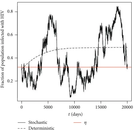
Example 10(𝑅𝑆₀> 1). Let us use the same parameter values as in Example 8 but changing𝜇to0.125/year and thus3.42466×

10−4_{/day [4]. Let us define}_{𝜐 = 0.05}_{and thus}_𝑅𝐷

0 = 2.386057

and𝑅𝑆₀ = 1.1942 > 1. Therefore by Theorem 4, for any given initial value𝜋₀ = 𝜋(0) ∈ (0, 1), the solution𝜋(𝑡)for the SDE HIV model (14) should obey

lim

[image:10.600.314.541.70.294.2]

(11)

0 5000 10000 15000 20000 0.2

0.8

0.6

0.4

t (days)

Frac

tio

n

o

f p

op

u

la

tio

n

inf

ec

te

d wi

th

HIV

Stochastic Deterministic

[image:11.600.57.285.70.291.2]

𝜂

0 5000 10000 15000 20000 25000

0.3 0.6

0.5

0.4

t (days)

Frac

tio

n

o

f p

op

u

la

tio

n

inf

ec

ted wi

th

HIV

Stochastic Deterministic

[image:11.600.56.285.346.568.2]

𝜂

Figure 3 clearly supports our analytical results given in Theorem 4 by showing the solution path of𝜋(𝑡) oscillates around the level 𝜂 in finite time. Again the numerical simulations were repeated and the same conclusion can be drawn each time.

In order to further illustrate the effect of the noise intensity𝜐has on the solution, in the next example we will keep all the parameter values the same as in Example 10 but reducing the noise intensity.

Example 11. By keeping the parameter values the same as in Example 10 and reducing𝜐to 0.02, we have that𝑅𝐷₀ =

2.38605, 𝑅𝑆₀ = 2.195363 > 1, and 𝜂 = 0.4770654. By Theorem 4 and Proposition 5, we would expect the solution

𝜋(𝑡)to persist and oscillate around the level𝜂. Furthermore by Proposition 5, as𝜐 → 0, we would expect𝜂to tend towards the deterministic equilibrium value for the corresponding deterministic model given by (11); namely,(𝜐𝜎 − 𝜇𝜌)/(𝜐𝜎 −

𝜇𝜌 + 𝜇𝜏) = 0.4924476.

From Figure 4, we can clearly see that the solution path

𝜋(𝑡) does indeed oscillate about the level 𝜂. Moreover, by comparing Figures 3 and 4, we can also see that as we reduce the noise intensity from 0.05 to 0.02, the level𝜂does indeed tend towards the deterministic equilibrium value as expected.

In the next example we will use histograms to see how the solution of the SDE HIV model oscillates around the level𝜂 as we vary the noise intensity𝜐.

Example 12. Let us use the same parameter values as in Example 10 and choose𝜐 to be0.05,0.04, 0.03,0.005, and

0.001. We then let the simulations run for 1 million iterations but disregarding the first 800,000 iterations in order to allow

𝜋(𝑡)to reach its recurrent level.

From Figure 5, we can see from the histograms that, for larger 𝜐, the distribution of the solution is more skewed, while, for smaller 𝜐, the distribution is more normally distributed about the level𝜂. This is further confirmed by the sample skewness coefficients, namely, 1.000705, 0.4264459,

−0.3415049, 0.2185976, and0.003324568 corresponding to

𝜐 = 0.05,0.04,0.03,0.005, and0.001, respectively.

Furthermore, we have used the quantile-quantile plot (QQ plot) to further illustrate that, for the smaller values of

𝜐, these data are not far from being normally distributed. The result is shown in Figure 6.

8. Conclusion

(12)

De

n

si

ty

0.2 0.4 0.6

0 1 2 3 4 5 6 7

De

n

si

ty

0.50 0.60 0.70

0 2 4 6 8 10

De

n

si

ty

0.25 0.35 0.45

0 2 4 6 8 10

De

n

si

ty

0.46 0.48

0 20 40 60 80

De

n

si

ty

0.480 0.484 0.488

0 50 100 150 200 250

𝜋(t):𝜐 = 0.001

𝜋(t):𝜐 = 0.005

𝜋(t):𝜐 = 0.03

𝜋(t):𝜐 = 0.04

𝜋(t):𝜐 = 0.05

Figure 5: Histogram for the solution path𝜋(𝑡)for the SDE HIV model (14) with step sizeΔ = 0.01using parameter values given in Example 12 with initial value𝜋(0) = 0.3and𝜐 = 0.05, 0.04, 0.03, 0.005, and0.001.

0.480 0.482 0.484 0.486 0.488 0.490

−4−2 0 2 4

Theoretical quantiles

Sa

m

ple q

u

an

tiles:

𝜐

=

0.001

−4−2 0 2 4

0.25 0.30 0.35 0.40 0.45

Sa

m

ple q

u

an

tiles:

𝜐

=

0.03

0.465 0.470 0.475 0.480 0.485 0.490 0.495

Sa

m

ple q

u

an

tiles:

𝜐

=

0.005

−4−2 0 2 4

Figure 6: QQ plot for the solution path𝜋(𝑡)for the SDE HIV model (14) corresponding to the histograms shown in Figure 5 for𝜐 = 0.03, 0.005,

(13)

By using the well-known Khasminskii theorem, we have shown that the SDE HIV model has a unique stationary distribution. Lastly, numerical simulations using realistic parameter values are constructed to support our analytical results.

Note that𝑅𝑆₀has a natural interpretation as follows: if we consider introducing a single newly infected individual into the disease-free equilibrium (DFE) and consider the number of secondary cases that he or she produces, then near the DFE equation (14) becomes

𝑑𝜋 (𝑡) = 𝜋 (𝜐𝜎_𝜌 − 𝜇) 𝑑𝑡 +𝜐𝜎_𝜌𝜋𝑑𝐵, (91)

with solution

𝜋 (𝑡)

= 𝜋₀exp[{(𝜐𝜎

𝜌 − 𝜇) − 1 2

𝜐2_𝜎2

𝜌2 } 𝑡 +

𝜐𝜎 𝜌 𝐵 (𝑡)] .

(92)

Also lim_𝑡→∞|𝐵(𝑡)|/𝑡 = 0a.s. Hence we expect that if

𝑅𝑆₀= (𝜐𝜎 𝜇𝜌) −

𝜐2𝜎2

2𝜌2_𝜇 < 1, (93)

then the disease dies out whereas if 𝑅𝑆₀ > 1, the disease takes off. Thus this is a natural biological interpretation of the stochastic basic reproduction number𝑅𝑆₀.

Deterministic models have in the past proved very useful in describing the spread of HIV amongst PWIDs but they have their faults. The real world is stochastic and in general stochastic models are more realistic than deterministic ones. Recall that

2𝜌2_𝜇, (94)

where𝑅𝐷₀ represents the basic reproduction number in the deterministic model. So in the deterministic model𝑅𝐷₀ is the expected number of secondary cases caused by a single newly infected PWID entering a population consisting entirely of susceptible PWIDs and uninfected needles. The second term in (94) is an adjustment factor for the stochastic model.

In the deterministic model we have a straightforward scenario where if the basic reproduction number𝑅𝐷₀ ≤ 1, then it is known that the disease will die out, whereas if

𝑅𝐷

0 > 1, then the disease will persist. The results in this paper

show that, in the stochastic model, if𝑅𝑆₀< 1, then the disease dies out (almost surely), whereas if𝑅𝑆₀ > 1, then the disease ultimately persists and oscillates about a nonzero level. These theoretical results are confirmed by numerical simulations. Moreover the argument above shows that if a single newly infected PWID enters the DFE, then we expect the disease to die out if𝑅𝑆₀< 1and take off if𝑅𝑆₀> 1.

These findings provide new insights into the spread of HIV amongst PWIDs. Because the stochastic basic repro-duction number𝑅₀𝑆is less than the deterministic one, it is possible for the noise to drive the disease to extinction, that

is, if𝑅𝐷₀ > 1, so that in the deterministic model the disease will persist; then if the stochastic noise is large enough, in the stochastic model the disease will die out. This has important implications for control strategies. Deterministic models have often been used to predict control strategies, for example, the fraction of PWIDs who must clean their needles after use, the effects of HIV testing, or the amount that PWIDs need to decrease their syringe sharing rates in order to reduce𝑅𝐷₀ beneath one and eliminate disease. Examples of this applied to HIV amongst PWIDs include Greenhalgh and Lewis [32], Lewis [33] as well as Lewis and Greenhalgh [34]. Examples applied to hepatitis C virus (HCV) control include Corson [35] and Corson et al. [23].

The analytical and numerical results of this paper provide new insight into this. If there is significant stochastic noise in the system, then these estimates will be overestimated; that is, a smaller fraction of PWIDs cleaning their needles or a smaller reduction in PWID syringe sharing rates will still be sufficient for elimination of disease transmission.

Disclosure

The research data associated with this paper which was funded by EPSRC is available at http://dx.doi.org/10.15129/ bf5ba8b5-d484-43c7-8006-14fb76819be2.

Conflict of Interests

The authors declare that there is no conflict of interests regarding the publication of this paper.

Acknowledgments

Yanfeng Liang is grateful to the EPSRC for a studentship to support this work (EPSRC DTP Grant Reference no. EP/K503174/1) and the authors are grateful for the R coding provided by Drs. Alison Gray and Jiafeng Pan, Department of Mathematics and Statistics, University of Strathclyde, Glasgow, UK, which allowed the authors to modify the code to create the simulations shown in this paper. David Green-halgh is grateful to the Leverhulme Trust for support from a Leverhulme Research Fellowship (RF-2015-88). Xuerong Mao is grateful to the Leverhulme Trust (RF-2015-385) and the Royal Society of London (IE131408) for their financial support.

References

[1] World Health Organization, “Global Health Observatory Data,” September 2015, http://www.who.int/gho/hiv/en/.

[2] World Health Organization, Media Centre, September 2015, http://www.who/int/mediacentre/factsheets/fs360/en/. [3] World Health Organization, “HIV/AIDS,” September 2015,

http://www.who.int/hiv/topics/idu/en/.

(14)

[5] D. Greenhalgh and G. Hay, “Mathematical modelling of the spread of HIV/AIDS amongst injecting drug users,” IMA Journal of Mathemathics Applied in Medicine and Biology, vol. 14, no. 1, pp. 11–38, 1997.

[6] S. M. Blower, D. Hartel, H. Dowlatabadi, R. M. Anderson, and R. M. May, “Drugs, sex and HIV: a mathematical model for New York City,”Philosophical Transactions of the Royal Society B: Biological Sciences, vol. 331, no. 1260, pp. 171–187, 1991. [7] J. P. Caulkins and E. H. Kaplan, “AIDS impact on the number

of intravenous drug users,”Interfaces, vol. 21, no. 3, pp. 50–63, 1991.

[8] F. Lewis and D. Greenhalgh, “Three stage AIDS incubation period: a worst case scenario using addict-needle interaction assumptions,”Mathematical Biosciences, vol. 169, no. 1, pp. 53– 87, 2001.

[9] D. Greenhalgh and F. Lewis, “The general mixing of addicts and needles in a variable-infectivity needle-sharing environment,” Journal of Mathematical Biology, vol. 44, no. 6, pp. 561–598, 2002.

[10] E. H. Kaplan and E. O’Keefe, “Let the needles do the talking! evaluating the new haven needle exchange,”Interfaces, vol. 23, no. 1, pp. 7–26, 1993.

[11] F. Lewis and D. Greenhalgh, “Three stage AIDS incubation period: a worst case scenario using addict-needle interaction assumptions,”Mathematical Biosciences, vol. 169, no. 1, pp. 53– 87, 2001.

[12] T. Rhodes, M. Singer, P. Bourgois, S. R. Friedman, and S. A. Strathdee, “The social structure production of HIV risk among injecting drug users,”Journal of Social Science and Medicine, vol. 61, no. 5, pp. 1026–1044, 2005.

[13] Y. Ding, M. Xu, and L. Hu, “Risk analysis for AIDS control based on a stochastic model with treatment rate,”Human and Ecological Risk Assessment, vol. 15, no. 4, pp. 765–777, 2009. [14] G. R. Gupta, J. O. Parkhurst, J. A. Ogden, P. Aggleton, and A.

Mahal, “Structural approaches to HIV prevention,”The Lancet, vol. 372, no. 9640, pp. 764–775, 2008.

[15] S. A. Strathdee, T. B. Hallett, N. Bobrova et al., “HIV and risk environment for injecting drug users: the past, present, and future,”The Lancet, vol. 376, no. 9737, pp. 268–284, 2010. [16] N. Dalal, D. Greenhalgh, and X. Mao, “A stochastic model for

internal HIV dynamics,”Journal of Mathematical Analysis and Applications, vol. 341, no. 2, pp. 1084–1101, 2008.

[17] H. C. Tuckwell and E. Le Corfec, “A stochastic model for early HIV-1 population dynamics,”Journal of Theoretical Biology, vol. 195, no. 4, pp. 451–463, 1998.

[18] N. Dalal, D. Greenhalgh, and X. Mao, “A stochastic model of AIDS and condom use,”Journal of Mathematical Analysis and Applications, vol. 325, no. 1, pp. 36–53, 2007.

[19] D. Peterson, K. Willard, M. Altmann, L. Gatewood, and G. Davidson, “Monte Carlo simulation of HIV infection in an intravenous drug user community,”Journal of Acquired Immune Deficiency Syndromes, vol. 3, no. 11, pp. 1086–1095, 1990. [20] D. Greenhalgh and F. Lewis, “Stochastic models for the spread of

HIV amongst in-travenous drug users,”Stochastic Models, vol. 17, no. 4, pp. 491–512, 2001.

[21] A. Gray, D. Greenhalgh, L. Hu, X. Mao, and J. Pan, “A stochastic differential equation SIS epidemic model,”SIAM Journal on Applied Mathematics, vol. 71, no. 3, pp. 876–902, 2011.

[22] Z. Huang, Q. Yang, and J. Cao, “Complex dynamics in a stochastic internal HIV model,”Chaos, Solitons & Fractals, vol. 44, no. 11, pp. 954–963, 2011.

[23] S. W. Corson, D. Greenhalgh, and S. Hutchinson, “Mathemati-cally modelling the spread of hepatitis C in injecting drug users,” Mathematical Medicine and Biology, vol. 29, no. 3, pp. 205–230, 2012.

[24] S. W. Corson, D. Greenhalgh, and S. J. Hutchinson, “A time since onset of injection model for hepatitis C spread amongst injecting drug users,”Journal of Mathematical Biology, vol. 66, no. 4-5, pp. 935–978, 2013.

[25] Q. Lu, “Stability of SIRS system with random perturbations,” Physica A: Statistical Mechanics and Its Applications, vol. 388, no. 18, pp. 3677–3686, 2009.

[26] X. Mao, G. Marion, and E. Renshaw, “Environmental Brownian noise suppresses explosions in population dynamics,”Stochastic Processes and Their Applications, vol. 97, no. 1, pp. 95–110, 2002. [27] Q. Yang, D. Jiang, N. Shi, and C. Ji, “The ergodicity and extinction of stochastically perturbed SIR and SEIR epidemic models with saturated incidence,” Journal of Mathematical Analysis and Applications, vol. 388, no. 1, pp. 248–271, 2012. [28] Q. Yang and X. Mao, “Extinction and recurrence of

multi-group SEIR epidemic models with stochastic perturbations,” Nonlinear Analysis: Real World Applications, vol. 14, no. 3, pp. 1434–1456, 2013.

[29] E. Tornatore, S. M. Buccellato, and P. Vetro, “Stability of a stochastic SIR system,”Physica A: Statistical Mechanics and its Applications, vol. 354, pp. 111–126, 2005.

[30] X. Mao, Stochastic Differential Equations and Applications, Horwood, Chichester, UK, 2nd edition, 2008.

[31] R. Z. Khasminskii,Stochastic Stability of Differential Equations, Sijthoff & Noordhoff, Alphen aan den Rijn, The Netherlands, 1980.

[32] D. Greenhalgh and F. Lewis, “Modelling the spread of AIDS among intravenous drug users including variable infectivity, HIV testing and needle exchange,”Journal of Medical Informat-ics and Technologies, vol. 2, no. 1, pp. IP3–IP11, 2001.

[33] F. I. Lewis,Assessing the impact of variable infectivity on the transmission of HIV amongst intravenous drug users [Ph.D. thesis], University of Strathclyde, Glasgow, UK, 2000.

[34] F. Lewis and D. Greenhalgh, “HIV testing as an effective control strategy against the spread of AIDS among intravenous drug users,”Archives of Control Sciences, vol. 9, no. 1-2, pp. 69–96, 1999.

(15)

Submit your manuscripts at

http://www.hindawi.com

Stem Cells

International

Hindawi Publishing Corporation

http://www.hindawi.com Volume 2014

INFLAMMATION

Behavioural

Neurology

Endocrinology

International Journal of

Disease Markers

BioMed

Research International

Oncology

Journal of

http://www.hindawi.com Volume 2014 Oxidative Medicine and Cellular Longevity Hindawi Publishing Corporation

PPAR Research

The Scientific

World Journal

Immunology Research

Journal of

Obesity

Journal of

http://www.hindawi.com Volume 2014 Computational and Mathematical Methods in Medicine

Ophthalmology

Journal of

Diabetes Research

Journal of

http://www.hindawi.com Volume 2014 Research and Treatment

AIDS

Gastroenterology Research and Practice

Parkinson’s

Disease

Evidence-Based Complementary and Alternative Medicine

Volume 2014