City, University of London Institutional Repository
Citation
:
Fernandez-Perez, A., Fuertes, A. & Miffre, J. (2016). Commodity Markets, Long-Run Predictability and Intertemporal Pricing. Review of Finance, doi:https://doi.org/10.1093/rof/rfw034
This is the accepted version of the paper.
This version of the publication may differ from the final published
version.
Permanent repository link:
http://openaccess.city.ac.uk/13601/Link to published version
:
https://doi.org/10.1093/rof/rfw034Copyright and reuse:
City Research Online aims to make research
outputs of City, University of London available to a wider audience.
Copyright and Moral Rights remain with the author(s) and/or copyright
holders. URLs from City Research Online may be freely distributed and
linked to.
City Research Online: http://openaccess.city.ac.uk/ [email protected]
1
Commodity Markets, Long-Run Predictability and Intertemporal Pricing
ADRIAN FERNANDEZ-PEREZ1, ANA-MARIA FUERTES2, JOELLE MIFFRE3
Review of Finance (forthcoming)
Abstract
This paper shows that commodity portfolios that capture the backwardation and contango phases exhibit in-sample and out-of-sample predictive power for the first two moments of the distribution of long-horizon aggregate equity market returns, and for the business cycle. It also demonstrates that a pricing model based on the corresponding backwardation and contango risk factors explains relatively well a wide cross-section of equity portfolios. The cross-sectional “hedging” risk prices are economically consistent with the direction of long-horizon predictability. Backwardation and contango thus act as plausible investment opportunity state variables in the context of Merton’s (1973) intertemporal CAPM.
Keywords: Commodities; Backwardation; Contango; Long-Run Predictability; Intertemporal
Pricing
JEL classifications: G13, G14
_______________
1 Auckland University of Technology, Department of Finance, Private Bag 92006, 1142 Auckland, New Zealand. Phone: +64 9 921 9999; e-mail: [email protected].
2 Cass Business School, City University London, Faculty of Finance, ECIY 8TZ, London, England; Tel: +44 (0)20 7040 0186; e-mail: [email protected]. Corresponding author.
3 EDHEC Business School, 392 Promenade des Anglais, Nice, France; Tel: +33 (0)4 9318 3255; e-mail: [email protected].
2
Commodity Markets, Long-Run Predictability and Intertemporal Pricing
Abstract
This paper shows that commodity portfolios that capture the backwardation and contango
phases exhibit in-sample and out-of-sample predictive power for the first two moments of the
distribution of long-horizon aggregate equity market returns, and for the business cycle. It also
demonstrates that a pricing model based on the corresponding backwardation and contango risk
factors explains relatively well a wide cross-section of equity portfolios. The cross-sectional
“hedging” risk prices are economically consistent with the direction of long-horizon
predictability. Backwardation and contango thus act as plausible investment opportunity state
variables in the context of Merton’s (1973) intertemporal CAPM.
Keywords: Commodities; Backwardation; Contango; Long-Run Predictability; Intertemporal
Pricing
3
1. Introduction
The literature on commodity futures pricing centers around the concepts of backwardation and
contango as formalized in the theory of storage (Kaldor, 1939; Working, 1949; Brennan, 1958)
and the hedging pressure hypothesis (Keynes, 1930; Cootner, 1960; Hirshleifer, 1988). Returns
of backwardated and contangoed portfolios have been shown to explain the cross-section of
commodity futures returns (e.g., Basu and Miffre, 2013; Szymanowskaet al., 2014; Bakshiet
al., 2015). The purpose of this article is to investigate whether those returns tell us anything
about long-run changes in investment opportunities and intertemporal asset pricing.
The theory of storage explains the dynamics of commodity futures prices by linking the
slope of their term structure (hereafter, TS) to agents’ incentive to hold the physical commodity.
With high inventories, the term structure slopes upward, futures prices are expected to fall with
maturity, and markets are contangoed. Conversely, when inventories are depleted, the utility
from holding the physical asset (convenience yield) exceeds storage and financing costs; the
futures curve then slopes downward, futures prices are expected to rise with maturity, and
markets are backwardated. Fama and French (1987) document that the basis or gap between
futures and spot prices depends on interest rates and seasonals in convenience yields. Erb and
Harvey (2006), Gorton and Rouwenhorst (2006) and Gorton et al. (2012) also support the theory
of storage by showing that the risk premium of commodity futures is driven by the basis and
inventory levels.1
1 There are also competitive rational expectations models of storage in a risk-neutral setting where the
non-negativity constraint on inventory is crucial to understanding the dynamics of the spot price and the
shape of the forward curve (Deaton and Laroque, 1992; Routledge et al., 2000). Extensions that allow
4
The hedging pressure hypothesis instead attempts to explain the behavior of commodity
futures prices with reference to the net positions of hedgers and speculators. Futures prices are
predicted to increase when hedgers are net short and speculators are net long; markets are then
in backwardation. Conversely, futures prices are expected to fall when hedgers are net long and
speculators net short; markets are in contango.Hedging pressure (hereafter, HP) has been
shown to play a key role as driver of commodity futures risk premia (Carter et al., 1983;
Bessembinder, 1992; de Roon et al., 2000; Basu and Miffre, 2013).2
Commodity price momentum (hereafter, Mom) can be linked with backwardation and
contango through the theory of storage. Deviations of inventories from normal levels are likely
to persist as inventories can only be replenished through new production which may take time
depending on the commodity. Thus, following a negative shock to inventories which increases
the spot price, a period of high expected futures risk premia will follow as inventories are
gradually restored. Gorton et al. (2012) present evidence to support this view.
The returns of commodity portfolios based on backwardation and contango signals (such
as TS, HP and Mom) can thus be interpreted as a compensation for bearing risk during times
when the futures curves slope downwards, when inventories are low and/or when hedgers are
net short. Using as proxy for the investment opportunity set the aggregate equity market, this
article documents that backwardation and contango contain predictiveinformation about future
2 The sharp increase in commodity assets under management post-2004 revived the debate on the
function of speculators as both liquidity and risk-bearing providers, and on their potential influence on
futures prices, volatility and cross-market linkages (Stoll and Whaley, 2010; Brunetti et al., 2013;
Büyükşahin and Robe, 2014). Theoretical models explain the recent swings in storable commodity prices in terms of endogenous demand shocks and changes in supply fundamentals; see, e.g. Baker and
5
changes in investment opportunities that is not fully revealed by traditional predictors (such as
the dividend yield or term spread). This aligns well with our parallel finding that the
backwardation and contango portfolios can also predict economic activity as proxied by real
GDP growth of the G7 economies. Our analysis confirms that the predictive power of
backwardation and contango over future changes in investment opportunities is strong at long
horizons. This empirical finding dovetails neatly with the low frequency (or business cycle)
dynamics of expected market returns and market volatility.
These predictability findings motivate us to estimate a novel version of Merton’s (1973)
Intertemporal Capital Asset Pricing Model (ICAPM) using as risk factors the innovations to the
TS, HP and Mom state variables. We show that these innovations are priced risk factors in the
cross-section of stock returns, and further demonstrate that the signs of the risk prices are
economically consistent with the direction of long-horizon predictability. The results agree with
the notion that rational investors are willing to pay a higher price on stocks that hedge
intertemporal risk, and demand a lower price on stocks that are unable to hedge because they
underperform when market conditions are predicted to deteriorate. The proposed commodity
factor model is able to price quite well the cross-section of stock returns, compared to extant
ICAPM implementations in the literature. The predictive ability of backwardation and contango
thus translates into dynamic risk premia in equity markets.
Our findings are robust to various checks. The long-run predictive ability of the
backwardation and contango state variables for future changes in investment opportunities is
not challenged when we consider alternative statistical tests, different out-of-sample forecast
evaluation periods, and rolling versus recursive forecasting schemes. The finding that
innovations to the commodity state variables are priced factors in the cross-section of stock
6
is robust to altering the set of test assets and the ICAPM formulation to account for recursive
preferences à-la Epstein and Zin (1989, 1991).
Our study relates to an extensive literature on equity premium predictability that draws
upon a variety of macroeconomic and equity-based variables; see recent surveys by Cochrane
(2011) and Rapach and Zhou (2013). It also speaks to a new commodity markets literature that
suggests that the backwardation and contango cycle plays a role as leading indicator of future
economic activity (Baker and Routledge, 2012; Koijen et al., 2013; Bakshi et al., 2015).3 Other
recent studies show that commodity market variables such as the returns of commodity futures,
open interest, oil supply/demand shocks or the Baltic Dry Index explain the cross-section of
equity returns or predict the business cycle (Hong and Yogo, 2012; Bakshi et al., 2012; Hou
and Szymanowska, 2013; Ready, 2014a; Boons et al., 2014). Our paper extends these studies
by showing that backwardation and contango state variables have additional predictive content
(beyond traditional predictors) for long-run changes in the investment opportunity set, and that
this predictive ability translates into “hedging” risk premia for the cross-section of equities.
The paper unfolds as follows. Section 2 outlines the background theory. Section 3 describes
the data and methodology to construct the commodity state variables. Sections 4 and 5 report
the main empirical results and robustness checks. Section 6 concludes.
2. Market Return Predictability and Intertemporal Asset Pricing
The fundamental insight of intertemporal asset pricing theory is that, in solving their lifetime
consumption decisions under uncertainty, long-term investors care not only about the current
3 Baker and Routledge (2012) show that bond excess returns are higher when the crude oil futures curve
slopes downward. Bakshi et al. (2015) document that commodity TS and Mom portfolios forecast real
GDP growth and traditional asset returns. Koijen et al. (2013) show that the TS strategy performs well
7
level of their invested wealth but also about the future returns on that wealth. Merton’s (1973)
ICAPM in discrete time and logarithmic form can be expressed as follows
, = , + ∆ , , = 1, … , (1)
where (∙) is a conditional expectation, , is the month to + 1 excess return of asset ,
is the market portfolio that proxies the investment opportunity set, ∆ is an innovation in the
state variable that predicts changes in future investment opportunities, and , is a
conditional covariance. In equilibrium, the expected excess return on asset is dictated by its
covariance with current returns on total invested wealth, , , and with news about future
returns on invested wealth, ∆ , . The prices of market and intertemporal risks are captured by
and , respectively.4 If investors do not care about future long-horizon investment
opportunities, = 0, or if the investment opportunity set is constant over time, ∆ , = 0, then
the expected return-covariance Equation (1) becomes the static CAPM.
Merton’s (1973) theory does not, however, identify the state variables and so it could be
applied as a “fishing license” (Fama, 1991) for ad-hoc risk factors. Yet, as Cochrane (2005)
forcefully argues, the problem is not with the theory itself but with bad habits of applying the
theory. More to the point, two restrictions that emanate from the theory ought to be tested.
The first restriction concerns the time-series behavior of the state variables; namely, they
must be able to predict long-horizon changes in investment opportunities. Since these changes
4 can be interpreted as the representative investor’s relative risk aversion (RRA) in this simplified
ICAPM setting that assumes time-additive expected utility and is also adopted by Hahn and Lee (2006),
Petkova (2006), Bali and Engle (2010), Maio and Santa-Clara (2012) and others. However, this
interpretation is not appropriate in ICAPMs built upon the recursive preferences of Epstein and Zin
8
can be driven by the first or second moments of the aggregate market return distribution, we
estimate as in Maio and Santa-Clara (2012) the following pair of predictive regressions
, : = + ′ + : , (2)
, : = + ′ + : , (3)
by ordinary least squares (OLS) with monthly data = 1, … , where is the effective sample
size. The target variable in Equation (2) is the market portfolio excess return continuously
compounded from months + 1 to + ℎ; namely, , : ≡ , + ⋯ + , . The target
variable in Equation (3) is the sum of monthly realized variances, , : ≡ , + ⋯ +
, , where , is the sum of squared daily market excess returns on month + 1. The candidate set of predictors is collected in the state vector ≡ ( , , … , , )′.
The second restriction links the time-series behavior of the state variables and the
cross-sectional behavior of the “hedging” risk factors. If a state variable , has predictive slopes
> 0 in (2) and < 0 in (3), then negative innovations in , predict a deterioration in the
investment opportunity set, and the intertemporal price of risk associated with , should be
positive; > 0 in (1). Intuitively, assets that perform poorly when investment opportunities
are predicted to worsen are undesirable because they reduce the agent’s ability to hedge
intertemporal risk; those assets should command a positive risk premium in equilibrium.
Likewise, the predictive slopes < 0 and > 0 in (2) and (3) go hand-in-hand with a
negative intertemporal risk price < 0 in (1).
Following Campbell (1996), Petkova (2006), Maio (2013) and others, we construct the
intertemporal risk factors through the following vector autoregressive (VAR) model
, = + , −
− + ,, , (4)
which is estimated by OLS with monthly data = 1, … , ; and are the sample means of
9
vector , , suitably orthogonalized with respect to , and standardized so that they have
the same standard deviation as ̂ , , are our proxies for the intertemporal risk factors.
Let the vector ≡ ( , ,…, , )′ denote the intertemporal risk factors thus
constructed. Then we estimate the covariance risk prices in Equation (1) by the generalized
method of moments (GMM) approach developed by Hansen (1982). The GMM system is
( ) =1 ,, −− , , − − ′ , ( − ) −
= (5)
where the first moment conditions are the pricing errors for risky portfolios = 1, … , , and
the remaining + 1 conditions account for the uncertainty associated with estimating the
means of all the factors ( , ′). The main parameters of interest in ≡ ( , ′, , ′)′ are
the market risk price and the intertemporal “hedging” risk prices ≡ ( , … , )′.
3. Variables and Data Description
The sample period is January 1987 to August 2011 ( = 296 months) and the start is dictated
by the availability of data on large hedgers and speculators positions in the Commitment of
Traders report published by the U.S. Commodity Futures Trading Commission (CFTC).
3.1 COMMODITY AND TRADITIONAL STATE VARIABLES
Our leading conjecture is that the backwardation and contango cycle present in commodity
futures markets has predictive content for the first two moments of long-horizon aggregate
equity market returns. To test it, we construct backwardation and contango mimicking
portfolios from end-of-month settlement prices of futures contracts for 27 commodities from
Datastream; 12 agricultural products (cocoa, coffee C, corn, cotton n°2, frozen concentrated
orange juice, oats, rough rice, soybean meal, soybean oil, soybeans, sugar n°11, wheat), 5
energies (electricity, gasoline, heating oil, light sweet crude oil, natural gas), 4 livestock (feeder
10
silver), and lumber. Returns are computed for each commodity using the front-end contract
until one month before the maturity date, the positions are then rolled to the 2nd nearest contract.
The backwardation and contango mimicking portfolios systematically buy the 20% of
commodity futures that are most backwardated and short the 20% of commodity futures that
are most contangoed. The commodity futures in both the long and short portfolios are
equally-weighted. The fully-collateralized long-short portfolios are held for one month, and the sorting
is carried out again. This sequential sorting is based on a moving average of term structure (TS),
hedging pressure (HP) or momentum (Mom) signals. We entertain a long 12-month moving
average to capture the slow dynamics of inventories (Gorton et al., 2012).
The TS signal is the roll yield or differential between the logarithmic prices of front and
second nearest contracts; thus, the TS portfolio buys the assets with the highest average
roll-yields and shorts the assets with the lowest average roll roll-yields. The HP signal for the ith
commodity combines the hedging pressure of hedgers ( ,) and hedging pressure of
speculators ( , ) defined as , ≡ ,
, , and , ≡
,
, , where
, denotes the open interest of long hedgers, ℎ , denotes the open interest of short hedgers, and so forth.5 Accordingly, following the Basu and Miffre (2013) approach, the HP
portfolio buys the backwardated contracts with the lowest average , values and the highest
average , values, and it shorts the contangoed contracts with the highest average ,
5 The CFTC classifies commodity traders as reportable or non-reportable according to the size of their
positions (large or small, respectively). Reportable traders have to state whether they act as commercial
hedgers or non-commercial speculators and whether they take long or short positions. These declarations
are checked, summarized in the Aggregated Commitment of Traders Report and published on the CFTC
website on a bi-monthly or weekly basis. The corresponding open interest time-series made available
11
values and lowest average , values. The Mom signal of the ith commodity is its past average
excess return; thus, the Mom portfolio buys the commodity futures contracts with the highest
mean excess returns and shorts the contracts with the lowest mean excess returns.
We benchmark the predictive ability of commodity state variables (and the cross-sectional
pricing ability of innovations to the state variables) against traditional predictors. The
traditional state variables are inspired from extant intertemporal asset pricing models that can
be grouped as follows. On the one hand, we have the multifactor models proposed by Fama and
French (1993), Carhart (1997) and Pastor and Stambaugh (2003), that were not conceived as
applications of Merton’s (1973) theory but have been interpreted as such later on. Here the state
variables are the returns of equity portfolios sorted on size (SMB), value (HML) and momentum
(UMD), together with a liquidity risk factor (L). Then we have five popular ICAPM applications
that employ traditional macroeconomic variables; e.g. the models proposed by Campbell and
Vuolteenaho (2004), Hahn and Lee (2006), Petkova (2006), Bali and Engle (2010) and Koijen
et al. (2014). Appendix A provides further details on the traditional state variables.
As in Maio and Santa-Clara (2012), the predictive regressions (2) and (3) employ the
cumulative sums of UMD and L (from months t to t-59) as predictors in order to match the
persistence of the target variables and the other (macroeconomic) predictors. The same
transformation is made for SMB, HML and the commodity state variables; e.g. ≡
∑ where denotes the month excess return of the TS factor-mimicking portfolio.
3.2 MARKET PORTFOLIO AND TEST ASSETS
The market portfolio is proxied by the U.S. value-weighted equity index from Kenneth French’s
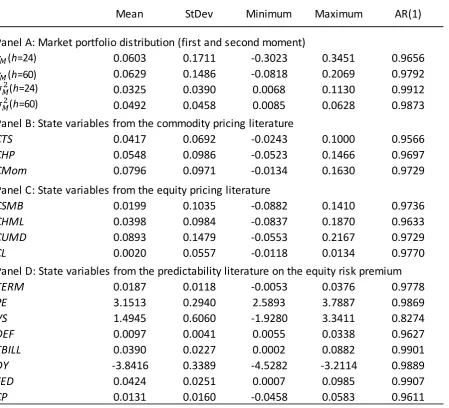
library. Table I presents summary statistics for the first two moments of the distribution of
monthly equity market excess returns (Panel A), and likewise for the candidate predictors
(Panels B to D); all returns are logarithmic and annualized. The average equity risk premium is
12
Sharpe ratio of 0.37. Aggregate stock market returns and variance at 24- and 60-month horizons
are persistent (akin to macroeconomic variables such as the default or term spread) with
first-order autocorrelation coefficients above 0.96. The cumulated empirical commodity and equity
state variables show a similar degree of persistence. The correlations between the commodity
state variables are positive but low (0.33 at most) which warrants their joint consideration. The
test assets for the cross-sectional pricing exercise are CRSP NYSE/AMEX/NASDAQ stocks
sorted on size and book-to-market (25 portfolios) from Kenneth French’s library.
[Insert Table I around here]
4. Empirical Results
4.1 LONG-RUN PREDICTABILITY
Do the commodity state variables predict long-run changes in investment opportunities? This
section begins by addressing this question through a standard in-sample analysis of
predictability; namely, the predictive regressions are estimated by OLS using the full sample.
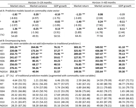
Table II presents estimation results for predictive regressions (2) and (3) at horizons ℎ of
24 and 60 months. Panel A reports predictive slopes together with Newey and West (1987)
significance t-ratios and ² statistics for the regressions based on the commodity state vector
≡ ( , , )′. Reassuringly, the freely estimated predictive slopes in (2)
and (3) have opposite signs. The 54% ² (h=24) and 64% ² (h=60) for the market return
equation indicates an economically large degree of predictability at long horizons; likewise for
the market variance. Hence, commodity state variables are able to forecast long-run changes in
investment opportunities. But do they add predictive power to traditional predictors?
[Insert Table II around here]
To address this question, the traditional predictive regressions are augmented with the
commodity state vector ( ) and we formally test the null hypothesis that traditional
13
against the alternative hypothesis that the corresponding vector of commodity slopes is not
identically zero. The Wald test statistics reported in Panel B of Table II are generally large and
strongly reject this hypothesis at the 1% level or better.
Aligned with the above test results, as shown in Panel C of Table II, the commodity state
variables notably enhance the predictive ability (in-sample ²) of traditional state variables for
the future aggregate market return and variance, Equations (2) and (3), respectively.
Specifically, by adding commodity state variables to traditional specifications of regression (2),
their predictive ability rises from 25% to 66% on average. Likewise, the ² of the variance
regression (3) more than doubles from 33% to 68% on average across specifications. The
regression slopes (and t-ratios) tabulated in Appendix B for the traditional state variables
confirm extant evidence that they can predict long-run changes in investment opportunities
(Cochrane, 2005; Maio and Santa-Clara, 2012; Rapach et al., 2010). Altogether, the results
shown in Panels B and C of Table II indicate that commodity state variables contain information
on future changes in investment opportunities that is not fully revealed by known predictors;
untabulated results for horizons h={12, 36} confirm this novel finding.
Does the additional predictive ability of the commodity state variables (over traditional
predictors) relate to their information content on macroeconomic risk? To address this question,
we fit by OLS the predictive regression log ( / ) = + ′ + : to
quarterly G7 real GDP data (obtained from Datastream); the commodity and traditional
predictors are sampled quarterly here and the predictive horizons are ℎ = {8, 20} to match those
in the preceding monthly regressions. The results reported in columns three and six of Table II
confirm that commodity state variables convey additional information (beyond that contained
in traditional predictors) to anticipate long-run changes in future economic conditions.
Thus far the results suggest that the backwardation and contango phases of commodity
14
opportunities. Yet in order to provide firm evidence, we should shield our predictive analysis
from two caveats. One is the Stambaugh (1999) bias that distorts t- and Wald-tests based on
standard asymptotic critical values when the predictors are highly persistent; i.e., the Type I
error (probability of wrongly rejecting the null hypothesis) is inflated. We construct their
empirical critical values by subsampling using the Romano and Wolf (2001)
minimum-volatility block size selection method. Significance according to the subsampling (asymptotic)
tests is denoted with asterisks (bold font) in Table II and Appendix B. The subsampling-based
Wald test inferences still suggest that the commodity state variables proposed are not
encompassed by traditional predictors.
The other potential caveat is look-ahead bias or the problem that in-sample predictability
may not translate into predictability in real time (see, e.g. Welch and Goyal, 2008). We address
this issue by estimating Equations (2) and (3) recursively over expanding windows in order to
construct two sequences of = (1 3⁄ ) out-of-sample (OOS, hereafter) for the future
aggregate equity market return and variance, ̂ , : and , : , respectively.
Table III sets out the comparison of OOS predictive ability of commodity and traditional
state variables. The evaluation criteria are the mean absolute error = ∑ | ̂ : |
and mean square error = ∑ ̂ : where ̂ : ≡ : − : is the
OOS forecasting error and the target variable is the aggregate market return or variance. The
table reports the t-statistics of Diebold and Mariano (1995) for the null hypothesis:
: ∆ = − = 0 (versus : ∆ ≠ 0) and likewise for the MSE
criterion. It also displays the of Campbell and Thompson (2008) that gives the
proportional reduction in mean squared errors that a given forecasting model attainsversus the
historical average benchmark. More specifically, = 1 − where =
15
assumptions of no predictability of the first and second moment of aggregate equity market
returns; these assumptions amount to imposing = 0 in (2) and ′ = 0 in (3), respectively.
The hypothesis that a predictive model yields smaller MSE than the historical average,
: ≤ 0 (against : > 0), is examined by the one-sided t-test of Clark and West
(2007) for nested models. All tests control for autocorrelation in prediction errors à-la Newey
and West (1987).6 The results suggest that the predictive regressions (2) and (3) based on
commodity state variables often yield significantly lower MAE, lower MSE and higher
than traditional regressions, particularly, at the longest horizon of 60 months.7
[Insert Table III around here]
The Clark and West (2007) t-statistic is also used to conduct two encompassing tests called
and for brevity. is a test of the null hypothesis that forecasts from
a traditional model are as accurate as forecasts from the same model augmented with
commodity variables; the alternative hypothesis is that the commodity state variables add
forecast accuracy ( : − ≤ 0 against : − > 0). The
notation is used to denote an otherwise identical test to assess the reverse statement
that commodity predictors encompass traditional predictors. Table III shows the MSE-adjusted
t-statistics pertaining to these hypotheses. For the aggregate market return, Equation (2), the
overall findings from both encompassing tests are that commodity state variables add
significant predictive information to traditional state variables but not the other way round. The
6 The size distortions related to the Stambaugh bias are not of concern in tests of out-of-sample predictive
ability; e.g., see Busetti and Marcucci (2012).
7 The high predictive ability of 56% for the commodity-based predictive model is clearly linked
to the long horizon as borne out by the fact that it falls to 37% at a 24-month horizon; untabulated results
16
evidence is inconclusive for the aggregate market variance, Equation (3); those models for
which the test is insignificant, the test is also insignificant. Untabulated
results for the tests applied to the out-of-sample predictions of real GDP growth at the
8 and 20 quarter-ahead horizons indicate, like the in-sample results shown in Table II, that
commodity state variables add predictive information content to traditional state variables;
detailed results are available from the authors upon request.
Altogether the in-sample and out-of-sample analyses suggest that the backwardation and
contango state variables have long-horizon predictive ability for the first two moments of the
distribution of aggregate market excess returns, and for changes in economic conditions. Next
we examine whether this predictability translates into intertemporal risk premia.
4.2 CROSS-SECTIONAL INTERTEMPORAL PRICING
Using the 25 equity test portfolios outlined in Section 3.2, we estimate the expected
return-covariance Equation (1) by GMM. The intertemporal risk factors are innovations to either
commodity state variables or to traditional state variables. The estimation results are shown in
Table IV. Are the signs of the intertemporal risk prices consistent with the signs of the long-run
predictive slopes? The negative risk prices and reported in Panel A are aligned with
the negative predictive slopes and for the long-run aggregate equity market return, and
with the positive slopes and for the long-run aggregate equity market variance (c.f.,
Table II). This confirms that rational agents are prepared to pay higher prices on assets that
hedge intertemporal risk. Likewise, the positive risk price is consistent with the positive
(negative) link between the Mom state variable and the mean (variance) of the future aggregate
market return distribution. This shows that rational investors require a positive premium on
assets that are poor hedges against future changes in the investment opportunity set.
17
In contrast, the intertemporal risk prices obtained for the traditional state variables in Panels
B and C of Table IV are in most cases economically incompatible with the direction of
time-series predictability which reaffirms the evidence in Maio and Santa-Clara (2012). To illustrate,
a decrease in term spread (TERM) anticipates a worsening of long-run investment opportunities
as borne out by the signs of the time-series slopes reported in Appendix B. Hence, assets that
covary positively with innovations to TERM do not hedge reinvestment risk and a positive
premium is expected; conflictingly, the cross-sectional risk price is negative.8
Next we assess the ability of the various pricing models to capture the cross-sectional
variation in the average excess returns of the N test portfolios. For this purpose, we average the
pricing errors ≡ , and calculate the = ∑ | | and =
∑ statistics, as well as the degrees-of-freedom adjusted fraction of the cross-sectional
variation in average excess returns captured by the pricing model, = 1 − ( )( ̅ ). We also
deploy the test statistic = [ ] for the null hypothesis that the sum of squared pricing
errors is zero where ≡ ( , … , ) , and is the first × block of the spectral density
matrix of the moment conditions. Finally, for each pricing model Figure 1 presents a scatterplot
of the portfolios’ average excess return and the model-based expected excess return. As borne
out by the results in Table IV and Figure 1 the commodity risk factor model compares well with
8 The RRA levels implied by our market risk price estimates, ranging from 2.19 to 3.16 across models,
are in line with those documented in previous studies; see e.g., Mehra and Prescott (1985), Cochrane
(2005), Bali and Engle (2010), Maio and Santa-Clara (2012) and Campbell et al. (2015). However, they
represent small RRA levels relative to the predictions stemming from expected-utility theory (see, e.g.
18
traditional multifactor models in terms of pricing ability.9 The commodity state variables
capture relatively well the “hedging” risk premia that agents demand on equities.
[Insert Figure 1 around here]
5. Sensitivity Analysis
This section adds robustness to our findings regarding the roles of commodity state variables
as predictors of changes in investment opportunities and as drivers of intertemporal risk.
First, we analyze the predictive ability of commodity and traditional state variables under a
rolling (instead of recursive or expanding window) forecasting scheme that estimates the
models over windows of fixed length = (2 3⁄ ) months where is the total sample size.
Rolling estimation is appealing because it offers a ‘shield’ against structural breaks in the data.
Second, we repeat the recursive predictive analysis by considering a long holdout or
out-of-sample period = (1 2⁄ ) beginning on May 1999, instead of = (1 3⁄ ) beginning on
June 2003 as until now. Table V summarizes the results of both robustness checks through a
subset of the measures reported in Table III; the unreported measures do not alter the main
findings. The efficacy of the commodity state variables as OOS predictors of future changes in
investment opportunities is not challenged when we obtain the forecasts through rolling
estimation of the predictive regressions, nor when the forecast evaluation period is lengthened.
[Insert Table V around here]
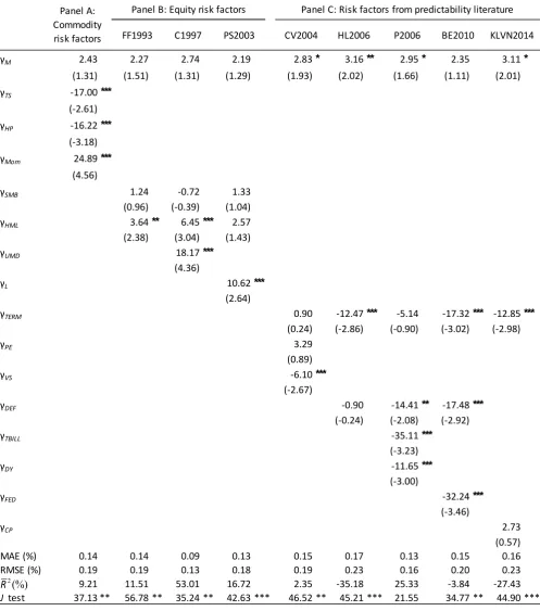
Turning now to the cross-sectional leg of our investigation, we conduct the pricing analysis
for the commodity-based and traditional multifactor models using as test assets the 25 equity
portfolios sorted on size and momentum available from Kenneth French’s library. The results
9 In line with Maio and Santa-Clara (2012), the CAPM has no pricing ability as suggested by a negative
19
presented in Appendix C confirm our earlier conclusions. In the commodity-based ICAPM
specification of Panel A, the signs of the intertemporal risk prices are consistent with the
direction of long-horizon predictability; in contrast, this restriction is violated for many of the
traditional models (Panels B and C). This suggests that, unlike traditional predictors, the
commodity factor mimicking portfolios act as economically plausible candidates for investment
opportunity state variables in the Merton (1973) ICAPM theory. Moreover, in practical terms,
the proposed pricing model based on commodity risk factors competes well with traditional
ICAPM implementations in terms of cross-sectional pricing ability.
We implement also the ICAPM of Campbell (1993, 1996) that is formulated upon Epstein
and Zin (1989, 1991) preferences together with a log-linear approximation of the representative
agent’s budget constraint. The expected return-covariance equation can be expressed as
, + , ⁄ =2 , + ( − 1) ∑ , (6)
where , ⁄2 is a Jensen’s inequality adjustment due to log-normality; is interpreted as the
investor’s RRA level; and , denotes the ith asset covariance with innovations in the market
portfolio returns (for = 1) and with innovations in the commodity TS, HP and Mom state
variables ( = 2, 3 and 4 respectively), where the latter act as proxies for news about future
changes on invested wealth. The relative importance of the market return and the commodity
state variables in forecasting future investment opportunities is captured by the elements of the
vector ≡ ( , , , ). In this setting, the risk prices are no longer freely estimated
but restricted instead to maintain a particular relation with and the RRA parameter; namely,
≡ + ( − 1) , and ≡ ( − 1) for = { , , }. Using the 25 size and
book-to-market value portfolios as test assets, the GMM estimation of this restricted ICAPM
formulation yields significant risk prices of -49.06 (t-stat of -4.03), of -23.99 (t-stat of
20
long-horizon predictability. This confirms that the innovations to the backwardation and
contango state variables act as plausible intertemporal “hedging” risk factors.10
6. Conclusions
Motivated by the theory of storage and the hedging pressure hypothesis, we construct
backwardation and contango state variables as factor-mimicking commodity portfolio returns
using term structure, hedging pressure and momentum signals. Our findings show that the
commodity state variables contain predictive information for future long-run changes in
investment opportunities (and for the business cycle) that is not fully revealed by traditional
state variables such as the dividend yield, default spread or term spread. The results hold both
in- and out-of-sample, for different forecasting schemes, horizons and evaluation periods.
These findings lead us to examine whether the innovations in the commodity state variables
are priced risk factors in a novel ICAPM formulation. We show that the cross-sectional risk
prices associated with innovations to the commodity state variables are significant and
economically consistent with the direction of long-run predictability. An ICAPM specification
based on the commodity risk factors alone can explain the cross-sectional variation in equity
returns relatively well. The predictive ability of the backwardation and contango state variables
for aggregate equity market returns (variance) and business-cycle fluctuations is thus shown to
be consistent with the intertemporal “hedging” risk premia that rational agents demand on
equities.
10 It is worth stressing that in our setting the basket of commodities is not intended to proxy for the
“single good” consumed by the representative investor in the Epstein and Zin (1989, 1991) recursive
preferences framework. The commodities allow us to construct the backwardation and contango state
variables that convey information about the future returns on aggregate wealth. The RRA level implied
21
The paper adds to a new literature that ascribes a role to commodity market variables, such
as the basis and open interest, as leading indicators of economic activity and sources of priced
risk in equities. Our findings could stimulate further research on the relation between the equity
22 APPENDIX A. Description of traditional state variables
Panel I outlines the multifactor models that have been interpreted as applications of Merton’s (1973) ICAPM theory. Definitions and sources for each of the state variables are provided in Panel II. All the variables are sampled at a monthly frequency. CV2004 is an unrestricted version of Campbell and Vuolteenaho (2004).
Panel I: Multifactor models
Fama and French (FF1993)
SMB √ √ √
HML √ √ √
UMD √
L √
TERM √ √ √ √ √
PE √
VS √
DEF √ √ √
TBILL √
DY √
FED √
CP √
Panel II: Description of state variables
SMB Size factor (difference in returns between small and large capitalization stocks) K.R. French's website
HML Value factor (difference in returns between high and low book-to-market stocks) K.R. French's website
UMD Equity momentum factor (difference in returns between winner and loser stocks) K.R. French's website
L Innovations in aggregate liquidity constructed by Pastor and Stambaugh (2003) R. F. Stambaugh's website
TERM Slope of Treasury yield curve (yield spread between the 10 year T-bond and 3 month T-bill) US Federal Reserve website
PE Price earnings (ratio of the price of the S&P 500 index to a ten-year moving average of earnings) R. Shiller's website
VS Value spread (difference between the log book-to-market ratios of small-value and small-growth stocks) K.R. French's website
DEF Default spread (difference between the yields on BAA- and AAA-rated corporate bonds) US Federal Reserve website
TBILL 3-month T-bill rate US Federal Reserve website
DY Dividend yield (ratio of the sum of annual dividends to the level of the S&P 500 index) Bloomberg
FED Federal reserve fund rate US Federal Reserve website
CP Cochrane-Piazzesi (2005) bond factor obtained as the fitted value from a regression of excess bond returns on forward rates M. Piazzesi's website
A. State variables from equity pricing literature B. State variables from predictability literature
Koijen et al.
(KLVN2014) Bali and Engle
(BE2010) Petkova
(P2006) Hahn and Lee
23 APPENDIX B. Long-run predictive regressions of future aggregate market returns and market variances using traditional state variables
The table reports OLS regression estimation results for future aggregate market returns (Panel A) and realized market variances at 24- and 60-months horizons using traditional predictors in various sets as employed in existing models; see Appendix A for details. The market portfolio is proxied by the U.S. value-weighted stock index from Kenneth French’s library. All regressions include an (unreported) intercept. Bold denotes significance at the conventional 10%, 5% or 1% levels according to the asymptotic Student’s t critical values using the Newey-West adjustment. *, **, *** denote significance at the 10%, 5% and 1% levels according to subsampling critical values computed using the Romano and Wolf (2001) minimum-volatility block selection method. The estimation period is January 1987 to August 2011.
Horizon h=24 months
CSMB -0.21 -0.17 -0.11 0.00 -0.02 0.00
CHML 0.43 0.49 0.44 -0.04 -0.06 -0.04
CUMD 0.25 -0.11**
CL 0.13 0.00
TERM 5.15 10.20 6.72 13.35*** 6.82 -2.00 -2.73** -2.46*** -2.61* -0.43
PE -0.40 0.01
VS 0.00 0.00
DEF 1.50 2.00 7.30 5.29** 5.00** 5.52**
TBILL 0.90 -0.24
DY 0.36 -0.04
FED 3.38 0.13
CP 0.05 -0.03**
Horizon h=60 months
CSMB -0.31 -0.35 -0.13 0.04 0.06 0.08
CHML 0.04 0.22 0.07 0.09 0.02 0.10
CUMD 0.41 -0.18**
CL 0.21*** 0.05
TERM -3.13 16.04*** 9.34*** 32.35*** 5.96 -3.16* -4.09 -5.80*** -7.46*** -3.00
PE -1.27 0.07
VS 0.03 -0.01
DEF -38.37 65.65** 24.53 -0.90 -15.12** -13.92*
TBILL 12.30*** -3.30**
DY 0.96*** -0.05
FED 18.46*** -3.82**
CP 0.12 -0.02
CV2004
BE2010 KLVN2014 FF1993 C1997 PS2003
P2006
Panel A: Market return Panel B: Market variance
24 APPENDIX C. Robustness of cross-sectional pricing results to choice of test assets
The table reports GMM estimation results for an ICAPM based on the commodity TS, HP and Mom factors (Panel A) and traditional ICAPM representations (Panels B and C; see Appendix A for details). The test assets are 25 equity portfolios sorted on size and momentum. is the market (covariance) risk price, and the remaining coefficients are the intertemporal covariance risk prices associated with the “hedging” risk factors. Robust GMM t-statistics are reported (in parentheses) based on the Bartlett kernel with Newey-West optimal bandwidth selection. The performance metrics are mean absolute pricing error (MAE), root mean square error (RMSE), degrees-of-freedom adjusted fraction of the cross-sectional variance in average excess returns explained by the model ( ), and test statistic for the null hypothesis that the sum of squared pricing errors is zero which follows asymptotically a ( ) where N and K+1 are the number of testing assets and model risk factors, respectively. *, ** and *** denote significance at the 10%, 5% and 1% levels, respectively. The sample period is January 1987 to August 2011.
γM 3.14* 2.00 2.86* 1.88 3.23* 3.98** 3.72** 3.40** 2.96 (1.75) (1.41) (1.76) (0.77) (1.90) (2.26) (2.13) (2.02) (1.50)
γTS -9.51* (-1.65)
γHP -13.91** (-2.33)
γMom 22.84*** (3.18)
γSMB 2.16 0.84 1.33
(1.52) (0.55) (0.68)
γHML 0.83 4.48** -3.54
(0.42) (2.10) (-0.92)
γUMD 4.24**
(2.41)
γL 35.55***
(3.37)
γTERM -16.71*** -12.22*** -19.75*** -14.71*** -8.75* (-3.84) (-2.98) (-4.12) (-3.67) (-1.92)
γPE 4.04
(0.82)
γVS 9.00**
(2.23)
γDEF -14.42** -15.30** -17.38**
(-2.09) (-2.37) (-2.46)
γTBILL -14.14**
(-2.66)
γDY 6.20
(1.31)
γFED -17.57***
(-3.25)
γCP 26.74***
(4.05)
MAE (%) 0.13 0.28 0.10 0.18 0.16 0.16 0.15 0.14 0.14
RMSE (%) 0.16 0.34 0.14 0.22 0.20 0.22 0.21 0.18 0.19
63.32 -48.16 73.39 32.23 42.57 34.20 34.49 55.75 52.96 J test 28.98 57.20 ** 47.03 ** 21.24 21.57 31.32 * 33.88 ** 34.02** 27.48
Panel A: Commodity risk factors
Panel B: Equity risk factors Panel C: Risk factors from predictability literature
FF1993 C1997 PS2003 CV2004 HL2006 P2006 BE2010 KVLN2014
2(%)
25
References
Baker, S. (2014) The financialization of storable commodities, unpublished working paper,
Carnegie Mellon University.
Baker, S. and Routledge, B. (2012) The price of oil risk, unpublished working paper, Carnegie
Mellon University.
Bakshi, G., Gao, X. and Rossi, A. (2015) Understanding the sources of risk underlying the
cross-section of commodity returns, unpublished working paper, University of Maryland.
Bakshi, G., Panayotov, G. and Skoulakis, G. (2012) The Baltic Dry Index as a predictor of
global stock returns, Commodity Returns, and Global Economic Activity, unpublished
working paper, University of Maryland, Hong Kong University of Science & Technology,
University of British Columbia.
Bali, T. and Engle, R. (2010) The intertemporal capital asset pricing model with dynamic
conditional correlations, Journal of Monetary Economics57, 377-390.
Basu, D. and Miffre, J. (2013) Capturing the risk premium of commodity futures: the role of
hedging pressure, Journal of Banking and Finance37, 2652-2664.
Bessembinder, H. (1992) Systematic risk, hedging pressure, and risk premia in futures markets,
Review of Financial Studies5, 637-667.
Boons, M., de Roon, F. and Szymanowska, M. (2014) The price of commodity risk in stock
and futures markets, unpublished working paper, Nova School of Business and
Economics, Tilburg University, Erasmus University Rotterdam.
Brennan, M. (1958) The supply of storage, American Economic Review48, 50-72.
Brunetti, C., Büyükşahin, B. and Harris, J. (2013) Herding and speculation in the crude oil
market, Energy Journal34, 83-104.
Busetti, F. and Marcucci, J. (2012) Comparing forecast accuracy: a Monte Carlo investigation,
26
Büyükşahin, B. and Robe, M. (2014) Speculators, commodities and cross-market linkages,
Journal of International Money and Finance42, 38-70.
Campbell, J. (1993) Intertemporal asset pricing without consumption data, American Economic
Review83, 487–512.
Campbell, J. (1996) Understanding risk and return, Journal of Political Economy 104, 298–
345.
Campbell, J., Giglio, S., Polk, C. and Turley, R. (2015) An intertemporal CAPM with
stochastic volatility, unpublished working paper, Harvard University, University of
Chicago, London School of Economics.
Campbell, J. and Thompson, S. (2008) Predicting the equity premium out of sample: can
anything beat the historical average?, Review of Financial Studies21, 1509-1531.
Campbell, J. and Vuolteenaho, T. (2004) Bad beta, good beta, American Economic Review94,
1249-1275.
Carhart, M. (1997) On persistence in mutual fund performance, Journal of Finance52, 57-82.
Carter, C., Rausser, G. and Schmitz, A. (1983) Efficient asset portfolios and the theory of
normal backwardation, Journal of Political Economy91, 319-331.
Casassus, J., Collin-Dufresne, P. and Routledge, B. R. (2009) Equilibrium commodity prices
with irreversible investment and non-linear technologies, unpublished working paper,
Pontificia Universidad Catolica de Chile, Ecole Polytechnique Fédérale de Lausanne,
Carnegie Mellon University.
Clark, T. E. and West, K. D. (2007) Approximately normal tests for equal predictive accuracy
in nested models, Journal of Econometrics138, 291-311.
Cochrane, J. H. (2005) Asset Pricing, Princeton University Press, New Jersey, 2nd edition.
27
Cochrane, J. H. and Piazzesi, M. (2005) Bond risk premia, American Economic Review 95,
138–160.
Cootner, P. (1960) Returns to speculators: Telser vs. Keynes, Journal of Political Economy68,
396–404.
Deaton, A. and Laroque, G. (1992) On the behaviour of commodity prices, Review of Economic
Studies59, 1-23.
De Roon, F. A., Nijman, T. E. and Veld, C. (2000) Hedging pressure effects in futures markets,
Journal of Finance55, 1437-1456.
Diebold, F. X. and Mariano, R. S. (1995) Comparing predictive accuracy, Journal of Business
& Economic Statistics13, 253-263.
Epstein, L. and Zin, S. (1989) Substitution, risk aversion and the temporal behavior of
consumption and asset returns: A theoretical framework, Econometrica57, 937-969.
Epstein, L. and Zin, S. (1991) Substitution, risk aversion, and the temporal behavior of
consumption and asset returns: An empirical analysis, Journal of Political Economy99,
263-286.
Erb, C. and Harvey, C. (2006) The strategic and tactical value of commodity futures, Financial
Analysts Journal62, 69-97.
Fama, E. (1991) Efficient capital markets: II, Journal of Finance46, 1575–1617.
Fama, E. and French, K. (1987) Commodity futures prices: some evidence on forecast power,
premiums, and the theory of storage, Journal of Business60, 55-73.
Fama, E. and French, K. (1993) Common risk factors in the returns on stocks and bonds,
Journal of Financial Economics33, 3-56.
Gorton, G. and Rouwenhorst, G. (2006) Facts and fantasies about commodity futures,
28
Gorton, G., Hayashi, F. and Rouwenhorst, G. (2012) The fundamentals of commodity futures
returns, Review of Finance17, 35-105.
Hahn, J. and Lee, H. (2006) Yield spreads as alternative risk factors for size and
book-to-market, Journal of Financial and Quantitative Analysis41, 245-269.
Hansen, L. (1982) Large sample properties of generalized method of moments estimators,
Econometrica 50, 1029-1054.
Hirshleifer, D. (1988) Residual risk, trading costs, and commodity futures risk premia, Review
of Financial Studies1, 173-193.
Hong, H. and Yogo, M. (2012) What does futures market interest tell us about the
macroeconomy and asset prices?, Journal of Financial Economics105, 473–490.
Hou, K. and Szymanowska, M. (2013) Commodity-based consumption tracking portfolio and
the cross-section of average stock returns, unpublished working paper, Ohio State
University, Erasmus University Rotterdam.
Kaldor, N. (1939) Speculation and economic stability, Review of Economic Studies7, 1-27.
Keynes, M. (1930) A Treatise on Money II: The Applied Theory of Money, Edition Macmillan
and Co.
Koijen, R., Lustig, H. and Van Nieuwerburgh, S. (2014) The cross-section and time-series of
stock and bond returns, unpublished working paper, London Business School, Stanford
Graduate School of Business, New York University Stern School of Business.
Koijen, R., Moskowitz, T., Pedersen, L. and Vrugt., B. (2013) Carry, unpublished working
paper, London Business School, University of Chicago, Copenhagen Business School, VU
University Amsterdam.
Maio, P. (2013) Intertemporal CAPM with conditioning variables, Management Science59,
29
Maio, P. and Santa-Clara, P. (2012) Multifactor models and their consistency with the ICAPM,
Journal of Financial Economics106, 586–613.
Mehra, R. and Prescott, E. (1985) The equity premium: a puzzle, Journal of Monetary
Economics15, 145–161.
Mehra, R., (2003) The equity premium: why is it a puzzle?, Financial Analysts Journal59,
54-69.
Merton, R.C. (1973) An intertemporal capital asset pricing model, Econometrica41, 867-887.
Newey, W. K. and West, K. D. (1987) Hypothesis testing with efficient method of moments
estimation, International Economic Review28, 777-787.
Pastor, L. and Stambaugh, R. F. (2003) Liquidity risk and expected stock returns, Journal of
Political Economy111, 642-685.
Petkova, R. G. (2006) Do the Fama-French factors proxy for innovations in predictive
variables?, Journal of Finance61, 581-612.
Rabin, M. (2000) Risk aversion and expected-utility theory: a calibration theorem,
Econometrica68, 1281-1292.
Rapach, D. E. and Zhou, G. (2013) Forecasting stock returns, in: G. Elliott and A.
Timmermann, (eds.) Handbook of Economic Forecasting2A, Elsevier, Amsterdam,
328-383.
Rapach, D. E., Strauss, J. K. and Zhou, G. (2010) Out-of-sample equity premium prediction:
combination forecasts and links to the real economy, Review of Financial Studies23,
821-862.
Ready, R. (2014a) Oil prices and the stock market, unpublished working paper, University of
Rochester.
Ready, R. (2014b) Oil consumption, economic growth, and oil futures: a fundamental
30
Romano, J. and Wolf, M., (2001) Subsampling intervals in autoregressive models with linear
time trend, Econometrica69, 1283-1314.
Routledge, B. R., Seppi, D. J. and Spatt, C. S. (2000) Equilibrium forward curves for
commodities, Journal of Finance55, 1297-1338.
Stambaugh, R. F. (1999) Predictive regressions, Journal of Financial Economics54, 375-421.
Stoll, H. and Whaley, R. (2010) Commodity index investing and commodity futures prices,
Journal of Applied Finance20, 7-46.
Szymanowska, M., De Roon, F., Nijman, T. and Van Den Goorbergh, R. (2014) An anatomy
of commodity futures risk premia, Journal of Finance69, 453-482.
Welch, I. and Goyal, A. (2008) A comprehensive look at the empirical performance of equity
premium predictions, Review of Financial Studies64, 1067-1084.
31
Figure 1. Individual pricing errors of nine candidate ICAPMs
This figure plots the average excess return in percentage per annum (p.a.) of each test asset versus the corresponding prediction from each of nine ICAPMs. The test assets are 25 equity portfolios sorted on size and book-to-market. The sample period is January 1987 to August 2011. The commodity-based ICAPM employs as risk factors the market portfolio and innovations in the commodity TS, HP and Mom state variables. The remaining models are described in Appendix A.
32 Table I. Summary statistics for variables in predictability regressions
Panel A summarizes the target variables in predictive regressions (2) and (3), respectively, the aggregate excess market portfolio return and realized variance from month t+1 to t+h with h={24, 60} months. The market portfolio is proxied by the U.S. value-weighted stock index and the risk-free rate by the one-month Treasury-bill rate. The empirical state variables in Panel B and C are expressed in cumulated from month t to t-59. Panel B presents summary statistics for the backwardation and contango state variables constructed according to term structure (CTS), hedging pressure (CHP) and momentum (CMom) signals; Section 3.1 of the paper gives details on the construction of the commodity state variables. Panel C summarizes the equity size (CSMB) and value (CHML) portfolios of Fama and French (1993), the momentum (CUMD) portfolio of Carhart (1997) and the liquidity variable of Pastor and Stambaugh (2003; CL). Panel D reports state variables from the predictability literature. Appendix A gives details on the variables of Panels C and D. AR(1) is the first order autoregressive coefficient. All returns are annualized. The sample period is January 1987 to August 2011.
Mean StDev Minimum Maximum AR(1)
Panel A: Market portfolio distribution (first and second moment)
0.0603 0.1711 -0.3023 0.3451 0.9656
0.0629 0.1486 -0.0818 0.2069 0.9792
0.0325 0.0390 0.0068 0.1130 0.9912
0.0492 0.0458 0.0085 0.0628 0.9873
Panel B: State variables from the commodity pricing literature
CTS 0.0417 0.0692 -0.0243 0.1000 0.9566
CHP 0.0548 0.0986 -0.0523 0.1466 0.9697
CMom 0.0796 0.0971 -0.0134 0.1630 0.9729
Panel C: State variables from the equity pricing literature
CSMB 0.0199 0.1035 -0.0882 0.1410 0.9736
CHML 0.0398 0.0984 -0.0837 0.1870 0.9633
CUMD 0.0893 0.1479 -0.0553 0.2167 0.9729
CL 0.0020 0.0557 -0.0118 0.0134 0.9770
Panel D: State variables from the predictability literature on the equity risk premium
TERM 0.0187 0.0118 -0.0053 0.0376 0.9778
PE 3.1513 0.2940 2.5893 3.7887 0.9869
VS 1.4945 0.6060 -1.9280 3.3411 0.8274
DEF 0.0097 0.0041 0.0055 0.0338 0.9627
TBILL 0.0390 0.0227 0.0002 0.0882 0.9901
DY -3.8416 0.3389 -4.5282 -3.2114 0.9889
FED 0.0424 0.0251 0.0007 0.0985 0.9907
CP 0.0131 0.0160 -0.0458 0.0583 0.9611
33 Table II. Long-run predictive regressions for future aggregate market returns and variances
Panel A reports in the first two columns of each section the OLS estimation results of regressions (2) and (3) at horizons of 24 and 60 months ahead; the predictors are the cumulated commodity factor-mimicking portfolio returns,
≡ ( , , )′. The third column reports quarterly OLS predictive regressions for G7 real GDP
growth, ∆ : ≡ log ( / ), at counterpart horizons of 8 and 20 quarters ahead. All regressions include an unreported intercept. Newey-West (1987) t-test statistics are shown in parentheses. Panel B reports Wald encompassing test statistics for traditional predictive regressions augmented with ; the null hypothesis is that traditional predictors encompass commodity predictors, e.g., : = = = 0 in the augmented regressions. Panel C reports the adjusted R2 (%) of traditional predictive regressions and augmented versions. The market portfolio is proxied by the U.S. value-weighted stock index from Kenneth French’s library. Section 3 and Appendix A provides detailed definitions of commodity and traditional state variables. Bold denotes significance at the 10%, 5% or 1% levels according to the asymptotic distribution. *, **, *** denote significance at the 10%, 5% and 1% levels according to the subsampling distribution based on the minimum-volatility block selection method of Romano and Wolf (2001). The estimation period is January 1987 to August 2011.
Panel A: Predictive models based on commodity state vector
CTS -1.82*** 0.20* -0.10*** -1.23*** 0.08 -0.09
(-8.83) (4.97) (-3.75) (-3.69) (2.04) (-1.62)
CHP -0.18** 0.10* -0.02*** -1.40*** 0.24*** -0.11*
(-2.07) (4.32) (-2.09) (-9.39) (7.90) (-3.30)
CMom 1.36*** -0.25 *** 0.13*** 1.34*** -0.21*** 0.11*
(8.68) (-5.36) (3.91) (5.89) (-6.78) (2.44)
54.69 49.91 50.55 64.41 77.56 35.47
Panel B: Encompassing tests
(H0: commodity state variables do not add information to traditional predictors)
FF1993 245.24*** 264.06 *** 76.31** 303.31*** 549.92*** 61.10*** C1997 220.08*** 173.34 *** 37.27** 325.92*** 436.08*** 59.26*** PS2003 232.73*** 277.47 *** 74.96*** 289.69*** 507.47*** 79.13*** CV2004 241.67*** 140.09 *** 59.61** 127.91*** 269.41*** 51.44** HL2006 284.47*** 80.35* 44.23* 211.92*** 353.90*** 44.93** P2006 256.03*** 68.17** 48.53 76.85*** 390.82*** 38.35* BE2010 276.41*** 94.26** 43.34* 143.40*** 349.69*** 43.50 KLVN2014 253.22*** 40.94 31.57 149.56*** 235.64*** 59.30** Panel C: of traditional predictive models (augmented with commodity state variables)
FF1993 4.64 (55.72) 1.21 (55.96) 6.46 (55.33) 2.59 (64.26) 14.59 (79.39) 43.87 (72.71) C1997 9.39 (55.55) 20.51 (56.20) 34.77 (57.07) 5.83 (67.15) 32.40 (80.70) 48.77 (74.91) PS2003 7.43 (55.90) 0.74 (57.09) 5.74 (54.90) 6.89 (64.96) 20.11 (79.60) 51.16 (79.73) CV2004 29.01 (66.86) 18.43 (50.74) 13.22 (53.29) 58.06 (75.64) 44.82 (78.27) 1.65 (48.16) HL2006 20.32 (65.95) 34.50 (52.13) 17.69 (49.05) 21.82 (64.48) 41.11 (80.48) 3.64 (45.33) P2006 31.43 (69.06) 37.24 (52.21) 18.25 (51.92) 73.53 (81.48) 60.27 (87.79) 44.69 (66.82) BE2010 21.21 (65.87) 34.23 (54.22) 16.61 (48.24) 41.00 (67.43) 61.83 (87.29) 48.74 (70.71) KLVN2014 28.25 (67.26) 58.28 (64.66) 35.16 (54.54) 33.96 (64.16) 49.08 (78.21) 3.86 (52.49)
Horizon h=24 months Horizon h=60 months
GDP growth Market return Market variance GDP growth Market return Market variance
%
34
Table III. Out-of-sample predictions for long-run future aggregate market returns and variances
The table summarizes the out-of-sample (OOS) forecasts of predictive regressions (2) and (3) at horizons of 24 and 60 months. The state variables are described in Section 3 and Appendix A. ∆ (∆ ) refers to the Diebold and Mariano (1995) t-stat for the hypothesis of equality in mean absolute (squared) prediction errors between traditional and commodity models; e.g., : − = 0 versus : − ≠ 0. is the percentage reduction in MSE achieved by the predictive model versus the historical average benchmark; the Clark and West (2007) MSE-adjusted statistic is used to assess significance ( : ≤ 0 vs. : > 0). ( ) is the Clark and West (2007) MSE-adjusted t-stat for the null hypothesis that the forecasts from a traditional (commodity) model encompass the forecasts from the model augmented with commodity (traditional) predictors; e.g.,
: − ≤ 0 vs. : − > 0 for . *, **, *** indicates significant at the 10%, 5% and 1% levels. All tests are Newey-West adjusted for autocorrelation in prediction errors. The holdout period is June 2003 to August 2011 (T1=1/3T).
Model
Commodity 36.7** 56.5***
FF1993 6.32 *** 5.14*** -154.0 2.67*** 0.17 10.06*** 7.73*** -386.1 8.10*** 0.56
C1997 7.08 *** 5.67*** -360.5 6.09*** 0.39 10.73*** 8.29*** -328.1 4.16*** 0.49
PS2003 5.65 *** 4.86*** -128.5 1.52* -0.89 8.47*** 6.36*** -1650.6 6.30*** 0.44
CV2004 1.58 1.76* -45.8 -1.13 -0.07 2.45** 2.49** 23.1* 1.69** 2.38**
HL2006 2.79 *** 2.08** -78.6 2.79*** -0.67 1.66* 1.73* -27.6 2.16** -0.42
P2006 4.58 *** 3.78*** -115.3 0.70 -0.89 0.40 0.57 36.1*** 3.25*** 3.73***
BE2010 2.70 *** 2.10** -91.4 2.75*** -0.60 1.38 1.40 10.7*** 1.89** 1.31*
-1.28 -0.31 40.0*** 2.70*** 2.58*** 1.71* 1.85* -19.9 2.93*** -2.07
Commodity 26.1** 76.7***
FF1993 -0.49 1.38 -9.2 3.40*** 1.23 3.40*** 3.36*** -23.9 2.23** -0.10
C1997 1.33 2.16** -50.6 5.01*** 1.14 2.83*** 2.90*** -2.0 1.39* -0.16
PS2003 -0.58 1.38 -11.2 2.62*** 1.17 9.27*** 6.13*** -970.9 5.91*** -0.15
CV2004 0.38 1.94* -25.7 -3.04 -0.75 3.16*** 3.34*** 11.9* 3.62*** 0.23
HL2006 -1.58 -0.56 30.8*** 0.28 -0.03 3.80*** 3.22*** -17.5 6.18*** 0.33
P2006 0.18 1.68* -15.6 -3.45 -1.06 3.26*** 3.80*** -2.8 6.24*** 2.11**
BE2010 -0.79 0.04 25.7*** 0.02 -0.51 4.35*** 3.37*** -33.2 5.10*** 0.23
-3.82 *** -3.14*** 45.0*** -3.65 1.66* 2.99*** 2.78*** 14.4* 7.56*** -0.16
ENCtrad ENCcomm
Panel A: Market return
Panel B: Market variance
KLVN2014 KLVN2014
ENCtrad ENCcomm
ΔMSE
ΔMAE
ΔMAE ΔMSE
Horizonh=24 months Horizon h=60 months