Multi-directional maximum-entropy approach to the evolutionary design optimization of water distribution systems

Multi-Directional Maximum-Entropy Approach

to the Evolutionary Design Optimization

of Water Distribution Systems

Salah Saleh1,2&Tiku T. Tanyimboh1

Received: 4 November 2015 / Accepted: 28 January 2016

#The Author(s) 2016. This article is published with open access at Springerlink.com

Abstract A new multi-directional search approach that aims at maximizing the flow entropy of water distribution systems is investigated. The aim is to develop an efficient and practical maximum entropy based approach. The resulting optimization problem has four objectives, and the merits of objective reduction in the computational solution of the problem are investigated also. The relationship between statistical flow entropy and hydraulic reliability/ failure tolerance is not monotonic. Consequently, a large number of maximum flow entropy solutions must be investigated to strike a balance between cost and hydraulic reliability. A

multi-objective evolutionary optimization model is developed that generatessimultaneously a

wide range of maximum entropy values along with clusters of maximum and near-maximum entropy solutions.Results for a benchmark network and a real network in the literature are included that demonstrate the effectiveness of the procedure.

Keywords Maximum flow entropy . Hydraulic reliability and redundancy . Water distribution system . Demand driven analysis . Head driven analysis . Penalty-free constrained evolutionary optimization

1 Introduction

In the context of the design of water distribution systems, the least cost feasible solution is marginally able to satisfy the hydraulic requirements. Thus any failure in any system compo-nent can significantly affect the hydraulic performance of such designs. The incorporation of criteria other than cost to distinguish further between feasible solutions would lead to the DOI 10.1007/s11269-016-1253-6

* Tiku T. Tanyimboh [email protected]

1

Department of Civil and Environmental Engineering, University of Strathclyde Glasgow, Level 5, James Weir Building, 75 Montrose Street, Glasgow G1 1XJ, UK

2

retention of some spare capacity in the design albeit with an increase in the construction cost. Water distribution system design is conventionally dealt with as the determination of the cheapest design that is able to supply consumers with sufficient amounts of water at the required pressures. This has the limitation that such a design relies on the uninterrupted availability of all the components making up the system. However, water distribution systems are subject to component failures. For example, pipe breakage could happen due to increased pressure or pipe diameters could become smaller because of encrustation and tuberculation on

the internal walls. These circumstances significantly affect water distribution system’s

capac-ity. As a result, water distribution systems should be designed to have some spare capaccapac-ity. The absence of an agreed definition of reliability for water distribution systems along with

the computational complexity associated with its evaluation (Wagner et al. 1988) led

re-searchers to suggest various alternative surrogate reliability measures that are easy to evaluate within an optimization framework. These measures include statistical entropy (Tanyimboh and

Templeman 1993a,b,c,d), resilience index (Todini2000), network resilience (Prasad and

Park2004), modified resilience index (Jayaram and Srinivasan2008) and surplus power factor

(Vaabel et al. 2006). It has been shown that flow entropy is more accurate than the other

measures (Reca et al.2008; Raad et al.2010; Baños et al.2011; Tanyimboh et al.2011; Wu et

al.2011; Saleh et al.2012; Greco et al.2012; Czajkowska and Tanyimboh2013; Liu et al.

2014; Gheisi and Naser2015).

Entropy is highly dependent on the pipe flow directions and so it is possible to achieve alternative designs delivering maximum entropy flows with different levels of compromise

between cost and reliability. Tanyimboh and Templeman (1993a,b) suggested designing water

distribution systems to deliver maximum entropy flows as they are more reliable and relatively inexpensive compared to traditional minimum-cost designs (Tanyimboh and Templeman

2000). Setiadi et al. (2005) found that the overall correlation between hydraulic reliability

and entropy is positive. Furthermore, Tanyimboh and Sheahan (2002) demonstrated that two

different layouts having the same maximum entropy value tend to have similar properties such as hydraulic reliability. However, a water distribution system has a large number of feasible and infeasible sets of flow directions and consequently the early studies maximized entropy by limiting the solution space using predefined flow directions. The complexity of the underlying combinatorial optimization problem may be illustrated by noting that a network with 20 pipes

has 220i.e. 1,048,576 sets of flow directions.

The global maximum entropy (GME) optimization for water distribution systems is a many-objective optimization problem, i.e. optimization problems with four objectives or more. The application of multi-objective evolutionary algorithms in the solution of many-objective optimization problems leads to additional challenges including: high computational cost; poor scalability of most available multi-objective evolutionary algorithms, for example, most designs will have the same rank as the number of objectives increases; and difficulty in visualizing the Pareto-optimal front, for example, identifying the non-dominated solutions

when more than four objectives are involved (Saxena et al.2013).

In this paper, a multi-objective evolutionary optimization approach is developed that generates simultaneously a wide range of maximum entropy values along with clusters of maximum and near-maximum entropy solutions. Unlike previous approaches (e.g. Tanyimboh and Templeman

2000) the new procedure developed here does not require the pipe flow directions to be specified

2 Flow Entropy Function for Water Distribution Systems

Shannon (1948) introduced the statistical entropy concept as a measure of the amount of

uncertainty associated with any probability distribution. A random variable may have

alterna-tive discrete values xi, i= 1,…, n,with probabilities p(xi),where nis the total number of

discrete valued alternatives. Thus

Xn

i¼1

p xð Þ ¼i 1;p xð Þi >0;∀i ð1Þ

Shannon’s statistical entropy function is

S¼−X n

i¼1

p xð Þi lnp xð Þi ð2Þ

whereSis the entropy. Tanyimboh and Templeman (1993a,b,c,d) developed the statistical

flow entropy function for water distribution systems

S¼S0þ

XN

i¼1PiSi ð3Þ

in whichS= flow entropy;S0= entropy of sources or external supplies;Si= entropy of nodei;

Pi= fraction of the total flow that the network supplies that reaches nodei; andN= number of

nodes in the network.

S0¼−

X

i∈I Q_0i

T ln Q_0i

T

ð4Þ

whereQ0i= the inflow at source nodei, Tis the total demand and the setIincludes all the

source nodes. Also,

Si¼− Q_i0

Ti

ln Qi0

Ti

−X

i j∈Ni

Qi j Ti

ln Qi j

Ti

i¼1; :::::;N ð5Þ

whereSiis the entropy of nodei;Qi0is the demand at nodei; Qijis volume flow rate in pipeij;

Nirepresents the pipe flows from node i; Tiis the total flow that reaches nodei; therefore

Pi=Ti/Tis the fraction of the total demand that reaches nodei.

3 Optimization Model

There are many maximum entropy designs as there are many maximum entropy values for any water distribution system. The reason is that the entropy depends on the pipe flow directions.

The multiplicity of local maximum entropy (LME) values was theprimarymotivation for the

new approach proposed here. The multi-directional search aims to maximize simultaneously the entropy of all the different sets of pipe flow directions. For each candidate solution the

actual entropy valueSand the corresponding maximum entropy value (i.e. the largest possible

value with the same flow directions) are determined. The distance betweenSand the local

maximum entropy (LME) value represents the local search direction for each candidate

between eachLMEvalue and the global maximum entropy (GME) value is minimized. The

distance between theLMEandGMEvalues represents theglobal search directionfor each

candidate solution. The entropy value of each new solution produced is calculated (Eqs.3–5);

and if the flow directions are new, the correspondingLMEis calculated also. TheGMEvalue is

updated whenever a larger value is found.

The overall problem formulation can be described by defining the four objectives driving

the search. The first objective is the initial construction costf1that is minimized.

f1¼

X

i j∈I J

f Li j;Di j

ð6Þ

where, for pipeij, LijandDijare the length and diameter, respectively; andIJrepresents the

pipes in the network. The water distribution system should satisfy both the conservation of mass and energy requirements. These constraints are met externally by employing the

hydraulic solver EPANET 2 (Rossman 2000). The minimum nodal residual pressure

constraints were combined with the two goals of flow entropy maximization, i.e. simul-taneously maximizing the entropy of each design based on its flow distribution and seeking the design that has the global maximum entropy value. This results in an objective

function that represents a deficit in the hydraulic performance; the deficitf2is minimized.

f2¼T H DþðLM E−SÞ þðGM E−LM EÞ; T H D¼

X

i∈O

max 0ð ; Hreqi −HiÞ ð7Þ

THDis the total head deficit, i.e. the sum of the deficits in the required residual heads at the

demand nodes;HiandHireqare the available and required heads at nodei,respectively; the set

Oincludes all the demand nodes;Sis the actual entropy of the particular solution as in Eq.3.

The required head is the head above which the nodal demand is satisfied in full. If the available

headHiis larger than or equal to the required headHireqat all the demand nodes, then the

solution is considered hydraulically feasible andTHDtakes a value of zero. The second term

(LME-S) represents the local entropy search. It has a value of zero when both the actual

entropy and the corresponding maximum entropyLMEvalues are equal. Minimizing(LME-S)

actually maximizes S. The third term (GME-LME) represents the global entropy search.

Minimizing (GME-LME) actually maximizes LME. The search process therefore favours

larger values of entropySandLME. f2takes a value of zero if and only if all of the three

search components are equal to zero. This criterion applies only to theGMEsolution that is

hydraulically feasible and has local and global entropy search components of zero. This

ensures that the global search for theGME solution is maintained in each generation. The

GMEvalue is dynamic, as it is updated each time a larger value is discovered.

The contributions of the second and third terms due to entropy inf2can be relatively small

if the nodal head deficit is large. This means that the hydraulic performance deficit objective focuses primarily on satisfying the minimum node pressure constraints for pressure-deficient solutions. By contrast, the contributions of the second and third terms are significant if a solution has sufficient pressure and is thus hydraulically feasible. Therefore, once a hydrau-lically infeasible solution becomes feasible by evolution through crossover and/or mutation, the optimization process then focuses on reducing both the local and global entropy deficits. In this way the multi-directional search carries out both the local and global optimization

processes simultaneously. In the authors’previous work flow entropy was explicitly handled

excessively on the global maximization of entropy without paying enough attention to local

maximization of entropy (Saleh and Tanyimboh2011,2012).

4 Computational Solution

We used the nondominated sorting genetic algorithm (NSGA) II (Deb et al. 2002). The

optimization problem may be summarized as follows.

Minimizef¼ðf1; f2ÞT ð8Þ

The decision variables are the pipe diameters to be selected within the domain of the available discrete pipe sizes. In each generation, each new solution is analysed with the

hydraulic simulator EPANET 2 (Rossman2000) and the resulting pipe flow rates are used

to calculate the entropyS. The calculation of the maximum entropy values LME requires

numerical nonlinear optimization. However, much simpler methods that are quick, non-iterative and do not involve numerical optimization directly have been developed (Ang and

Jowitt 2005a, b; Yassin-Kassab et al. 1999; Tanyimboh and Templeman 1993c). In the

examples in the next section, we used the simplified path entropy method (Ang and Jowitt 2005a,b) for the single-source network (Example 1 and 2) and theα-method (Yassin-Kassab

et al.1999) for the real-world network with two sources (Example 3). For a network that has

two sources theα-method reduces to the solution of a nonlinear equation with one unknown;

we used the bisection method (Burden and Faires2001; Press et al. 2003). We wrote the

procedures in C to calculate theLMEvalues.

The proposed multi-directional search strategy is penalty-free, i.e. the costs of infeasible solutions are not artificially increased by including penalty terms in the cost objective function. The penalty-free philosophy aims to avoid the need to design and calibrate penalty functions

through time-consuming trial runs of the optimization algorithm (Siew and Tanyimboh2012a,

b). Also, penalty-free methods have the advantage of maintaining infeasible solutions having

useful values of decision variables that may not be common in the feasible solutions, to help safeguard diversity in the gene pool.

5 Results and Discussion

Figure 1 shows the single-source network and multi-source real-world system from the

literature used to demonstrate the new procedure. Network 1 in Fig.1ahas been extensively

5.1 Example 1

Example 1 is a hypothetical network from the literature (Fig.1a). Awumah et al. (1990)

introduced this network that has been used previously in many studies concerned with

entropy including Awumah et al. (1991), Tanyimboh and Templeman (2000), Liu et al.

(2014), etc. The network has a single source, 12 nodes and 17 pipes. The total head at the

supply node is 100 m. The elevation and required residual head for all the demand nodes are zero and 30 m respectively. All pipes are 1000 m long and the Hazen-Williams roughness coefficient is 130. There are 12 commercial pipe diameters in millimetres as follows: 100, 125, 150, 200, 250, 300, 350, 400, 450, 500, 550 and 600. The pipe cost per

metre is £800D1.5whereDis the diameter in metres. With 17 pipes and 12 candidate pipe

diameters the solution space is 1217= 2.22 × 1018. A 4-bit binary string was used to

represent the decision variables. There were thus four redundant codes that were arbitrarily allocated to the largest pipe diameter. Alternative allocation methods are available

(Herrera et al.1998; Saleh and Tanyimboh2014). The mutation rate was 1/68 or 0.015,

based on the length of each solution that comprises 68 binary bits. On average 527,130 function evaluations or hydraulic simulations in EPANET 2 were required to achieve convergence in each optimization run. The average CPU time was 12.3 min.

Previously, the highest entropy values achieved for this network were 3.1830 at a cost

of £1.357 million (Tanyimboh and Setiadi2008) and 3.5928 at a cost of £2.126 million

(Saleh and Tanyimboh2012). It is worth emphasizing, however, that these solutions were

based oncontinuouspipe diameters. The first attempt to find the global maximum entropy

(a) (b)

Fig. 1 Topologies of the sample networks considered.aNetwork 1.bNetwork 2 [with pipe numbers in square

design for this network using discrete pipe diameters (Saleh and Tanyimboh 2011)

achieved 3.5583 at a cost of £3.010 million. A new superior GME solution withdiscrete

pipe diameters has been achieved here with ahigherentropy value of 3.5925 and alower

cost of £2.890 million. Also, the surplus pressure at the critical node of theGMEsolution

has been reducedhere to 29.113 m from 38.78 m in Saleh and Tanyimboh (2011). The

cheapestLMEsolution has been improved here also,raisingthe entropy value to 2.5942

andloweringthe cost to £1.182 million. The previous cheapestLMEsolution (Saleh and

Tanyimboh2011) had a cost of £1.288 million and entropy value of 2.5605.

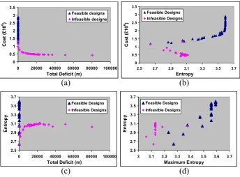
Also, the feasible solutions are well distributed in terms of cost (Fig. 2a) and entropy

(Fig. 2b and c). The simultaneous multi-directional search capability is evident from the

different maximum entropy clusters in Fig.2d. However, referring to the infeasible solutions

in Fig.2b, the relationship between cost and entropy should be treated with degree of caution

as the cost seems to decrease as the entropy increases. The apparent cost reduction could be due to the demand-driven simulation model that assumes the demands are satisfied even if

pressure is not sufficient. Furthermore Fig. 2c shows that, for the infeasible solutions, the

entropy increases as the total deficit in the residual head increases, up to around 24,000 m approximately. Further investigation is required to clarify this.

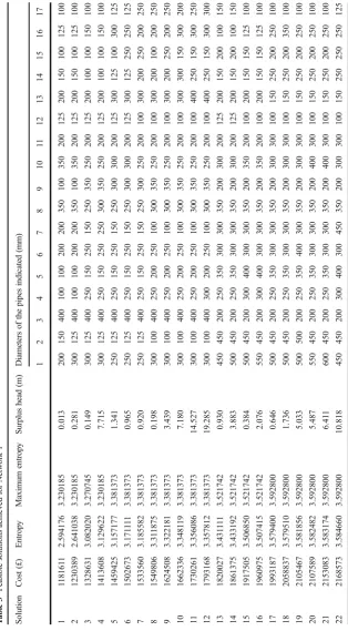
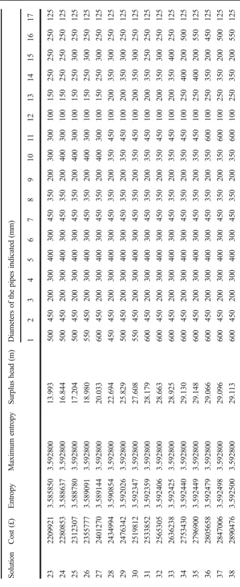
A typical sample of feasible solutions the proposed procedure yields is in theAppendix.

The sample has 38 feasible solutions. The correlationR2between entropy and hydraulic

reliability is 0.53. Between entropy and failure tolerance the correlation R2 is 0.13.

0 0.5 1 1.5 2 2.5 3 3.5

2.5 2.7 2.9 3.1 3.3 3.5 3.7

Entropy

0

1

£(

t

s

o

C

6)

Feasible Designs Infeasible Designs

(a)

(b)

2.5 2.7 2.9 3.1 3.3 3.5 3.7

0 20000 40000 60000 80000 100000

Total Deficit (m)

y

p

or

t

n

E

Feasible Designs

Infeasible Designs

2.5 2.7 2.9 3.1 3.3 3.5 3.7

3 3.1 3.2 3.3 3.4 3.5 3.6 3.7

Maximum Entropy

y

p

or

t

n

E

Feasible Designs

Infeasible Designs

(c)

(d)

0 0.5 1 1.5 2 2.5 3 3.5

0 20000 40000 60000 80000 100000

Total Deficit (m)

0

1

£(

t

s

o

C

6)

Feasible designs Infeasible designs

Fig. 2 Nondominated solutions achieved for Network 1 using two objectives.aTotal deficit in head vs. costb

However, it may be noted that the second objective function i.e. the hydraulic performance

deficitf2in Eq.7does not consider any surplus residual head. This is highly significant as

the surplus head is self-evidently a manifestation of redundancy. Therefore, a possible counter measure may entail screening out any solutions that are not Pareto-optimal based on the surplus head.

Accordingly, there are 14 solutions out of 38 that are nondominated based on the cost and

surplus head. For the 14 nondominated solutions the correlation R2 between entropy and

reliability is 0.95; and between entropy and failure toleranceR2is 0.80. Finally, as additional

validation, the solutions that are nondominated based on cost and reliability were identified. There are 11 solutions out of 38 that are nondominated based on the cost and reliability, with

entropy-reliability correlationR2of 0.93 and entropy-failure tolerance correlationR2of 0.74.

Only one solution out of 38 that is nondominated based on reliability and cost is not in the

cost-surplus head set of nondominated solutions (Solution 3 in Table1). This suggests the

procedure yields accurate and consistent results.

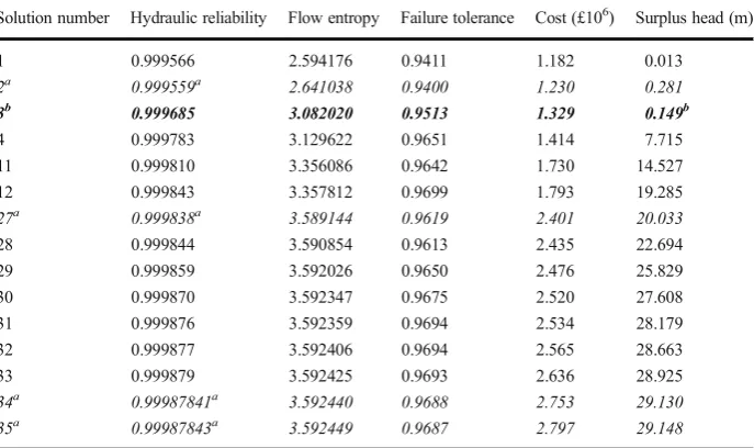
Table 1summarizes the nondominated solutions based on cost, hydraulic reliability and

surplus head. The reliability and failure tolerance analyses used the formulation in Tanyimboh

and Templeman (2000) and Tanyimboh and Sheahan (2002). The pipe failure simulations

applied head-driven analysis; the details are available in Tanyimboh et al. (2003) and

Tanyimboh and Templeman (2010). We used the Wagner et al. (1988) nodal head-flow

relationship to simulate conditions of subnormal pressure and the pipe failure model in

Cullinane et al. (1992).

Table 1 Nondominated solutions achieved for Network 1 based on cost vs. surplus head and/or cost vs.

reliability

Solution number Hydraulic reliability Flow entropy Failure tolerance Cost (£106_{) Surplus head (m)}

1 0.999566 2.594176 0.9411 1.182 0.013

2a _0.999559a _{2.641038 0.9400 1.230 0.281}

3b _{0.999685 3.082020 0.9513 1.329 0.149}b

4 0.999783 3.129622 0.9651 1.414 7.715

11 0.999810 3.356086 0.9642 1.730 14.527

12 0.999843 3.357812 0.9699 1.793 19.285

27a _0.999838a _{3.589144 0.9619 2.401 20.033}

28 0.999844 3.590854 0.9613 2.435 22.694

29 0.999859 3.592026 0.9650 2.476 25.829

30 0.999870 3.592347 0.9675 2.520 27.608

31 0.999876 3.592359 0.9694 2.534 28.179

32 0.999877 3.592406 0.9694 2.565 28.663

33 0.999879 3.592425 0.9693 2.636 28.925

34a 0.99987841a 3.592440 0.9688 2.753 29.130

35a 0.99987843a 3.592449 0.9687 2.797 29.148

a

5.2 Example 2

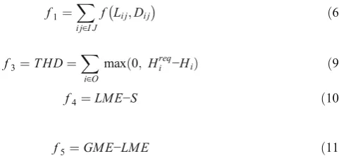
To assess the benefits of aggregating the hydraulic performance objectives, the optimization problem was also solved by considering the three hydraulic performance properties as separate objectives. Thus:

f1¼

X

i j∈I J

f Li j;Di j

ð6Þ

f₃¼T HD¼X i∈O

max 0ð ; Hreq_i −HiÞ ð9Þ

f₄¼LM E−S ð10Þ

f₅¼GM E−LM E ð11Þ

It may be recalled that f1 is the initial construction cost; f3=THD is the total head

deficit;f4is the amount by which the actual entropy of a solution is less than the maximum

entropy value achievable with the same flow directions; f5 is the amount by which the

maximum entropy value for the flow directions of the solution is less than the greatest of

the maximum entropy values. Each candidate solution is associated with anLME value

that is fixed and, obviously, there is only oneGMEwhose value is fixed also. Accordingly,

all the objectives, i.e.f1, f3, f4andf5, are minimized. Minimizingf4maximizesS.Similarly,

minimizingf5maximizesLMEby searching for alternative sets of flow directions that are

feasible and have larger LME values. For simplicity, for the purposes of the present

example, this formulation with separate hydraulic performance objectives is called Model

2 while the main formulation in Sections3and4, i.e. Equation8, is called Model 1.

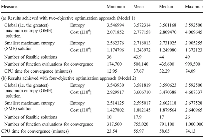
Table2compares the performance statistics for the two formulations with each set of

results based on 20 executions of the optimization algorithm. Some of the solutions in

Table 2 are not necessarily included in the final set of nondominated solutions in the

Appendix. The reason is that the Pareto-dominance in theAppendixis based on only the

costf1(Eq. 6) and hydraulic performance deficitf2(Eq. 7). For all optimization aspects

considered, it is self-evident that the approach of aggregating the objectives that measure the hydraulic performance of the water distribution system is superior. For example, for

the local and global maximization of entropy (i.e. the smallest maximum entropy, SME,

and global maximum entropy, GME, respectively) Model 1 that has two objectives

achieved significantly cheaper solutions with higher entropy values than Model 2 that has four objectives. This is attributable to the simplicity of assessing the trade-off between two objectives (entailing one pair-wise comparison) compared to four objectives (entailing six different pair-wise comparisons).

the optimization. Another particularly important result is that the aggregated performance objectives (Model 1) significantly improved the computational efficiency of the algorithm in terms of the

number of function evaluations and CPU time compared to Model 2 as Table2shows.

Furthermore, the Pareto-optimal front obtained by aggregating the performance objectives (Model 1) is so consistent that all solutions are non-dominated based on the total deficit in

nodal head and cost (Fig.2a). This may be because, for hydraulically infeasible solutions in

general, the entropy values are relatively small in comparison to the total deficit in nodal head. By contrast, most solutions obtained with separate performance objectives (Model 2) are

dominated based on the total deficit in nodal head and cost (Fig.3a). The number of feasible

solutions in the Pareto-optimal front is small and their distribution is uneven as can be seen in

Fig.3. Similarly, in the plots of entropy vs. cost and entropy vs. total deficit in head, the

relationships are quite clear for Model 1. By contrast, for Model 2, there are no clear patterns and, in fact, the majority the Pareto-optimal solutions are dominated based on entropy and cost and/or entropy and total nodal head deficit.

The motivation for maximizing entropy as part of the design optimization of a water distribution system is that, on its own, cost minimization leads inevitably to solutions that are inherently

unreliable due to the removal of redundancy in the cost minimization process (Templeman1982).

Thus the reason for including entropy in the optimization is to extend the range of feasible solutions achieved beyond the least-cost solution. Furthermore, the reason for maximizing the entropy both

locally (to find theLMEs) and globally (to find theGME) is to provide a diverse range of maximum

and/or near-maximum entropy solutions. Based on these goals, the graph of entropy vs. total deficit in head shows that the four-objective model is unsatisfactory; as the majority of the feasible

solutions found have the smallest entropy values (Fig.3b).

Recalling that every feasible set of flow directions corresponds to a maximum entropy

value, it can be expected that some of these sets of flow directions or LMEs may be

Table 2 Optimization statistics for network 1 based on 20 executions of the genetic algorithm

Measures Minimum Mean Median Maximum

(a) Results achieved with two-objective optimization approach (Model 1) Global (i.e. the greatest)

maximum entropy (GME) solution

Entropy 3.546994 3.572314 3.561168 3.592500

Cost (£106) 2.071852 2.777158 2.809470 4.009645

Smallest maximum entropy (SME) solution

Entropy 2.562376 2.718013 2.731925 2.905255

Cost (£106) 1.174796 1.243972 1.249080 1.372123

Number of feasible solutions 36 43.9 44 49

Number of function evaluations for convergence 174,700 508,140 435,600 999,500

CPU time for convergence (minutes) 12.95 37.67 32.29 74.09

(b) Results achieved with four-objective optimization approach (Model 2) Global (i.e. the greatest)

maximum entropy (GME) solution

Entropy 3.543930 3.581819 3.590623 3.592500

Cost (£106_{) 2.929917 3.606710 3.470388 4.607337}

Smallest maximum entropy (SME) solution

Entropy 2.514125 2.595017 2.602118 2.677528

Cost (£106) 1.427802 1.882145 1.879564 2.640965

Number of feasible solutions 10 17.9 17 26

Number of function evaluations for convergence 317,500 755,020 791,100 1,000,000

suboptimal compared to otherLMEsin their respective neighbourhoods in one or more respects. It is, therefore, very interesting that Model 1 with two objectives seems able to

select a generally superior and well distributed subset ofLMEvalues (Fig. 2d) whereas

Model 2 with four objectives seemingly cannot (Fig.3d). For example, the solutions in the

Pareto-optimal front for Model 1 belong to only 13 LME solution families or clusters

(Fig.2d). The solution families may be defined as two or more solutions derived from the

same feasible set of flow directions. These solutions can be expected to be generally similar and relatively close to one another in the solution space. The feasible solutions

achieved by Model 1 comprise eightLMEvalues out of 13. On the other hand, Model 2

provided considerably more LME values (Fig. 3d) of which only seven had feasible

solutions.

5.3 Example 3

Figure1bshows a network of a water distribution system in the city of Ferrara-I (Creaco et al.

2010,2012). The network has 49 nodes and 76 pipes; the total demand is 367 l/s; the head at

the two reservoirs is 30 m; the elevation of the demand nodes is zero; the total length of the

pipes is about 25.2 km; Manning’s roughness coefficient for the pipes is 0.015. The design

requirements for this network are that the residual head below which there is no flow is 5 m, while the residual head above which the demands are satisfied in full is 28 m. There are eight

pipe diameters in the range 150 to 500 mm. The solution space is thus 876= 4.314 × 1068.

Additional data including the pipe costs are available in Creaco et al. (2010,2012) and Saleh

0 0.5 1 1.5 2 2.5 3 3.5 4 4.5

0 20 40 60 80 100

Total Deficit (103 _m)

0

1

£(

t

s

o

C

6)

Infeasible solutions Feasible solutions

0 0.5 1 1.5 2 2.5 3 3.5 4 4.5

2.5 2.7 2.9 3.1 3.3 3.5 3.7

Entropy

0

1

£(

t

s

o

C

6)

Infeasible solutions Feasible solutions

(a)

(b)

2.5 2.7 2.9 3.1 3.3 3.5 3.7

0 20 40 60 80 100

Total Deficit (103 _m)

y

p

or

t

n

E

Infeasible solutions Feasible solutions

(c)

(d)

2.5 2.7 2.9 3.1 3.3 3.5 3.7

3 3.1 3.2 3.3 3.4 3.5 3.6 3.7

Maximum Entropy

y

p

or

t

n

E

Infeasible solutions Feasible solutions

Fig. 3 Nondominated solutions achieved for Network 1 using four objectives.aTotal deficit in head vs costb

(2013). A bit mutation rate of 1/228 or 0.004 was applied. Each solution comprises a chromosome of length 228 based on a 3-bit binary string per decision variable.

The solution space for this network is 1.944 × 1050times larger than Example 1. We kept

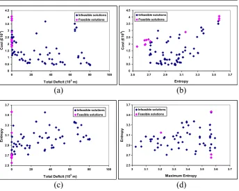
the population size (i.e. 100) and the maximum number of function evaluations allowed (i.e. one million) the same as in Example 1 to help illustrate the efficiency of the proposed simultaneous multi-directional search approach. The average CPU time for one million function evaluations was 42.08 min. The non-dominated solutions achieved include 27 feasible solutions. Additionally there are five marginally infeasible solutions. The shortfall in the residual head at the demand nodes is less than 1 cm in total, in three of the marginally infeasible solutions. For the other two marginally infeasible solutions the total shortfall in residual head is between 2 and 5 cm. Therefore, there are effectively 32 feasible solutions and 68 infeasible solutions in the final nondominated set. With only eight pipe sizes available, the proportion of feasible solutions achieved is quite reasonable as the required residual pressure of 28 m is stringent relative to the reservoir heads of 30 m.

The trade-off between cost and entropy can be seen in Fig.4b. The cheapest feasible solution

has cost and entropy values of €8.011 million and 4.7968 respectively, while the most

expensive one has cost and entropy values of€10.285 and 7.2989 respectively. The distribution

of feasible solutions over a wide range ofLMEvalues can be seen in Fig.4d. Indeed the feasible

6.5 7 7.5 8 8.5 9 9.5 10 10.5

0 1000 2000 3000 4000 5000

TD (m)

01

€

(t

so

C

6)

Feasible designs Infeasible designs

6.5 7 7.5 8 8.5 9 9.5 10 10.5

4 5 6 7 8

Entropy

01

€

(t

so

C

6)

Feasible designs Infeasible designs

(a)

(b)

4 4.5 5 5.5 6 6.5 7 7.5

0 1000 2000 3000 4000 5000

TD (m)

y

p

or

t

n

E

Feasible designs

Infeasible designs

4 4.5 5 5.5 6 6.5 7 7.5

4 5 6 7 8 9

ME

y

p

or

t

n

E

Feasible designs

Infeasible designs

(c)

(d)

Fig. 4 Nondominated solutions achieved for Network 2.aTotal deficit in head vs. costbEntropy vs. cost.c

solutions represent 26 differentLMEs, which provides further evidence of the effectiveness of the proposed approach for a multi-directional maximum-entropy search. Among the feasible solutions the largest surplus head at the critical node is 0.159 m. All the rest are small enough to suggest the solutions found are good or near optimal. The average value of surplus head, for the full set of 27 feasible solutions, is 0.035 m which is reasonable as the pipe sizes are discrete.

As mentioned in Example 1, the entropy values for some of the infeasible solutions seem questionable. This relates to the solutions in the lower branch of the graph of cost vs. entropy that has a negative gradient. This may be an anomaly due to demand-driven analysis. In other words, the entropy values in question may be based on pipe flow rates that, ordinarily, may not be achievable in practice. Also, in the graph of entropy vs. the total deficit in head, it can be seen that the entropy increases apparently as the deficit in head increases, up to a total deficit of about 3000 m. Additional investigations are therefore required to clarify this issue. These observations would appear to indicate that the performance of the proposed multi-directional search algorithm could be improved by replacing the demand-driven simulator with a

pressure-driven simulator (Seyoum and Tanyimboh2014; Gorev and Kodzhespirova2013; Kovalenko

et al.2014; Abdy Sayyed et al.2015).

6 Conclusions

The results of the proposed multi-directional search strategy in this article illustrate the effectiveness of maximizing the entropy values associated with different sets of flow directions while maintaining the objective of globally maximizing the entropy of the water distribution system and minimizing the cost. A good distribution of max-imum entropy values was achieved for the feasible designs. Clusters of feasible designs derived from different maximum entropy values were produced. In other words, multiple alternative optimal solutions are generated for each competitive set of flow directions that the procedure provides. Also, the application of the proposed concept of hydraulic performance deficit derived by combining the shortfall in entropy and the total node pressure deficit was successful in reducing the number of objec-tives and driving the evolutionary search. The new evolutionary search procedure was developed with a demand driven hydraulic simulator. Therefore, further investigation into the handling of pressure deficient solutions that may have misdirected the search is indicated. It appears that these complications could be avoided altogether by replacing the demand-driven hydraulic simulator with a head-driven simulator. Further research is thus indicated.

Acknowledgments This research was funded in part by the UK Engineering and Physical Sciences Research

Council (UK EPSRC Grant Reference EP/G055564/1) and the Government of Libya. Ananda Froes Alves (Science Without Borders exchange student from Federal University of Para, Brazil) contributed to this research by investigating the Pareto-dominance of solutions that have surplus residual pressure.

Compliance with Ethical Standards

Open AccessThis article is distributed under the terms of the Creative Commons Attribution 4.0 International License (http://creativecommons.org/licenses/by/4.0/), which permits unrestricted use, distribution, and repro-duction in any medium, provided you give appropriate credit to the original author(s) and the source, provide a link to the Creative Commons license, and indicate if changes were made.

References

Abdy Sayyed MAH, Gupta R, Tanyimboh TT (2015) Noniterative application of EPANET for pressure dependent modelling of water distribution systems. Water Resour Manag 29:3227–3242

Ang WK, Jowitt PW (2005a) Some new insights on informational entropy for water distribution networks. Eng Optim 37(3):277–289

Ang WK, Jowitt PW (2005b) Path entropy method for multiple-source water distribution networks. Eng Optim 37(7):705–715

Awumah K, Goulter IC, Bhatt SK (1990) Assessment of reliability in water distribution networks using entropy-based measures. Stoch Hydrol Hydraul 4(4):325–336

Awumah K, Goulter I, Bhatt SK (1991) Entropy based redundancy measures in water distribution networks. J Hydraul Eng 117(5):595–613

Baños R, Reca J, Martínez J, Gil C, Márquez AL (2011) Resilience indexes for water distribution network design: a performance analysis under demand uncertainty. Water Resour Manag 25:2351–2366

Burden RL, Faires JD (2001) Numerical analysis, Thomson learning. p 48–55

Creaco E, Franchini M, Alvisi S (2010) Optimal placement of isolation valves in water distribution systems based on valve cost and weighted average demand shortfall. Water Resour Manag 24(15):4317–4338 Creaco E, Franchini M, Alvisi S (2012) Evaluating water demand shortfalls in segment analysis. Water Resour

Manag 26(8):2301–2321

Cullinane MJ, Lansey KE, Mays LW (1992) Optimization-availability-based design of water distribution networks. J Hydraul Eng 118(3):420–441

Czajkowska AG, Tanyimboh TT (2013) Water distribution network optimization using maximum entropy and multiple loading patterns. Water Sci Technol Water Supply 13(5):1265–1271

Deb K, Pratap A, Agarwal S, Meyarivan T (2002) A fast and elitist multiobjective genetic algorithm: NSGA-II. IEEE Trans Evol Comput 6(2):182–197

Gheisi A, Naser G (2015) Multistate reliability of water-distribution systems: comparison of surrogate measures. J Water Resour Plan Manag. doi:10.1061/(ASCE)WR.1943-5452.0000529

Gorev NB, Kodzhespirova IF (2013) Noniterative implementation of pressure-dependent demands using the hydraulic analysis engine of EPANET 2. Water Resour Manag 27(10):3623–3630

Greco R, Di Nardo A, Santonastaso G (2012) Resilience and entropy as indices of robustness of water distribution networks. J Hydroinformatics 14(3):761–771

Herrera F, Lozano M, Verdegay JL (1998) Tackling real-coded genetic algorithms: operators and tools for behavioural analysis. Artif Intell Rev 12:265–319

Jayaram N, Srinivasan K (2008) Performance-based optimal design and rehabilitation of water distribution networks using life cycle costing. Water Resour Res 44:W01417

Kovalenko Y, Gorev NB, Kodzhespirova IF, Prokhorov E et al (2014) Convergence of a hydraulic solver with pressure-dependent demands. Water Resour Manag 28:1013–1031

Liu H, SavićDA, Kapelan Z, Zhao M, Yuan Y, Zhao H (2014) A diameter‐sensitive flow entropy method for reliability consideration in water distribution system design. Water Resour Res 50(7):5597–5610 Prasad TD, Park NS (2004) Multiobjective genetic algorithms for design of water distribution networks. J Water

Resour Plan Manag 130(1):73–82

Press WH, Teukolski SA, Vetterling WT, Flannery BP (2003) Numerical recipes in FORTRAN 77, vol. 1. Cambridge University Press, p 346–7

Raad DN, Sinske AN, van Vuuren JH (2010) Comparison of four reliability surrogate measures for water distribution systems design. Water Resour Res 46(5):W05524

Reca J, Martinez J, Banos R, Gil C (2008) Optimal design of gravity-fed looped water distribution networks considering the resilience index. J Water Resour Plan Manag 134(3):234–238

Rossman LA (2000) EPANET 2 users manual. U.S. Environmental Protection Agency, USA

Saleh SHA, Tanyimboh TT (2011) Global maximum entropy minimum cost design of water distribution systems. Proc. 13th water distribution systems analysis symposium,Palm Springs, California, USA, 206–213, 22–26 May 2011

Saleh SHA, Tanyimboh TT (2012) Joint pipe size and reliability design optimization of water distribution systems. Proc. 10th Int. Conference on Hydroinformatics, Hamburg, Germany, 14–18 July, 2012 Saleh SHA, Tanyimboh TT (2014) Optimal design of water distribution systems based on entropy and topology.

Water Resour Manag 28(11):3555–3575

Saleh S, Barlow E, Tanyimboh T (2012) Unbiased and accurate assessment of surrogate measures of hydraulic reliability of water distribution systems. 14th water distribution systems analysis conference, Adelaide Australia, ISBN 978-1-922197-58-9, p. 148–157, 24–27 September 2012

Saxena KS, Duro JA, Tiwari A, Deb K (2013) Objective reduction in many-objective optimization: linear and non-linear algorithms. Trans Evol Comput 17(1):77–99

Setiadi Y, Tanyimboh TT, Templeman AB (2005) Modelling errors, entropy and the reliability of water distribution systems. Adv Eng Softw 36(11–12):780–788

Seyoum AG, Tanyimboh TT (2014) Pressure dependent network water quality modeling. J Water Manage 167(6):342–355

Shannon C (1948) A mathematical theory of communication. Bell Syst Tech J 27(3):379–428

Siew C, Tanyimboh TT (2012a) Penalty-free feasibility boundary convergent multi-objective evolutionary algorithm for the optimization of water distribution systems. Water Resour Manag 26(15):4485–4507 Siew C, Tanyimboh TT (2012b) Pressure-dependent EPANET extension. Water Resour Manag 26(6):1477–1498 Tanyimboh T, Setiadi Y (2008) Joint layout, pipe size and hydraulic reliability optimization of water distribution

systems. Eng Optim 40(8):729–747

Tanyimboh T, Sheahan C (2002) A maximum entropy based approach to the layout optimization of water distribution systems. Civ Eng Environ Syst 19(3):223–225

Tanyimboh TT, Templeman AB (1993a) Calculating maximum entropy flows in networks. J Oper Res Soc 44(4): 383–396

Tanyimboh TT, Templeman AB (1993b) Optimum design of flexible water distribution networks. Civ Eng Syst 10(3):243–258

Tanyimboh TT, Templeman AB (1993c) Maximum entropy flows for single-source networks. Eng Optim 22(1): 49–63

Tanyimboh TT, Templeman AB (1993d) Using entropy in water distribution networks. In: Coulbeck B (ed.) Integrated computer applications in water supply, volume 1. Research Studies Press Ltd, Taunton, England, ISBN 086380 154 4, p. 77–90

Tanyimboh T, Templeman A (2000) A quantified assessment of the relationship between the reliability and entropy of water distribution systems. Eng Optim 33(2):179–199

Tanyimboh TT, Templeman AB (2010) Seamless pressure-deficient water distribution system model. J Water Manage 163(8):389–396. doi:10.1680/wama.900013

Tanyimboh TT, Tahar B, Templeman AB (2003) Pressure-driven modelling of water distribution systems. Water Sci Technol Water Supply 3(1–2):255–261

Tanyimboh TT, Tietavainen MT, Saleh SHA (2011) Reliability assessment of water distribution systems with statistical entropy and other surrogate measures. Water Sci Technol Water Supply 11(4):437–443 Templeman AB (1982) Discussion of optimization of looped water distribution systems, by GE Quindry, ED

Brill and JC Liebman. J Environ Eng 108(3):599–602

Todini E (2000) Looped water distribution networks design using a resilience index based heuristic approach. Urban Water 2(3):115–122

Vaabel J, Ainola L, Koppel T (2006) Hydraulic power analysis for determination of characteristics of a water distribution system. 8th annual water distribution systems analysis symposium, ASCE, Reston, VA, USA Wagner JM, Shamir U, Marks DH (1988) Water distribution reliability. J Water Resour Plan Manag 114(3):253–

294

Wu W, Maier HR, Simpson AR (2011) Surplus power factor as a resilience measure for assessing hydraulic reliability in water transmission system optimization. J Water Resour Plan Manag 137(6):542–546 Yassin-Kassab A, Templeman AB, Tanyimboh TT (1999) Calculating maximum entropy flows in multi-source,