A dynamic framework for managing the complexities of risks in megaprojects

1

A dynamic framework for managing the complexities of risks in megaprojects

*Boateng Prince

_{, Chen Zhen}

_{, Ogunlana O. Stephen}

1

_{Scott Sutherland School of Architecture and Built Environment, Robert Gordon University, Aberdeen, Scotland, UK}

_School

_{of Energy, Geoscience, Infrastructure and Society, Heriot-Watt University, Edinburgh, Scotland, UK}

*[email protected]

Abstract

The future of mega infrastructure projects is certain - there will be more risks to manage! The challenge is being met through research and innovation combining current approaches with new. This research adopted a dynamic approach through the combination of Analytical Network Process (ANP) and system dynamics (SD) as an innovative methodology known as SDANP to model complexity in megaprojects design and construction. We communicate how the SDANP model could explore problems caused by Social, Technical, Economic, Environmental and Political (STEEP) risks to construction cost, time and performance and provide insights that lead to organizational learning. We proceed to exemplify by means of a real-life case project in the City of Edinburgh and offer suggestions on what front-ended stakeholders could do to improve the management of risks in megaprojects. The results of the application showed that, when compared to traditional risks assessment methods, this SD model with integrated ANP revealed improvements in managing risks according to STEEP risks criteria. The new framework appears to be a superior solution for solving the dynamic complexities of risks during megaproject design and construction. The findings of the study contribute to the project management theoretical development within the field of megaproject management.

Keywords: Analytical Network Process, megaprojects, risk complexity, system dynamics.

1.Introduction

This study presents a heuristics approach in prioritising and assessing risk complexity in megaproject construction and then tests the model on a transportation construction project. The model incorporates both tangibles like work-to-do, project cost and intangibles such as uncertainties, grievances, and inadequate project complexity analysis in the risk assessment process by using the Analytical Network Process (ANP) to prioritise risks and the system dynamics (SD) approach to simulate the dynamics of such risks overtime within the SDANP framework to increase the analytical and the dynamic capabilities of traditional risk assessment methods. Most construction risk assessment models include analytical parameters such as cost, duration, quality, probabilities, etc., without incorporating heuristics. With regards to the increasingly complex and dynamics of megaprojects coupled with new procurements methods, the tendency today is to use risk quantification and modelling more as vehicles to

promote effective risk response planning amongst multi-disciplinary project team members. (Davies et al. 2014) emphasised that, an effective risk management approach can provide a framework to identify and assess potential risks so that response actions can be taken to mitigate them. However, many of the risk management approaches developed by contractors and their consultants are not dynamically enough to analyse and assess risk (Too and Too, 2010). As a result, communicating construction project risks become poor, incomplete, and inconsistent throughout the construction supply chain.

2 factors from the ANP were then modelled within SDANP framework to appraise their measured impact on the cost, time and quality performance of the project. The approach is to gain a fuller understanding of the interrelationships between the multiple variables in the system. Also, it is to demonstrate the potential benefits of the SDANP approach. The aim of the paper therefore, is to explore and model using the SDANP framework, problems caused by STEEP risks to construction cost, time and performance and provide insights that lead to organizational learning. The knowledge gain could be used to improve the accuracy of risks estimation, thereby reducing the problem of cost and time overruns during megaproject delivery. The objectives of this research are to:

 develop a framework that incorporates Social, Technical, Economic, Environmental and Political (STEEP) risks into a SDANP methodology for risks assessment in megaproject during construction and

 test the SDANP methodology on a transportation megaproject

For researchers, the findings would contribute to the project management theoretical development within the field of megaproject management. It will further provide an innovative framework that offers a platform to incorporate tangible and intangible risk variables into a risk assessing process using ANP for prioritising risks and SD for simulating those risks overtime. For practitioners, it challenges the paradigm of considering the new methodology as a successful risk assessment in megaprojects. When compared to traditional risks assessment methods, the results obtained from the integration of the ANP and SD methodology revealed improvements in managing risks according to STEEP risks criteria. The new framework appears to be a superior solution for solving the dynamic complexities of risks during megaproject design and construction.

1.1. Literature Review

The literature review is segmented in two main categories. This includes: (a) overview of the Analytical Network Process and (b) Current trend of SD applications in construction project management. 1.1.1.The Analytical Network Process (ANP)

The ANP is a methodological tool developed by Thomas Saaty. The tool is leveraged for this research because of its significance in multi-criteria decision

making (MCDM) when an extensive number of factors are involved. The ANP is a more general form of the Analytic hierarchical Process (AHP) for ranking alternatives based on some set of criteria.

Unlike AHP, ANP is capable of handling feedbacks and interdependencies, which exist, in complex systems like the STEEP risks system in megaproject development. ANP problem formulation starts by modelling the problem that depicts the dependence and influences of the factors involved to the goal or higher-level performance objective. The ANP as a methodology has a precise language regarding the components of the problem and the relationship between them. In Saaty (2005), the ANP was defined as a systematic approach which uses both the quantitative and qualitative factors for multiple criteria decisions. As a decision making tool, the ANP is made up of a network of criteria and alternatives (which are all called elements), grouped into clusters. These elements in the network can be related in any possible way to incorporate feedback and interdependent relationships within and between clusters. This provides a more natural approach for modelling complex environment, such that a more objective concept which leads to the most influential to the goals will be obtained. That is, in the context of this study, ANP offers a high flexibility for modelling and prioritizing risk. ANP can break down more clearly the risk attributes, not limited to the probabilities, but also all possible potential consequences, in more specific criteria.

3 and detailed literature review (Sipahi and Timor 2010, Lombardi et al. 2011)

1.1.2. Current Trend of SD Application in Construction

The System Dynamic (SD) is a field developed by Jay Forrester in mid 1950s. It is a methodology used for modelling and analysing the behaviour of complex social systems in an industrial context (Sterman 2000). It was designed to help decision-makers learn about the structure and dynamics of complex systems. It is used to design high leverage policies for sustained improvement, and to catalyse successful implementation and change. SD has been used by researchers and project managers in many fields to understand various social, economic and environmental systems in a holistic view (Towill 1993, Rodrigues and Bowers 1996, Sycamore and Collofello 1999, Love et al. 2002, Mawby and Stupples 2002, Ogunlana et al. 2003, Williams et al. 2003). Sterman (1992) and Lyneis and Ford (2007) demonstrated SD capabilities in improving construction project management. Saeed and Brooke (1996) used SD to model how civil engineering

contracts can be improved through dynamic reasoning. Love et al., (2000) developed SD model to model design errors and rework in construction projects. Ogunlana et al., (2003) used SD to explore performance enhancement in a construction organisation. Park et al. (2004) offered a dynamic model for construction innovation. Nasirzadeh et al (2008) used SD to assess the impact of different risks on construction project objectives. Boateng et al. (2012) used SD to model the impacts of critical weather conditions on construction activities and further describe the approach of SD in assessing risks in megaproject during construction (Boateng et al. 2013).

2. Methodology

2.1. SDANP Framework

4

Model verification

 Expert opinion

Model development

 Develop formulae for flow diagrams

Initial model development

Model simulation

Model validation

Testing of model structure & behaviour

Policy analysis, design and improvement and implementation

Test not passed

 Reference modes

 Model boundary chart

 Feedback structure

 Casual flow diagram

Model Testing

 Dimensional consistency

 Structure consistency

Test passed

Test not passed

Test passed Software application

Develop and structure the ANP model

List of Top n

“priority risks”

w

w

R

n

j

ij





i wi

Normalized criteria

Perform Risk Priority Index (RPI) Calculation

R

W

RPI



List of potential risks

Database

Risks identification and categorization

Perform Mean Scores of importance

      



i

E

n MV

1 ( ,,)

1  Literature on STEEP

 Case studies

Data source

 Data from source documents of past similar projects

ANP route SD route

1 ... ... 1 .... 1 ... ... ... ... 1 1 1 21 1 12 R R R R R R R R n n ij ji ij n   PRw

Conduct pairwise Comparison

Conduct prioritization survey based on experts’ decisions

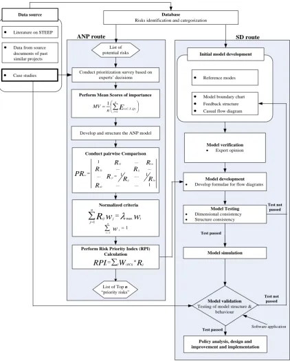
Fig. 1: The Proposed SDANP Framework for risk assessment (Boateng 2014)

Data Source: - This is the source from which data for project risks originate. The sources include the literature, documents of past and similar projects and case studies.

The database: - This is the channel used to categorize identified risks within the organization and to store information about projects. The information stored here is used to facilitate the data transfer into both the ANP and the SD.

5 given their specific subjectivity inputs. The experts’ decisions are the preset choices made by the experts based on the the risk prioritization survey for selecting potentially “high risks” using a Likert type scale of 1 to 5 to score the level of STEEP risks impact on megaproject objectives (cost, time and quality) in the construction phase. A weighted quantitative score (WQS) method is used to translate experts’ decisions during prioritization surveys into synthetize numerical values to derive the mean scores of importance. The mean scores can be significantly distinguished based on participant’s experience, background and as well as information in regard to a case study project by using Equation 1.

MV =1

n(∑ Ei(C,T,Q) n

i=1 ) (1)

Where

- MV indicates the value of mean scores of importance for each criteria/sub-criteria calculated by WQS.

- E refers to the experimental WQS for each sub/criteria expressed as a percentage year of experience multiplied by each participant’s score of importance.

- icis the participant’s score of importance for

each sub/criteria with respect to cost. - it is the participant’s score of importance for

each sub/criteria with respect to time. - iqis the participant’s score of importance for

each sub/criteria with respect to quality. - nis the total number of participants in this

research.

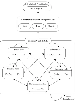
Decisions made at the point of risk synthetisation can be subjected to adjustment due to changing priorities. Following the calculation of the mean score, the ANP models can then be developed based on experts’ decisions into criteria, sub-criteria and options as indicted in figure 2.

The ANP Network Model for Risk Prioritization illustrate in Figure 2 consists of three clusters: ‘Goal’, ‘Criterion’ and ‘Option.’ Cluster ‘Goal’ contains only one element as the statement of the purpose for risk prioritization within which the category of ‘High risks’ are listed according to the results from the pairwise comparison calculation. Cluster ‘Criterion’

6

Option: Potential Risks

Inner dependencies

SV1,Sv2…………..Svn

ENv1………..ENvn

TV1,TV2,……... TVn,

Social risks

PV1,PV2,………... PVn, EV1,EV2, ………EVn,

Technical risks

Political risks Economic risks

Environmental risks List of high risks

Goal: Risk Prioritization

Criterion: Potential Consequences on:

Cost Time Quality

Fig. 2: ANP Network Model for Risk Prioritization (Boateng 2014)

Table 1

Relative importance and data transformation inpairwise comparison

Intensity of

importance Definition (Saaty 1996) Data transformation mechanism(Chen et al. 2011)

1 Equal 1:1

2 Equally to moderately dominant 2:1, 3:2, 4:3, 5:4, 6:5, 7:6, 8:7, 9:8 3 Moderately dominant 3:1, 4:2, 5:3, 6:4, 7:5, 8:6, 9:7 4 Moderately to strongly dominant 4:1, 5:2, 6:3, 7:4, 8:5, 9:6

5 Strongly dominant 5:1, 6:2, 7:3, 8:4, 9:5

6 Strongly to very strongly dominant 6:1, 7:2, 8:3, 9:4

7 Very strongly dominant 7:1, 8:2, 9:3

8 Very strongly to extremely dominant 8:1, 9:2

9 Extremely dominant 9:1

7 Using Equation (2), the comparison matrix for each cluster can be performed. Let W = {Wj | j = 1, 2 ... n} be the set of criteria. The result of the pairwise comparison on n criteria can be summarized in an (n x n) evaluation matrix PR in which every element Rij (i, j = 1, 2... n) is the quotient of weights of the criteria. This pairwise comparison can be shown by a reciprocal matrix. That is, if activity i has one of the above non-zero numbers assigned to it when compared with activity j, then j has the reciprocal value when compared with i. The results of the comparisons are represented by dimensionless quotients to measure the preference of one option over the other. A direct numerical appreciation is not required from the decision maker, but rather a relative appreciation. PR is the potential risks and Rij, the comparison between risk variables i and j.

𝑃𝑅 = (𝑅𝑖𝑗)_{𝑛𝑥𝑛|} | 1 1 𝑅12 ⁄ ⋮ 𝑅12 1 𝑅_{𝑗𝑖=1 𝑅}

𝑖𝑗 ⁄ … 𝑅𝑖𝑗 ⋱ 𝑅1𝑛 𝑅2𝑛 ⋮ 1 𝑅1𝑛

⁄ 1 _𝑅

2𝑛

⁄ … 1

| |

(2) (2)

Once the pairwise comparison is completed for the whole network, the vector corresponding to the maximum eigenvalue of the constructed matrices is computed and a priority vector is obtained. The priority value of the concerned element is established by normalizing this vector as described in equation 3. ∑nj=1Rijwi= λmaxwi (3) Where ‘R’ is the matrix of pairwise comparison, ‘w’ is the eigenvector, and ‘λmax’ is the maximum eigenvalue of [R]

By substitution, the maximum eigenvalue (λmax) is

calculated to derive a new matrix (W). The matrix (W) is then used to multiply comparison matrix (R) with (wi) as indicates in Equation 4. Finally, the (λmax)

can be obtained by averaging the values obtained from Equation 4. Computations of the process used to calculate the maximum eigenvalue (λmax) is shown

in Equation (5).

| | 1 1 𝑅12 ⁄ ⋮ 𝑅12 1 1 𝑅23 ⁄ … 𝑅23 ⋱ 𝑅1𝑛 𝑅2𝑛 ⋮ 1 𝑅1𝑛

⁄ 1 _𝑅

2𝑛

⁄ … 1

| |_{x |}

𝑤1 𝑤2 ⋮ 𝑤𝑛 | = | 𝑊1 𝑊2 ⋮ 𝑊𝑛

| (4)

𝜆𝑚𝑎𝑥 = 1 𝑛 (

𝑊1

𝑤1+

𝑊2

𝑤2+ … … +

𝑊𝑛

𝑤𝑛) (5)

During the risk assessment process, a problem may occur in the consistency of the pairwise comparisons. The consistency ratio is used to check the consistency of the calculation and to provide a numerical assessment of the process. If the calculated ratio is less than 0.10, consistency is considered to be satisfactory. The conceptual model is then imported into a Super Decision Software to perform the pairwise comparison. The aim of constructing pairwise matrices is to derive the relative weight of each potential risk. Finally, the risk prioritization index (RPI) is calculated using equation 6 to support final decision making. The criterion to make this selection is the weights of alternatives that can be taken from a synthesised super-matrix derived from the Super Decision Software. Although the RPI can be performed manually with the equation 6, it was performed by the Super Decisions Software in this study. Computation priorities command was used to determine the priorities of all the nodes in the network

𝑅𝑃𝐼𝑖= ∑ 𝑊𝑖 (𝐶,𝑇,𝑄)∗ 𝑅𝑖𝑗 (6) Where ‘RPIj’represents the global priority of the risk

options i, ‘Wj,’ the weight of the criterion j with

respect to project cost, time and quality, and ‘Rij’, the

local priority

After the priority computation, the RPIs can be classified into five states of likelihood and consequence on project cost, time and quality so that a five-by five matrices can be against each risk as either “very high”, “high”, “moderate”, “low” or “very low”. The risk prioritization index (RPI) calculation is the platform where the analytical framework is combined with the experts’ decisions to produce independent assessments on project priorities without further input from the experts. Finally, the results obtained from the RPI calculation can be listed as the ‘n’ priority risks for further decision making.

8

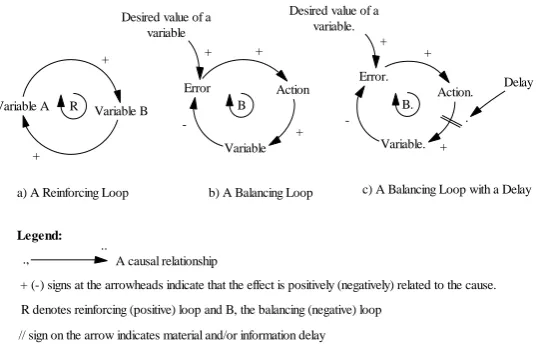
Fig. 3: The Three Components of System Dynamics Models.

SD can be used to model systems in both qualitative and quantitative manner. SD models can be constructed from three basic building blocks: positive feedback or reinforcing loops, negative feedback or balancing loops, and delays. Positive loops (called reinforcing loops) are self-reinforcing while negative loops (called balancing loops) tend to counteract change. Delays in SD models indicate potential instability in the system. Figure 3a shows how a reinforcing loop feeds on itself to produce a growth in a system to correspond to positive feedback loops in control theory. For example, in Figure 3a, an increase in variable (A) leads to an increase in variable (B) (as indicated by the “+” sign) and that in turn leads to additional increase in variable (A) and so on. The “+” sign indicates on the head of the arrow does not necessarily mean that the values produced in the system will increase. It is just that variable (A) and variable (B) will change in the same direction of polarity. If variable (A) decreases, then variable (B) will decrease. In the absence of external influences, both variable (A) and variable (B) will clearly grow or decline exponentially. Reinforcing loops generate growth, amplify deviations, and reinforce change. A balancing loop indicated in Figure 3b is a structure that changes the current value of a system variable or a desired or reference variable through some action. It corresponds to a negative feedback loop in control theory. A (-) sign indicates that the values of the variables change in opposite directions. The difference between the current value and the desired

value is perceived as an error. An action proportional to the error is taken to decrease the error so that, over time, the current value approaches the desired value. The third basic element is a delay, which is used to model the time that elapses between cause and effect. A delay is indicated by a double line, as shown in Figure 3c. Delays make it difficult to link cause and effect (dynamic complexity) and may result in unstable system behaviour. Based on a verified Causal Loop Diagram, a stock and flow diagram indicated in figure 4 can be developed using the ‘n’ priority risks derived from the ANP computation and the inputs which the experts provided to facilitate in-depth stock and flow modelling and risk simulation overtime.

The governing equations used to calculate the entire system parameters can also be formulated at this point. To understand accumulation process of inflow of uncertainties, it is important to know the mathematical meaning used to integrate the flow of risk influences into the system. Based on a mathematical definition of the integral, the level of risk impacts inside a stock will be the integration of total flows of uncertainties on the stock (See equation 7).

Stock (t)= ∫ [flowstotal t

0 (s)]ds (7)

Where ∫ [flowstotal t

0 (s) is a function of the total flow in the system.

Variable A _{Variable B} +

+

Desired value of a variable

Error Action

Variable

+ +

+

-Desired value of a variable.

Error.

Action.

Variable. +

+

+

-R B B.

Delay

.

a) A Reinforcing Loop b) A Balancing Loop c) A Balancing Loop with a Delay

.,

..

A causal relationship

Legend:

+ (-) signs at the arrowheads indicate that the effect is positively (negatively) related to the cause.

R denotes reinforcing (positive) loop and B, the balancing (negative) loop

9

Fig. 4: A simple Stock and Flow Model

Inflow (Uncertainty) indicates the increasing amount of risk level in the stock (Risk accumulation container). In the other hand, outflow (certainty) decreases the level of risk impacts in the stock. Using ANP’s RPI as the quantity of risk impact level in the stock at the initial time, the equation above becomes the following:

Stock (t)= ∫ [flowstotal t

0 (s) − Outflow(s)]ds +

Stock(0) (8)

Where 𝑆𝑡𝑜𝑐𝑘(0) is the stock of risk impact level (RPI) at the initial time, (t = 0).

In Systems Dynamics, verbal descriptions and causal loop diagrams are more qualitative; stock and flow diagrams and as well as model equations are more of quantitative ways to describe a dynamic situation. Since Systems Dynamics is largely based on the soft systems thinking, (learning paradigm), it is well suited to be applied on those managerial problems which are ambiguous and require better conceptualization and insight (Madachy 2007).

2.2.Test of the SDANP for Dynamic Risk Management

The proposed SDANP methodology was subjected to a case study to measure its effectiveness in performing dynamic risk assessment in megaproject construction.The case study project is ETN project. It consisted initially of three lines and was designed to run through the City Centre of Edinburgh. The construction involved new bridges, retaining walls, viaducts, the tram depot and control centre, electrical sub stations to provide power to the overhead lines at 750 volts, track laying and tram stops. The initial contract value was £545 million, with a contract period of 3 years. The project was procured using a

turnkey contract. The client (City of Edinburgh Council aka CEC) used a private limited company known as Transport Initiatives Edinburgh (TIE) to deliver the tram system. Until August 2011, ETN project was overseen by TIE (a company wholly owned by CEC) and was responsible for project-managing the construction of the tramway. Further role of TIE was to administer, integrate and coordinate the consultants and principal contractor (a consortium of Bilfinger Berger and Siemens) involved in the project. By February 2011, contractual disputes and further utility diversion works resulted in significant delays to the project beyond the originally planned programme. In late 2011, TIE was released from managing the ETN Project. Turner and Townsend (T&T), a project management consultant was brought in by CEC to ensure effective oversight and delivery of the project. Work in 2012 continued smoothly on schedule with a new governance structure under the management of T&T until the project was completed in summer 2014.

3.Results and Discussion

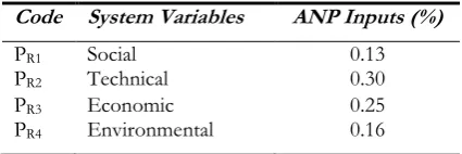
In SDANP simulation, trend analysis is given priority and numbers do not have much significance, however, the numbers should be, as far as possible, close to the real life situations. In the context of the STEEP risks modelling, the ANP input to the system to conduct simulation is represented in Table 2.

Table 2

Summary of the ANP Inputs

Code System Variables ANP Inputs (%)

PR1 Social 0.13

PR2 Technical 0.30

PR3 Economic 0.25

PR4 Environmental 0.16

Also, the outputs indicated on Table 3 revealed the

dynamic simulation results underthe following time

bounds and units of measurements for system variables:

PR1:Social risks Social

uncertainty. +

Social Certainty

-Initial level for RP1 = RPI for PR1

. ..

A causal relationship Legend:

+ (-) signs at the arrowheads indicate that the effect is positively (negatively) related to the cause.` ,

RP denotes Potential Risk and RPI, Risk Priority Index ....

Flow

10 i. The initial time for the simulation = 2008, Units: Year ii. The final time for the simulation= 2015, Units: Year iii. The time step for the simulation = 0.125, Units: Year iv. Unit of measurement for system variables =

Dimensionless

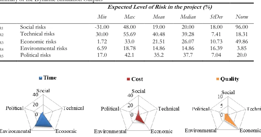
It can be observed on Table 3 and Figure 5 that project time and cost are all impacted by STEEP risks. The mean impact levels of all risks in

succession from PR1 to PR5 on ETN project is

revealed to be 19%, 40.48%, 21.50%, 14.86% and 35.20%. Time was the most sensitive to the impact of economic, environmental and political risks whilst cost was sensitive to the impact of the economic, environmental, political and social risks. On the other hand, project quality was sensitive to the economic, environmental and political risks.

Table 3

Summary of the Dynamic Simulation Outputs

Expected Level of Risk in the project (%)

Min Max Mean Median StDev Norm

PR1 Social risks -31.00 48.00 19.00 20.00 18.00 96.00

PR2 Technical risks 30.00 55.69 40.48 39.28 7.41 18.31

PR3 Economic risks 1.72 33.0 21.51 26.07 10.73 49.86

PR4 Environmental risks 6.59 18.78 14.86 14.86 16.39 3.85

PR5 Political risks 17.0 42.1 35.2 37.7 7.04 20.0

Fig. 5: Measured Impact of STEEP Risks

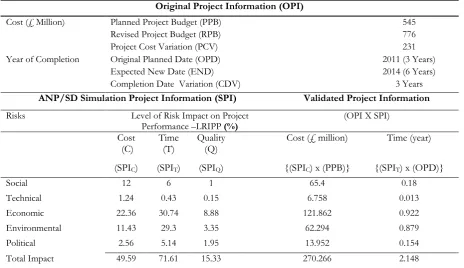
3.1 SDANP Model Validation

For practical reasons, empirical tests were conducted to examine the ability of the STEEP model to match the historical data of the case study project. Information gathered from the real system was compared to the simulated results. As Table 4 indicates, the total level of risks impacted on the ETN project which resulted to cost and time overruns and project quality deficiency is 49.53% on cost, 71.61% on time and 15.33% quality. Prior to the dynamic simulation, the planned budget for the project was £545 million and was expected to be completed in 3 year. Later, the planned budget of the project was revised to £776 million and that of the planned completion time to 6 years. After simulation was performed, the result was validated against the real system to reveal the actual STEEP risks implication on the project performance. The validation results revealed that the actual project cost

11

Table 4

Data Validity on Edinburgh Tram Network Project

Original Project Information (OPI)

Cost (£ Million) Planned Project Budget (PPB) 545

Revised Project Budget (RPB) 776

Project Cost Variation (PCV) 231

Year of Completion Original Planned Date (OPD) 2011 (3 Years)

Expected New Date (END) 2014 (6 Years)

Completion Date Variation (CDV) 3 Years

ANP/SD Simulation Project Information (SPI) Validated Project Information

Risks Level of Risk Impact on Project

Performance –LRIPP (%) (OPI X SPI)

Cost

(C) Time (T) Quality (Q) Cost (£ million) Time (year) (SPIC) (SPIT) (SPIQ) {(SPIC) x (PPB)} {(SPIT) x (OPD)}

Social 12 6 1 65.4 0.18

Technical 1.24 0.43 0.15 6.758 0.013

Economic 22.36 30.74 8.88 121.862 0.922

Environmental 11.43 29.3 3.35 62.294 0.879

Political 2.56 5.14 1.95 13.952 0.154

Total Impact 49.59 71.61 15.33 270.266 2.148

Boateng (2014)

The simulation results further revealed that the quality of ETN project was impacted by 15.33%. However, there was no available historical data on the original level of project quality deficiency to be validated against with this output. Hence, the hypothesized system which was initially made up by expert’s knowledge was used to compare the real system. This was the case so that a better presentation of the real system with the model system can be experimented to achieve a higher degree of confidence in the SDANP model. Examples of expert knowledge calibration techniques used are meetings with academic staff, some members of European Cooperation in Science and Technology (E-COST) in charge of scientific research in megaproject effective delivery, industrial stakeholders and as well as the use of the ANP application.

4. Conclusions

To reduce risks, front-end stakeholders involve in megaproject development can use the new generic tool for risk management in five steps: risk management planning, risk identification, qualitative and quantitative risk analysis, risk response planning, risk monitoring and control.

Step 1: Risk management planning- Within the STEEP risk management planning, feedback loops concerning project risks can be used by planners to pro-actively test and improve the existing project plan such as forecasting and diagnosing the likely outcomes of the current plan.

Step 2: Risk identification-The SDANP models can support risk identification in a qualitative level through the causal loop diagrams. Given STEEP as specific risks, it is possible to identify which feedback loops favour or counter the occurrences of such risks so that the direct or indirect impacts of the project magnitude can be understood.

12 full impacts of the risks occurrences and impacts on megaprojects during construction.

Step 4: Risk response planning- The models can be effectively used to support risk response planning in megaproject development in three ways.

- Provide a feedback perspective for risk identification

- Provide a better understanding of the multiple- factor causes of risks and a trace through the chain to identify further causes and effects.

- Serve as powerful tools to support project managers to devise effective responses.

Step 5: Risk monitoring and control- The models provide effective tools for risk monitoring and control. Through the cause and effects diagrams, early signs of unperceived risk emergence can be identified to avoid aggravation. In addition, simulated models can provide an effective monitoring and control mechanism for risk diagnosis.

Based on the above reasons, it would therefore be more appropriate to assess risks in megaprojects during construction with the SDANP framework so that every project management team member at the decision level can benefit from the knowledge that went into making these decisions before arriving at the final level of risk implications on the megaproject objectives throughout the project schedule time. The goal of the SDANP risk assessment approach is not to eliminate all risks from the project. Rather, it is to recognize the significant risk challenges and the complexities of those challenges on the project performance overtime so that an appropriate management responses can be initiated to mitigate those challenges.

References

Azadnia, A. H. , Saman, M. Z. M. and Wong, K. Y. (2015). Sustainable supplier selection and order lot-sizing: An integrated multi-objective decision-making process. International Journal of Production Research, 53(2), 383-408.

Boateng, P. (2014). A dynamic systems approach to risk assessment in megaprojects, Royal Academy of Engineering Centre of Excellence in Sustainable Building Design, School of the Built Environment, Heriot-Watt University, UK. Boateng, P., Chen, Z. and Ogunlana, S. (2012). A

conceptual system dynamic model to describe the impacts of critical weather conditions in megaproject construction. Journal of Construction Project Management and Innovation, 2(1), 208-24.

Boateng, P., Chen, Z., Ogunlana, S. and Ikediashi, D. (2013). A system dynamics approach to risks description in megaprojects development. Organization, Technology & Management in Construction: An International Journal, 4(Special Issue), 0-.

Chen, Z., Li, H., Ren, H., Xu, Q. and Hong, J. (2011). A total environmental risk assessment model for international hub airports. International Journal of Project Management, 29(7), 856-66.

Davies, A., MacAulay, S., DeBarro, T. and Thurston, M. (2014). Making innovation happen in a megaproject: London's crossrail suburban railway system. Project Management Journal, 45(6), 25-37.

Ergu, D., Kou, G., Shi, Y. and Shi, Y. (2014). Analytic network process in risk assessment and decision analysis. Computers & Operations Research, 42(0), 58-74.

Eshtehardian, E., Ghodousi, P. and Bejanpour, A. (2013). Using anp and ahp for the supplier selection in the construction and civil engineering companies; case study of iranian company. KSCE Journal of Civil Engineering, 17(2), 262-70.

Kumar, G. and Maiti, J. (2012). Modeling risk based maintenance using fuzzy analytic network process. Expert Systems with Applications, 39(11), 9946-54.

Lee, S., Geum, Y., Lee, S. and Park, Y. (2015). Evaluating new concepts of pss based on the customer value: Application of anp and niche theory. Expert Systems with Applications, 42(9), 4556-66.

Liang, S. and Wey, W. (2013) Resource allocation and uncertainty in transportation infrastructure planning: A study of highway improvement program in taiwan. Habitat International, 39(0), 128-36.

Lombardi, P., Giordano, S., Farouh, H. and Yousef, W. (2011) An analytic network model for smart cities. In, Proceedings of the International Symposium on Analytic Hierarchy Process, 1-6.

Love, P. E., Mandal, P., Smith, J. and Li, H. (2000). Modelling the dynamics of design error induced rework in construction. Construction Management & Economics, 18(5), 567-74.

13 Lyneis, J. M. and Ford, D. N. (2007). System

dynamics applied to project management: A survey, assessment, and directions for future research. System Dynamics Review, 23(2‐3), 157-89.

Madachy, R. J. (2007). Software process dynamics. John Wiley & Sons.

Mawby, D. and Stupples, D. (2002). Systems thinking for managing projects. In, Engineering Management Conference, 2002. IEMC '02. 2002 IEEE International, 2002, Vol. 1, 344-9 vol.1.

Nasirzadeh, F., Afshar, A., Khanzadi, M. and Howick, S. (2008). Integrating system dynamics and fuzzy logic modelling for construction risk management. Construction Management and Economics, 26(11), 1197-212.

Ogunlana, S. O., Li, H. and Sukhera, F. (2003). System dynamics approach to exploring performance enhancement in a construction organization. Journal of Construction Engineering and Management, 129(5), 528-36.

Park, M a P-M, F. (2004) Reliability buffering for construction projects. Journal of Construction Engineering and Management, 130(5), 626-37. Pourjavad, E. and Shirouyehzad, H. (2014).

Evaluating manufacturing systems by fuzzy anp: A case study. International Journal of Applied Management Science, 6(1), 65-83.

Rodrigues, A. and Bowers, J. (1996). The role of system dynamics in project management. International Journal of Project Management, 14(4), 213-20.

Saaty, T. L. (1996). Decision making with dependence and feedback: The analytic network process. Vol. 4922, RWS publications Pittsburgh.

Saaty, T. L. (2005). Theory and applications of the analytic network process: Decision making with benefits, opportunities, costs, and risks. Pittsburgh. Pennsylvania: RWS Publications. Saeed, K. and Brooke, K. (1996). Contract design for

profitability in macro‐engineering projects. System Dynamics Review, 12(3), 235-46.

Shen, K-Y. and Tzeng, G-H. (2014). A decision rule-based soft computing model for supporting financial performance improvement of the banking industry. Soft Computing, 1-16.

Sipahi, S. and Timor, M. (2010). The analytic hierarchy process and analytic network process: An overview of applications. Management Decision, 48(5), 775-808.

Sterman, J. D. (1992). System dynamics modeling for project management. Unpublished manuscript, Cambridge, MA.

Sterman, J. D. (2000) Business dynamics: Systems thinking and modeling for a complex world. Chicago, IL: Irwin/McGraw Hill.

Sycamore, D. and Collofello, J. S. (1999). Using system dynamics modeling to manage projects. In, Computer Software and Applications Conference, 1999. COMPSAC '99. Proceedings. The Twenty-Third Annual International, 1999, 213-7.

Tjader, Y., May, J .H., Shang, J., Vargas, L. G. and Gao, N. (2014). Firm-level outsourcing decision making: A balanced scorecard-based analytic network process model. International Journal of Production Economics, 147, Part C(0), 614-23. Too, E. and Too, L. (2010). Strategic infrastructure

asset management: A conceptual framework to identify capabilities. Journal of Corporate Real Estate, 12(3), 196-208.

Towill, D. R. (1993). System dynamics- background, methodology and applications. 1. Background and methodology. Computing & Control Engineering Journal, 4(5), 201-8.

Williams, T., Ackermann, F. and Eden, C. (2003). Structuring a delay and disruption claim: An application of cause-mapping and system dynamics. European Journal of Operational Research,

148(1), 192-204.

Yeh, T-M. and Huang, Y-L. (2014). Factors in determining wind farm location: Integrating gqm, fuzzy dematel, and anp. Renewable Energy,