A Low Complexity SI Sequence Estimator For Pilot-Aided
SLM-OFDM Systems
Saheed A. Adegbite∗, Scott G. McMeekin, Brian G. Stewart
School of Engineering and Built Environment, Glasgow Caledonian University, G4 0BA, Glasgow, UK
Abstract
Selected mapping (SLM) is a well-known method for reducing peak-to-average power
ra-tio (PAPR) in orthogonal frequency division multiplexing (OFDM) systems. However, as
a consequence of implementing SLM, OFDM receivers often require estimation of some
side information (SI) in order to achieve successful data recovery. Existing SI estimation
schemes have very high computational complexities that put additional constraints on
lim-ited resources and increase system complexity. To address this problem, an alternative
SLM approach that facilitates estimation of SI in the form of phase detection is presented.
Simulations show that this modified SLM approach produces similar PAPR reduction
per-formance when compared to conventional SLM. With no amplifier distortion and in the
presence of non-linear power amplifier distortion, the proposed SI estimation approach
achieves similar data recovery performance as both standard SLM-OFDM (with perfect
SI estimation) and also when SI estimation is implemented through the use of an existing
frequency-domain correlation (FDC) decision metric. In addition, the proposed method
significantly reduces computational complexity compared with the FDC scheme and an
ML estimation scheme.
Keywords: OFDM, PAPR reduction, selected mapping, side-information detection
∗Corresponding author, Tel: +44 141 273 1225
1. Introduction
O
rthogonal frequency division multiplexing (OFDM) is now the preferred layer-1 tech-nology in various high speed communication system standards including 4G-Long Term Evolution (4G-LTE) because it offers high spectral efficiency, immunity to multipathfading and provides a means to achieve very high data rate transmission. These are all
attractive attributes of any high speed communication system [1, 2]. However, OFDM has
a characteristic high peak-to-average power ratio (PAPR) [2–4], which may increase power
consumption, degrade system performance and put additional constraints on the design
and implementation of Power Amplifiers (PAs), Digital-to-Analogue (D/A) and
Analogue-to-Digital (A/D) converters [3]. In addition, high PAPR signal levels often drive a PA to
operate in its non-linear region, causing signal distortion in the form of increased
bit-error-rate (BER). In theory, non-linear PA distortion can be avoided using a PA with a large
linear region i.e. large input back off (IBO). Unfortunately, this approach is difficult to
achieve in practice and it often results in poor PA efficiency, which reduces battery life span
of mobile terminals and increases design costs [4, 5]. Therefore, for practical purposes, low
PAPR signals are desirable in OFDM systems.
An in-depth review of various PAPR reduction techniques has been presented in [6].
Amongst these, is the selected mapping (SLM) scheme. SLM [7] is a well established
method for reducing PAPR in OFDM. SLM creates alternative copies of the same OFDM
signal by using a number of phase rotation sequences to modify phases of individual OFDM
subcarriers within the original OFDM signal, then selecting and transmitting the
time-domain signal that has the lowest PAPR value. Unfortunately, SLM introduces additional
constraints in that it requires transmission and detection of some side information (SI),
which contains vital information on how the transmitted OFDM signal was constructed
at the transmitter. The transmission of SI reduces data throughput and the need for SI
detection increases the receiver’s computational requirements.
mission are discussed in [8] and [9]. Assuming all possible SLM phase rotation sequence
vectors are known at the receiver, SI estimation is achieved in [8] using pilot-assisted
Maximum Likelihood (PAML) and in [9] based on frequency-domain correlation (FDC)
decision metrics. However, computational complexities associated with these schemes are
high and are proportional to the number of alternative SLM phase rotation sequence
vec-tors, U. These are unattractive when a larger value of U is used to improve the PAPR
reduction performance. Also, since these pilot-assisted SI estimation schemes require the
re-construction or storage of allU phase rotation sequence vectors at the receiver, there is
a considerable level of system overhead associated with the implementation of both PAML
and FDC SI estimation schemes.
To further reduce the computational complexity associated with SI estimation in
pilot-assisted SLM-OFDM systems, this paper presents a pilot-pilot-assisted SI estimation method,
which requires no SI transmission at the transmitter and no reconstruction of all candidate
SLM phase rotation sequences at the receiver. The proposed method is also based on an
extension of the work carried out in [10]. The proposed scheme in this paper differs from
the work studied in [10] in that it uses a different SI estimation criterion based on a hard
decision rule while the method in [10] applied a Maximum Likelihood (ML) detection
cri-terion. For comparisons with the proposed method, the FDC based SI estimation scheme,
presented in [9] is selected because it is based on the use of conventional SLM sequences
and also gives slightly improved PAPR reduction performance over [8]. Simulations show
that the modified SLM presented in this paper produces nearly similar PAPR reduction
performance as conventional SLM. In addition, the proposed method achieves similar data
recovery performance compared with existing SI estimation scheme presented in [9] and
also when perfect knowledge of SI was assumed, with and without the presence of non-linear
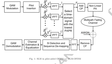
Fig. 1: SLM in pilot-aided OFDM i.e. SLM-OFDM
2. Conventional SLM-OFDM System and FDC Scheme
This section gives an overview of the conventional SLM method of reducing PAPR and
SI estimation based on the FDC scheme studied in [9]. Fig. 1 shows a block diagram
representation of a pilot-assisted SLM-OFDM system.
Conventional Pilot-assisted SLM-OFDM
Consider a pilot-aided OFDM symbol blockX of lengthNv, which consists ofNp pilot Xp, and Nd data Xd symbols. For 0 ≤ k ≤ Nv−1 where k is a subarrier index, each
subcarrier symbol denoted byX[k] inX is mapped to a subcarrier index kthrough
X[k] =X[mL+l], 0≤m≤Np−1
= ⎧ ⎪ ⎨ ⎪ ⎩
Xp[mL], l= 0
Xd[mL+l], otherwise
whereNv =Nd+Np,Lrepresents the pilot spacing i.e. the number of subcarriers between
two successive pilot symbols, land m are arbitrary indices.
Using phase rotation sequence vectors denoted byBufor 0≤u≤U−1,U alternative OFDM signals are constructed through SLM. One of the modified OFDM signals, denoted
by xu¯, will have the lowest PAPR value. Thus, the selected and transmitted signalxu¯ is therefore given by
xu¯ =IF F T{Bu¯·X}
= √1
N
Nv−1
k=0
Bu¯[k]·X[k]exp(−j2πnk/N) (2)
where 0≤n≤N−1.
The value of ¯uis obtained from
¯
u= arg min
u∈0,1, ... U−1
max{|xu|2}
E{|xu|2} , wherex
u=IF F T{Bu·X} (3)
whereE{·}is the expectation function for evaluating the mean power of signal xu. The value of ¯umust be known at the receiver in order to achieve successful data
recov-ery since it contains the critical information on howxu¯ was formed. The value of ¯uorBu¯ is commonly referred to as SI.
After transmission over a fading channel with frequency response H, the received OFDM symbolY¯ can be expressed as
¯
Y =HXu¯+V, whereXu¯ =X·Bu¯ (4)
where V represents complex-valued additive white Gaussian noise (AWGN) sequences. Similar toX in (1), data components ofY¯,H and V can be denoted by Y¯d,Hd and Vd
respectively and their pilot components as Y¯p, Hp and Vp respectively. Since the SI is
FDC SI Estimation
Let ˆu represent an estimate of the SI. Using the FDC based SI estimation studied in
[9], ˆu is obtained from
ˆ
u= arg max
u ∈ 0,1, ... U−1Re{R
u} (5)
whereRu is the FDC function, defined by
Ru = 1
Np−1 Np−1
m=1
ˆ
Hu
p[m]·Hˆpu[m−1]∗, (6)
and
ˆ
Hu p[m] =
¯
Yp[m]Bpu[m]∗
Xp[m]
(7)
where∗ represents a complex conjugate operator.
In terms of computational complexity based on number of complex multiplications
(CMs) and additions (CAs), the calculation of the FDC function Ru in (6) requires
U(Np−1) CMs and U(Np−2) CAs while the computation of ˆHpu[m] in (7) requires UNp
CMs. In total, the FDC based SI estimation scheme requiresU(2Np−1) CMs andU(Np−2)
CAs. It can be noted that these evaluations assume that Bpu[m]∈ ±1. In addition, since
most implementations will involve real-valued operations, each complex-valued operation
i.e. CMs and CAs are re-expressed in terms of real multiplications (RMs) and additions
(RAs). From the definition in [9],
1 CM4 RM + 2 RA and 1 CA2 RA. (8)
Thus, the FDC scheme will require an estimated total number of 4(2UNp−U) RMs and
6U(Np−1) RAs.
Using the estimated SI value ˆu, SLM de-mapping is performed to remove the applied
an SLM de-mapping procedure, which gives
Y[k] = ¯Y[k]Buˆ[k]∗. (9)
Similarly, using the value of ˆu, the pilot sub-channel estimate ˆHp[m] is obtained from
ˆ
Hu p[m] as
ˆ
Hp[m] = ˆHpuˆ[m]. (10)
The next stage of data decoding involves finding an estimate of the received subcarrier
symbol from
ˆ
Xd[k] = min D[q]∈Q
Y
d[k]−Hˆd[k]D[q]
2
(11)
whereQis the set ofQconstellation pointsD[q] of the chosen data modulation scheme for
0≤q≤Q−1, ˆXd[k]∈Qis the estimated data symbol, and ˆHd[k] is an estimate of data
sub-channel, obtained by linear interpolation between values of ˆHp[m].
3. Proposed Method
An alternative SI estimation method based on a binary phase detection approach is
now proposed in an attempt to reduce the SI estimation computational complexity when
compared with the methods in [9] and [10]. The proposed SI estimation method in this
paper uses similar modified SLM method, which is referred to as clustered SLM (C-SLM),
and is described in [10]. However, the proposed SI estimation is different compared with
the approach in [10].
Similar to [10], the proposed method involves partitioning of OFDM symbol block X intoNp/2 consecutive clusters, each having two consecutive pilot symbols andW −2 data
symbols whereW = 2L.
Fig. 2 shows a block diagram representation of the considered clustering. For 0≤c <
(Np/2)−1, the cluster form of X[k] can be represented by
Xc[w] =X[cW+w] =X[k], 0≤w≤W −1
= ⎧ ⎪ ⎪ ⎪ ⎪ ⎪ ⎨ ⎪ ⎪ ⎪ ⎪ ⎪ ⎩
Xc[we] =Xp[cW +we], we= 0, we∈w
Xc[wo] =Xp[cW +wo], wo=L, wo∈w
Xc[wd] =Xd[cW+wd], otherwise
(12)
where wd = 1, 2 . . . L−1, L+ 1 . . . W −1, we and wo represents w indices for every
first and second pilot symbol in each cluster respectively. Henceforth, the first and second
pilots in each cluster will be referred to as the ‘even-indexed pilot’ and ‘odd-indexed pilot’
respectively.
Similar to SLM, the C-SLM method produces alternative copies of the original OFDM
symbol, then selects and transmits the one that has the lowest PAPR value. In contrast to
SLM, which performs phase rotation on each of the subcarrier symbols (data and pilots)
with different phase values, C-SLM phase rotates all data subcarrier symbol and the
odd-index pilot in each cluster with a common phase value while the even-odd-index pilot remains
LetJu represent C-SLM phase rotation sequences whereJu ∈ ±1, elements ofJuare defined as
Ju
c[w] =Ju[cW +w] =Ju[k]
= ⎧ ⎪ ⎨ ⎪ ⎩ Ju
c[we] = 1
Ju
c[wo] =Jcu[wd] =Jcu =±1.
(13)
Thus, application ofJu toX produces Xu as expressed through
Xu
c[w] =Xu[cW +w] =Xu[k]
= ⎧ ⎪ ⎪ ⎪ ⎪ ⎪ ⎨ ⎪ ⎪ ⎪ ⎪ ⎪ ⎩ Xu
c[we] =Xc[we]
Xu
c[wo] =Xc[wo]Jcu
Xu
c[wd] =Xc[wd]Jcu.
(14)
The lowest PAPR signalxu¯, obtained through C-SLM is given by
xu¯ n=
1 √
N
Nv−1
k=0
Xu¯[k]ej2πnkN , 0≤n≤N −1 (15)
whereXu¯ =X·Ju¯ and Ju¯ =ejαu¯ denotes the optimum C-SLM sequence vector.
At the receiver, letZ represent the received OFDM sequences whereZis expressed by
Thus, each of the received subcarrier (in clustered form)Zc[w] is represented by
Zc[w] =Hc[w]Xc[w]Jcu¯+Vc[w],
= ⎧ ⎪ ⎪ ⎪ ⎪ ⎪ ⎨ ⎪ ⎪ ⎪ ⎪ ⎪ ⎩
Hc[we]Xc[we] +Vc[we], w=we,
Hc[wo]Xc[wo]Jcu¯+Vc[wo], w=wo,
Hc[wd]Xc[wd]Jcu¯+Vc[wd], w=wd.
(17)
Unlike the FDC based SI estimation method previously described in (5), an estimate of
the SI termJcu¯can also be achieved from the odd-indexed pilot sinceJcu¯[wd] =Jcu¯[wo] =Jcu¯
[10].
First, an odd-indexed ¯Hc[wo] and an even-indexed ˆHc[we] terms are computed from
ˆ
Hc[we] = Zc
[we]
Xc[we]
= Hc[we]Xc[we] +Vc[we]
Xc[we]
=Hc[we] + V c[we]
Xc[we]
(18a)
¯
Hc[wo] = Zc
[wo]
Xc[wo]
= Hc[wo]Xc[wo]J ¯
u
c +Vc[wo]
Xc[wo]
=Hc[wo]Jcu¯+
Vc[wo]
Xc[wo].
(18b)
At high signal-to-noise ratio (SNR) where the effects of the additive noise terms are
negli-gible, a simplified expression for ¯Hc[wo] becomes
¯
Hc[wo]≈Hc[wo]Jcu¯ (19)
ˆ
Hc[we] has no associated phase rotation value (sinceJcu¯[we] = 1, see (13)) while ¯Hc[wo] has
an associated phase rotation termJc¯u. Therefore, ˆHc[we] represent the even-indexed pilot
sub-channel estimate while ¯Hc[wo] represent an odd-indexed channel term.
It can be seen from the expression in (19) that an estimate of the SI term Jcu¯ can be
obtained from ¯Hc[wo]. However, since ¯Hc[wo] has an associated channel termHc[wo], some
form of channel cancellation is required to mitigate the channel fading effects. To achieve
this, a ‘normalised’ (with respect to ˆHc[we]) complex-valued term Rc is first obtained
through
Rc = ¯Hc[wo]
ˆ
Hc[we]
= Hc
[wo]Jcu¯+ Vc[wo] Xc[wo]
Hc[we] +XVcc[[wwee]]
. (20)
By omitting the additive noise terms for simplicity,Rc can be re-expressed as
Rc ≈ Hc
[wo]Jcu¯
Hc[we] .
(21)
By letting ¯αc represent the phase component of Rc, a polar coordinate representation of
Rc is given as
Rc=|Rc|exp(jα¯c). (22)
From the expression in (21), it can be noted that by assuming a slow channel fading
condition whereHc[wo]≈Hc[we], an estimate ˆJc of the applied C-SLM sequence value Jcu¯
can be calculated fromRc.
The method in [10]
For each c index, let ˆJc denotes the estimate of Jcu¯ where ˆJc ∈ ±1. Using the ML
estimation approach described in [10], the SI estimate ˆJc is computed from
ˆ
Jc = min λi∈±1
exp(jα¯
c)−λi
2
whereλi is an arbitrary variable used to determine whether ˆJc is +1 or−1 [10]. It can be
seen that the implementation of (23) requires a total of Np | · |2 operations andNp CAs.
However, the need for several|·|2computations can increase the computational complexity
of the method in [10].
An alternative SI estimation method is now proposed in an attempt to further reduce
the computational complexity of computing ˆJc. The proposed method is based on a hard
decision criterion and is now described.
Proposed: Hard Decision Estimation
Since Jcu¯ ∈ ±1, then its estimate ˆJc ∈ ±1. Let ˆJc = exp(jαˆc) where the value of ˆαc is
either 0 orπ. Unlike the ML method, ˆJc is indirectly determined from an estimate of the
phase term ˆαc.
In the proposed method, an estimate of the phase term ˆαc is calculated from a hard
decision criterion given by
ˆ
αc =
⎧ ⎪ ⎨ ⎪ ⎩
0, if|α¯c| ≤π/2
π, otherwise
(24)
where ¯αc is the phase component of Rc as previously defined in (22). Note that since ¯αc is
a real-valued number, then the computational complexity of obtaining an absolute value
of ¯αc in (24) is negligible and is ignored.
From the expressions in (23) and (24), it can be noted that both methods (ML scheme
and the proposed method) differ in their estimation of ˆJc. It can also be seen that both
methods require the computation of ˆHc[we] in (18a), ¯Hc[wo] in (18b), Rc in(20) and ¯αc
from Rc. The phase ¯αc of a complex-valued variable (like Rc) can be evaluated through
the use of the well-known Taylors series expansion described in [11, ch. 16]. It is estimated
that using the Taylors expansion, 5Np RMs and 2Np RAs are required to evaluate the
Table 1: Computational complexity of computing ˆHc[we], ¯Hc[wo], ¯αc, andRc
Variables Computational Complexity
ˆ
Hc[we] in (18a) Np/2 CMs≡2Np RMs +Np RAs
¯
Hc[wo] in (18b) Np/2 CMs≡2Np RMs +Np RAs
Rc in (20) Np/2 CMs≡2Np RMs +Np RAs
¯
αc from Rc 5Np RMs + 2Np RAs
of computing ˆHc[we], ¯Hc[wo], ¯αc and Rc. As before, these evaluations (in Table 1) are
re-expressed in terms of RAs and RMs computations using (8). Using the Taylors expansion
method, computing the magnitude | · |of a complex-valued number requires 19 RMs and
8 RAs (see Appendix). Hence, computingNp | · |2 operations in (23) requires 20Np RMs
+ 8Np RAs. Note that an additional RM operation is required to compute| · |2 compared
with| · |. Hence, the combined computational complexity of computing ˆHc[we], ¯Hc[wo], ¯αc
and Rc is 11Np RMs + 5Np RAs.
Using ˆJc, data sub-channel estimates ˆHc[wd] are obtained by linear interpolation
be-tween values of ˆHc[we] and ˆHc[wo] where
ˆ
Hc[wo] = ¯Hc[wo] ˆJc∗. (25)
ˆ
Yc[wd] = Zc
[wd]
¯
Hc[wo]
×Hˆc[wo]
ˆ
Hc[wd]
= Hc[wd]Xc[wd]J ¯
u c
Hc[wo]Jcu¯
×Hˆc[wo]
ˆ
Hc[wd]
= Hc[wd]Xc[wd]
Hc[wo] ×
ˆ
Hc[wo]
ˆ
Hc[wd]
. (26)
In a similar to (11), the final data decoding stage determines an estimate of the nearest
constellation point to ˆYc[wd].
6.5 7 7.5 8 8.5 9 9.5 10 10.5 11 11.5 12 10−4
10−3 10−2 10−1 100
γ
(dB)
CCDF(
γ
) = Pr ( PAPR >
γ
)
original OFDM Conventional SLM Proposed: C−SLM
[image:14.612.88.505.220.599.2]U = 2
U = 8
4. Simulation Results and Comparisons of Computational Complexity
This section presents comparisons of computational complexity of considered methods
and discusses the Matlab simulation results on PAPR reduction and BER performance.
4.1. Simulation Results
With values of [Np and L] set to [100 and 6] respectively, simulations consider OFDM
transmission over three different channel models namely: (1) the extended pedestrian
chan-nel (EPA), defined in [12]; (2) 6-tap COST-207 rural-area chanchan-nel (RA6), defined in [13]
and (3) the 3GPP rural-area channel (3gppRA), defined in [14]. As defined for LTE
sys-tems, pilots are obtained from Gold codes sequences, OFDM subcarrier spacing is 15 KHz,
guard interval is 5.21 μs and sampling frequency is set to 15.36 MHz (when N = 1024
and Nv = 600). Data symbols are obtained using a 64-QAM modulation scheme. SLM is
performed using chaotic-binary sequences studied in [15] and PAPR reduction performance
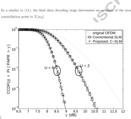
is measured by evaluating the well known complementary cumulative distribution function
(CCDF). The CCDF gives the probability that a calculated PAPR of an OFDM signal
exceeds a certain threshold denoted byγ. Thus, the CCDF ofγ is defined as
CCDF{γ}=P rob(P AP R≥γ). (27)
Fig. 3 shows comparisons of CCDF curves of the OFDM signal before PAPR reduction
(labelled as ‘original OFDM’), with PAPR reduction using conventional SLM and the
pro-posed C-SLM method for U set to 2 and 8. Results in Fig. 3 show that the proposed
method produces nearly similar PAPR reduction performance as conventional SLM for
each value ofU.
using the IBO parameter. The IBO of a PA is defined as
IBO (dB) = 10 log10
Psat
Pavg
(28)
where Psat and Pavg respectively denote PA input saturation power and mean power of
the input signal. In this paper, the amplitude modulation (AM) effects of PA is modelled
using the well known Rapp’s model [16]. Simulations consider a solid state PA (SSPA),
commonly used in mobile communications systems [17]. The output AM/AM conversion
of a SSPA, with unity gain, is described by Rapp’s model through
y(t) = x(t) 1 +
|x(t)|
Asat
2ρ1/2ρ (29)
where x(t) represents the input signal into the SSPA, y(t) is the output signal from the
SSPA,Asat is the SSPA output saturation magnitude andρis the smoothing factor which
controls the PA’s transition from linear to saturation region i.e. the higher the value of
ρ, the sharper the transition from linear to non-linear operating region of the SSPA. For
accurate modelling of an SSPA,ρ is set to 3 [18, ch. 2].
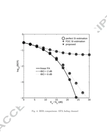
The data recovery performance of the proposed method is compared with that of a
standard SLM-OFDM (when perfect SI knowledge is assumed) and with SI estimation
based on the FDC scheme for IBO values: ∞dB, 2 dB, and 6 dB. Note that the case when
IBO =∞dB represent an SLM-OFDM system with no non-linear PA distortion i.e. linear
PA.
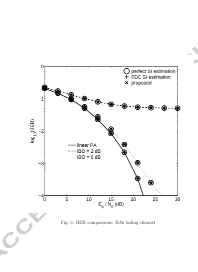
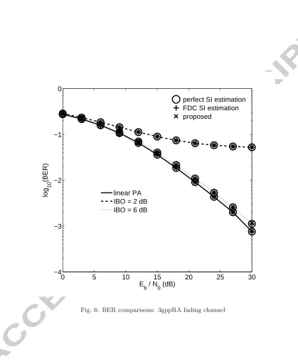
Figs. 4 to 6 compare BER curves between the proposed method, standard SLM-OFDM
(which assumes perfect SI estimation) and the FDC method over EPA, RA6 and 3gppRA
0 5 10 15 20 25 30
−4 −3 −2 −1 0
E
b / N0 (dB)
log
10
(BER)
perfect SI estimation FDC SI estimation proposed
[image:17.612.83.517.86.649.2]linear PA IBO = 2 dB IBO = 6 dB
0 5 10 15 20 25 30
−4 −3 −2 −1 0
E
b / N0 (dB)
log
10
(BER)
perfect SI estimation FDC SI estimation proposed
[image:18.612.90.486.92.635.2]linear PA IBO = 2 dB IBO = 6 dB
0 5 10 15 20 25 30
−4 −3 −2 −1 0
E
b / N0 (dB)
log
10
(BER)
perfect SI estimation FDC SI estimation proposed
[image:19.612.91.510.100.612.2]linear PA IBO = 2 dB IBO = 6 dB
environments and IBO levels, the proposed method produces the same BER performance
as both the FDC based SI estimation scheme and standard SLM-OFDM, which assumes
perfect knowledge of SI. This is partly because of the inherent phase cancellation (SLM
de-mapping) within the proposed method, and also because of the slow fading channel
conditions.
It can be noted the BER performance of the ML estimation method described in [10]
is not presented to avoid duplicity of previous results in [10]. The key advantage of the
proposed method over the FDC based SI estimation scheme and the ML method is now
demonstrated through the comparison of their computational complexity.
4.2. Computational Complexity
From the previous descriptions in Table 1, Table 2 shows summary of the computational
requirements of computing expressions in (23) and (24) for the ML estimation method in
[10] and the proposed method respectively. From Table 2, it can be seen that the proposed
scheme requires a total of 11Np RM and 5Np RA computations while the ML estimation
method in [10] requires 31Np RMs and 15Np RAs. Note that these evaluations ignores
the complexity of real-valued compare operations because it is negligible relative to the
complexity of RMs and RAs. Table 3 shows comparisons of the number of RM and RA
op-erations required by the FDC, the ML estimation method in [10] and the proposed method.
It can be noted (in Table 3) that the computational complexity of both the proposed
method and the method in [10] is independent of the value of U. In addition, unlike the
FDC scheme, both the ML estimation approach and the proposed method require no
knowl-edge of all candidate SLM sequences during data decoding. Therefore, it is expected that
the proposed method has a significant computational advantage (over the FDC scheme) as
the value ofU is increased.
Using Table 3, the computational complexity advantage of the proposed method is
numerically evaluated using the well known Computational Complexity Reduction Ratio
Table 2: Computation requirements of the ML estimation method in [10] and the proposed SI estimation
method
ML method [10] Proposed
ˆ
Jc is directly computed from (23)
ˆ
Jcis computed as exp(jαˆc) where ˆαc
is derived from (24)
Complexity of computing ˆHc[we], ¯Hc[wo],
¯
αc and Rc is 11Np RMs + 5Np RAs
Same as the ML method.
The expression in (23) requiresNp|·|2and
Np CAs. Note that Np CAs ≡ 2Np RAs
and each|·|2 requires 20NpRMs plus 8Np
RAs.
To compute ˆαc, Np/2 real-valued
compare operations are required.
and RMs). The CCRR is defined as [9]
Table 3: Comparisons of computational complexity in terms of RMs and RAs
Computational Complexity FDC Method in [10] Proposed
RMs 4(2UNp−U) 31Np 11Np
RAs 6U(Np−1) 15Np 5Np
CCRR =
1− complexity of the proposed method complexity of other scheme
×100%. (30)
The CCRR value represents the amount (expressed as a %) of reduction in computational
complexity offered by the proposed method relative to either the FDC scheme or the ML
approach [19]. Table 4 shows comparisons of estimated CCRR values for RMs and RAs
whenU is set to: 4, 8 and 16. High CCRR values for the proposed method as highlighted
in Table 4 suggest that the proposed method requires significantly reduced computational
complexity compared with the existing FDC scheme in [9] and the ML method in [10].
As expected, it can be seen that the computational complexity of the ML approach is
independent on the value ofU.
5. Conclusions
An alternative SI estimation technique is proposed for an SLM-OFDM receiver. The
proposed method used a modified SLM scheme known as C-SLM to reduce PAPR and
performed SI estimation through the use of a hard binary decision rule. In terms of PAPR
reduction, the C-SLM method offered nearly similar PAPR reduction capability to
Table 4: CCRR of the proposed method relative to both the FDC scheme and the ML method
Parameters Operations FDC scheme ML method
U = 4
RM 77% 64%
RA 84% 66%
U = 8
RM 88% 64%
RA 92% 66%
U = 16
RM 94% 64%
RA 96% 66%
estimates without the knowledge of all possible phase rotation sequences and produced
sim-ilar data recovery performance to both standard SLM-OFDM (with perfect knowledge of
SI) and the FDC based SI estimation scheme. The proposed method is an attractive choice
over other methods because it required significantly reduced computational complexity.
Appendix
Computing Amplitude and Phase of a Complex Number
For a complex number C, let |C|and θ respectively be the magnitude and phase ofC.
The real and imaginary components ofC is respectively represented byCre andCim. Then,
from Euler’s formula, the complex numberC is given by
C=Cre±jCim=|C|exp(±jθ)
=|C|cos(θ)±j|C|sin(θ). (31)
GivenC,θcan be computed from
θ= tan−1
Cim
Cre
From the expression in (31), the magnitude|C|is obtained as
|C|=Cre
cos(θ) OR |C|=Cim
sin(θ). (33)
Using numerical computational methods, the arctangent function tan−1(x) in (32) is
com-puted using Taylor series expansion described in [20]
tan−1(x) =x−x 3
3 +
x5 5 −
x7 7 +
x9
9 − . . . (34)
Note thatx is a real-valued number. Using a Matlab tool called taylortool, it was verified
that the first 5 terms in a Taylor series approximation is sufficient to produce identical
results as that from actual Matlab implementation of trigonometric functions.
Computational Complexity of Computing θ=tan−1(x)
To compute tan−1(x) using the expression in (34), the x2 term is first computed so as
to enable the subsequent computation ofx3,x5,x7 andx9 terms.
The computation ofx2 requires 1 real multiplication (RM), and the computation ofx3,
x5,x7 and x9 each require 1 RM according to the following:
x3 =x2·x; x5=x3·x2
x7 =x5·x2; x9=x7·x2 (35)
Here, it is assumed that the computation of, for example,x7 will use the results from the
initial computation ofx5 and the pre-computed x2. Similarly, the computation of x9 will
use initial results ofx7 and x2.
The four divisions and additions in (34) require equivalent of 4 RMs and 4 real additions
(RAs). Hence, a total number of 9 RMs and 4 RAs are required to compute tan−1(x).
Therefore, to compute the phase of a complex number, 10 RMs and 4 RAs operations are
Computational Complexity of Computing θ
= 10 RMs plus 4 RAs
Computational Complexity of Computing |C|
From the expression in (33), the cosine function cos(θ) can also be derived using the
Taylor series expansion [20]
cos(θ) = 1−θ 2
2! +
θ4 4! −
θ6 6! +
θ8
8! − . . . (36)
Note that θ is also a real-valued number and the evaluations in (36) assume that the
factorial of a number is pre-computed and known. Similar to the arctan function, the
first 5 terms of Taylor series implementation of a cosine function is found to give a good
approximation.
In a similar manner to tan−1(x), computing cos(θ) also requires 8 RMs and 4 RAs.
Hence, to compute the magnitude|C|of a complex number, a total number of 19 RMs and
8 RAs is required. Note that the additional RM is from the division operation in (33).
Computational Complexity of Computing |C|
= 19 RMs plus 8 RAs
References
[1] S. Adegbite, B. G. Stewart, S. G. McMeekin, Least Squares Interpolation Methods for
LTE System Channel Estimation over Extended ITU Channels, International Journal
[2] N. I. Miridakis, D. D. Vergados, A Survey on the Successive Interference Cancellation
Performance for Single-Antenna and Multiple-Antenna OFDM Systems,
Communica-tions Surveys Tutorials, IEEE 15 (1) (2013) 312–335.
[3] T. Jiang, Y. Wu, An Overview: Peak-to-Average Power Ratio Reduction Techniques
for OFDM Signals, Broadcasting, IEEE Transactions on 54 (2) (2008) 257–268.
[4] X. Li, L. J. Cimini, Effects of clipping and filtering on the performance of OFDM,
Communications Letters, IEEE 2 (5) (1998) 131–133.
[5] G. Santella, F. Mazzenga, A hybrid analytical-simulation procedure for performance
evaluation in M-QAM-OFDM schemes in presence of nonlinear distortions, Vehicular
Technology, IEEE Transactions on 47 (1) (1998) 142–151.
[6] Y. Rahmatallah, S. Mohan, Peak-To-Average Power Ratio Reduction in OFDM
Sys-tems: A Survey And Taxonomy, Communications Surveys Tutorials, IEEE 15 (4)
(2013) 1567–1592.
[7] R. W. Bauml, R. F. H. Fischer, J. B. Huber, Reducing the peak-to-average power ratio
of multicarrier modulation by selected mapping, Electronics Letters 32 (22) (1996)
2056 –2057.
[8] J. Park, E. Hong, D. Har, Low Complexity Data Decoding for SLM-Based OFDM
Systems without Side Information, Communications Letters, IEEE 15 (6) (2011) 611–
613.
[9] E. Hong, H. Kim, K. Yang, D. Har, Pilot-Aided Side Information Detection in
SLM-Based OFDM Systems, Wireless Communications, IEEE Transactions on 12 (7) (2013)
3140–3147.
binary phase detection in SLM-OFDM systems, Electronics Letters 50 (7) (2014) 560–
562.
[11] J. Y. Stein, Digital Signal Processing: A Computer Science Perspective, A Wiley
interscience publication, Wiley, 2000.
[12] 3GPP Technical Specification (TS) 36.101 v12.0.0, Evolved Universal Terrestrial Radio
Access (E-UTRA); User Equipment (UE) Radio Transmission and Reception (Release
12) (July 2013).
[13] M. Failli, Digital land mobile radio communications COST 207.
[14] ETSI Technical Report (TR) 125.943 v11.0.0, Universal Mobile Telecommunications
System (UMTS); Deployment aspects (Release 11) (Oct. 2012).
[15] C. Peng, X. Yue, D. Lilin, L. Shaoqian, Improved SLM for PAPR Reduction in OFDM
System, in: Personal, Indoor and Mobile Radio Communications, 2007. PIMRC 2007.
IEEE 18th International Symposium on, 2007, pp. 1–5.
[16] C. Rapp, Effects of HPA nonlinearity on a 4-DPSK/OFDM signal for a digital sound
broadcasting system, in: Proc. 2nd European Conference on Satellite Communication,
Liege, Belgium, 1991, pp. 179–184.
[17] Y. Guo, J. R. Cavallaro, A novel adaptive pre-distorter using LS estimation of SSPA
non-linearity in mobile OFDM systems, in: Circuits and Systems, 2002. ISCAS 2002.
IEEE International Symposium on, Vol. 3, 2002, pp. 453–456.
[18] L. Smaini, RF Analog Impairments Modeling for Communication Systems Simulation:
Application to OFDM-based Transceivers, Wiley, 2012.
[19] S. A. Adegbite, S. McMeekin, B. G. Stewart, Performance of a New Joint PAPR
Communication Systems, Networks Digital Signal Processing (CSNDSP), 2014 9th
IEEE/IET International Symposium on, 2014, pp. 308–313.
[20] J. Y. Stein, Digital Signal Processing: A Computer Science Perspective, Wiley, 2000,