Autonomous navigation of a formation of spacecraft in the proximity of a binary asteroid

Autonomous Navigation of a Formation of Spacecraft in the Proximity of a

Binary Asteroid

By Francesco TORRE,1)_{Massimiliano VASILE,}1)_{and Romain SERRA}1)_{and Stuart GREY}1)

1)_{Department of Mechanical and Aerospace Engineering, University of Strathclyde, Glasgow, United Kingdom}

(Received June 21st, 2017)

The paper presents a study on the navigation of a formation of spacecraft in the proximity of a binary asteroid. A specific scenario is considered in which the spacecraft are orbiting at one of the triangular libration points under the assumption of a quasi circular orbit of the secondary with respect to the primary. This work investigates the use of an UnscentedHin f tyFilter and a data sharing mechanisms among spacecraft, plus the use of a novel polynomial algebra to replace the Unscented Transformation. The paper will show that the spacecraft can be maintained at the desired location using a combination of optical and LIDAR measurements shared across the formation.

Key Words: binary asteroids, formation flying, autonomous navigation

1. Introduction

Binary asteroids are systems composed of two asteroids or-biting around their common barycentre. Some of them are part of the Near Earth Object population, like 2000 DP107, or 65803 Didymos (1996 GT),an Apollo asteroid discovered on April 11, 1996, that is the target of the AIDA mission. Navigating in the proximity of an asteroid is in itself a challenging task due to the complex dynamics induced by the irregular gravity field of the asteroid, the gravity of the Sun and solar radiation pressure. Even more challenging is to navigate a formation of spacecraft with heterogeneous sensors. Recent work by one of the authors demonstrated the possibility to autonomously navigate a forma-tion of spacecraft with a distributed fault-tolerant autonomous system1)_{. The complexity increases even further in the case of}

a binary due the interaction between the primary and the sec-ondary.

This work extends, to the case of a binary system, previous results on the navigation of single spacecraft and of a formation of spacecraft in the proximity of an asteroid1)_.2) _{The paper will}

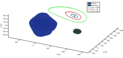
focus, in particular, on the maintenance of a subset of periodic solutions that can be of particular interest for the exploration of a binary system or to conduct deflection and prospection ex-periments (see Fig. 1). Periodic solutions around the dynamic equivalent of the Lagrange points L4 and L5 of the binary sys-tem were shown to be of particular interest to extract surface and subsurface material with laser ablation3) _{. The dynamical}

model in the proximity of the binary system includes the gravity of the two asteroids, the gravity of the Sun and solar radiation pressure. Each spacecraft is equipped with a minimum set of sensors under the assumption of low power and low computa-tional capabilities. Following previous work from the authors each spacecraft is assumed to carry a laser range finder, a cam-era and an inter satellite link that allows sharing information with other spacecraft in the formation and provides range and range rate information.

Two scenarios will be considered in this study: one in which one single spacecraft combines telemetry from Earth with lo-cal measurements, the other in which a formation of spacecraft

autonomously navigate with no measurement from Earth. It will be shown that the combination of camera and laser range finder substantially improves the navigation accuracy and that the intersatellite link allows the formation to autonomously nav-igate and control their position near L4. Given the nonlinear na-ture of the dynamics the paper will propose the use of a gener-alised polynomial algebra4)_{to propagate the uncertainty region.}

The algebra replaces the Unscented Transformation in the Un-scented H-infinity Filter.

1400 1200 1000 800 600

y [m]

400 200 0 -200 -400 1500 1000

x [m]

500 0 -500 100

0 -100 -200 -300 300 200

z [m]

Primary Didymoon A/m = 0.005 A/m = 0.01 A/m = 0.02

Fig. 1. Periodic orbits at L4 in the asteroid binary system.

The paper starts with the description of the dynamics and the measurement model, it will then present the state estimation and data fusion strategy, including the use of the new algebra. Some results and conclusions will complete the paper.

2. Dynamic Model

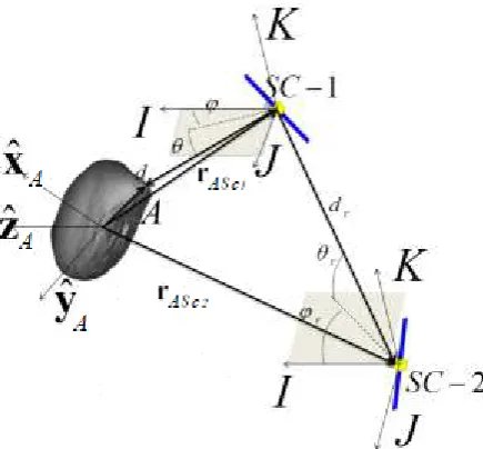
Fig. 2. Reference frame for dynamics and measurement model.

be a homogeneous sphere, the secondary is a homogeneous el-lipsoid with semi-axesaB,bBandcB, rotating around the z-axis with angular velocityωB5).

The gravity field of the secondary asteroid can be expressed as the sum of a spherical field plus a degree and second-order field:6)

U20,22=

µB

δr3

BS ci

"

C20 1− 3 2cos

2_(θ B)

!

+3C22cos2(θB) cos(2ϕB)

i

(1)

whereδrBS ciis the relative position vector between the asteroid B and the spacecraftiin the body-fixed frame B,µBis the as-teroid gravitational constant, the harmonic coefficientsC20and C22are a function of the semi-axes:

C20=− 1 10

2cB2−aB2−bB2

C22= 1 20

aB2−bB2

(2)

andθBandϕBare the longitude and latitude angles respectively:

θB=tan−1

      

zB

p

xB2+yB2

     

; ϕB=tan

−1 yB

xB

!

(3)

The conversion from the body-fixed frame to the reference one is obtained by the simple rotation matrix:

I_R B =

       

cos(ωBt) −sin(ωBt) 0 sin(ωBt) cos(ωBt) 0

0 0 1

       

(4)

wheretindicates the time. The spacecraft is assumed to be sub-ject to the gravitational force of the Sun, solar radiation pressure and the irregular gravity of the binary system. BeingrAthe po-sition of asteroid A,rBthe one of asteroid B,rS the one of the Sun andrS cithe one of the i-th spacecraft all in the chosen ref-erence frame, definingrAS ci =rS ci−rA,rBS ci =rS ci−rBand

rS S ci = rS ci−rS as the relative position vectors from the i-th

spacecraft to the asteroids A and B and the Sun respectively, the nonlinear equations of motion are:

¨

rS Ci= −

µA

krAS c_ik3rAS ci

−

" µ

B

krBS c_ik3 +

I_R B

∂U20,22

∂δrBS ci

!

B

#

rBS ci

− µS krS S cik

3rS S ci+

µS

krSk3

rS +aS RP+u (5)

withµS,µAandµBbeing gravity constants of the Sun, asteroid A and B respectively. The quantityaS RP represents the solar radiation pressure, defined as:

aS RP=CRiSS RP

r1AU

rS S ci

!2

Ai

mS ci ˆ

rS S ci (6)

whererS S ci is the distance of the i-th spacecraft from the Sun,

Ai andmS ci are the spacecraft cross sectional area and mass respectively,CRi is the reflectivity coefficient,SS RPis the solar radiation pressure at 1 AU andr1AUis one astronomical unit in km. The vector u = hux,uy,uz

iT

in equation (5) is a control input, which will be defined later in Section4..

If one considers a formation of 4 spacecraft, the vector equa-tion (5) can be applied to each spacecraft independently and can be re-written in compact form as a system of first order diff er-ential equations:

˙

X= f(X,u) (7)

whereX =

rS c1,˙rS c1,rS c2,r˙S c2,rS c3,r˙S c3,rS c4,r˙S c4T is the state vector containing the position and velocity of all the space-craft.

3. Measurement Model

With reference to Figure 2, it is assumed that each spacecraft is provided with the following set of sensors and measurements: • A camera which provides elevation and azimuth angles of

centroid of the asteroid;

• A laser range finder which measures the distance from the spacecraft to a point on the asteroids surface;

• Inter-spacecraft measurements, which include the relative distance vector between two spacecraft, in terms of range, azimuth and elevation.

In the case of single spacecraft orbiting the system, the inter-spacecraft measurements are substituted by relative range, az-imuth and elevation measurements obtained from a ground sta-tion. Note that in this paper we do not consider standard deep space navigation and tracking methods using, for exam-ple, DOR or∆-DOR. These more realistic measurements will be introduced in future work.

3.1. Camera Model

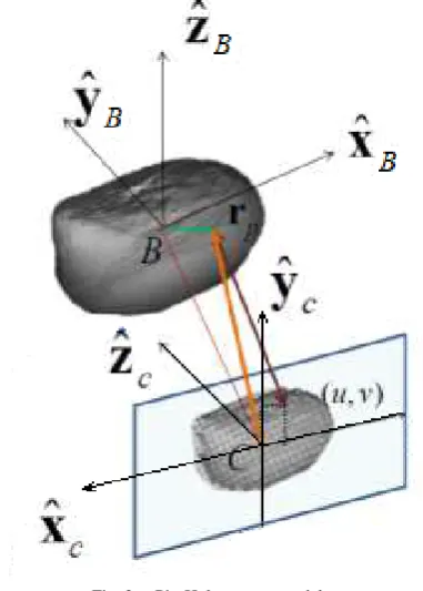
In order to develop the measurement model of the camera, two intermediate reference frames are required as shown in Fig-ure 3:

the three symmetrical body axes defined as three coordi-nate axes7)_.

• Camera coordinate system C{xˆCyˆCzˆC}: the centre C is the perspective projection of the camera, with thezC-axis parallel to the optical axis of the camera and directed to the centre of the asteroid. The image plane is defined as

OC-xCyC.

In this paper, it is assumed that the body reference frame of each spacecraft is aligned with the camera and the attitude is known with a level of precision corresponding to the one of the star tracker.

Fig. 3. Pin-Hole camera model.

A picture is generated by a graphics library according to the state of the system. Then, an ellipse fitting algorithm is used to compute the coordinates of the centroid of the asteroid in camera coordinates. Once the position of the centroid is known, the pointing angles can be computed by:

ϕC =tan−1

xC

f

!

; ψC=tan−1

yC

f/cos (ϕC)

!

(8)

wheref is the focal length of the camera. To these angles those required to go from the camera frame to the spacecraft frame are added. The model for the observation equations used in the filter, neglecting the contribution given by the attitude system, is:

zcamera=

"_ϕ

ψ #

+

"_ζ

ϕ

ζψ

#

(9)

whereζφ,ψ comprise all the errors from attitude and centroid-ing process. Note that here the illumination conditions are not considered, so it is assumed that each spacecraft sees the whole visible surface from its position. This is is reasonable if one as-sumes that a complementary map could be built while starting the orbit acquisition, combining pictures from the whole forma-tion.

3.2. Laser ranging Model

In general, the laser provides range from the spacecraft to a point on the surface of target object and works at a range from 50 m to 50 km.8) _{It is assumed that the laser illuminates the}

point on the surface that corresponds to the centroid derived from the elaboration of the images acquired by the camera.9) This distance is simply given by:

l=krsc−rsur fk (10)

wherersur f is the position of a point on the asteroids surface along the centroid direction. The observation equation of the laser including the measurement noise is:

yl=hl(rsc)+ζl=l+ζl (11)

withζlthe measurement noise. The accuracy of this measure-ment depends on the characteristic error of the sensor, along with a bias defined by the mounting error of the instrument. If the range l is pre-processed in combination with the angular measurements from equation (8), a relative position vector from the spacecraft to the point on the surface can be constructed as

z=

       

l

ϕ ψ       

=

h(rsc)+ζ (12)

wherezis the measurement vector obtained from the combi-nation of camera and laser,h(rsc) is the vector containing the measurement model andζis the total measurement noise vec-tor.

3.3. Inter-spacecraft Measurements

The set of inter-spacecraft measurements is represented by the relative position vector between two spacecraft in the for-mation. Similarly to the model in Section3.2., this is composed of the relative distance, local azimuth and elevation.10) _The

ob-servation equation is given by:

zr=hr

rS c_i, rS c_j=_d

rϕrψrT +ζr (13)

whereζr=

h

ζdrζϕrζψr

iT

is the measurement noise. 3.4. Ground Station Measurements

The set of measurements defined by rangeρ, azimuthϕand elevationψwith respect to the ground station is used to estimate a spacecraft trajectory from Earth. These values are described in the East-North-Zenith reference frame:

ρGS =kρENZk

ϕGS =tan−1

x_ENZ

y_ENZ

!

ψGS =sin−1

z_ENZ

ρ !

(14)

where ρENZ =

x_ENZy_ENZ z_ENZT

is the position vector of the spacecraft measured from ground station. The value of the az-imuth is computed Eastwards from the North direction. The observation equation is given as:

zGS =hGS rS ci, rGS

+ζ

GS =ρGS ϕGS ψGS T_+ζ

4. Control strategy

The control strategy aims at keeping each spacecraft orbiting on a trajectory proximal to the nominal one. Note that this is not an optimal control strategy but it is sufficient to demonstrate the effect of the navigation and data fusion algorithms. The control law is given by the simple PD controller:

u=KP

                 x y z         G −         x y z         N         

+KD

                 ˙ x ˙ y ˙ z         G −         ˙ x ˙ y ˙ z         N          (16)

where the subscripts G and N stand for guidance and naviga-tion respectively, KP is the proportional coefficient and KD is the derivative one. If the actual trajectory of the spacecraft is known, the continuous control in Eq. (16) can be introduced into the full dynamic model in Eq. (5). Here however, the tra-jectory is estimated by the navigation system with the actual position of the spacecraft never known exactly. The predicted estimation is used by the controller to maintain the relative for-mation (shown later in Section 5). Once the controller is in-serted in the spacecraft dynamic model, one obtains a closed loop problem in which the control is performed together with the estimation, and the filter equations incorporate the action of the controller. During the controlled phases, it is assumed that the asteroid trajectory is precisely known; the state variables to be estimated are only those related to the spacecraft in the formation.

5. State Estimation and Data Fusion Strategy

The state estimation process is based on the same Uscented

H∞Filter proposed in.1)

The UHF works on the premise that one can find a good ap-proximation for the a posterioricovariance by propagating a limited set of optimally chosen samples.11) _{Using the}

estima-tion theory formalism, the nonlinear process in Eq. (7) and measurement equations in Section3.can be discretised in time and written as:

xk+1= f(xk, uk)

yk=h(xk, vk) (17)

wherevk is the measurement noise. The initial conditions are the estimated position and velocity from the filter at timetk. The UHF relies on the unscented transformation to propagate a set of suitable sigma points, drawn from thea prioricovariance matrix. The set of sigma pointsχare given as:

χi=

                         ˜

xk i=0

˜ xk+

q

n+kU HF

_P

k+Qk

i

i=1, 2, ..., n

˜ xk−

q

n+k_{U HFP}

k+Qk

i

i=n+1, ..., 2n

(18) whereχis a matrix consisting of (2n+1) vectors withk_{U HF} =

α2

U HF n+λU HF

−n, wherek_{U HF}is a scaling parameter, and con-stantαU HF determines the extension of these vectors around ˜xk. We setαU HF equal to 10−2andλU HF is set equal to (3n). The

sigma points are transformed or propagated through the nonlin-ear function, the so-called unscented transformation, to give:

χi,k+1= f χi,k, uk

Yi=h χi,k, vk i=0, 1, , ..., 2n (19)

The mean value and covariance of y are approximated using the weighted mean and covariance of the transformed vectors11)

ˆ y=

2n

X

i=0

W_i(m)Yi

Py= 2n

X

i=0

W_i(c)(Yi−yˆ) (Yi−yˆ)T

(20)

whereW_i(m) andW_i(c)are the weighted sample mean and co-variance given by:

W₀(m) =k_{U HF}/(n+k_{U HF})

W₀(c) =k_{U HF}/(n+k_{U HF})+(1−α2

U HF+βU HF)

W_i(m) =W_i(c)=kU HF/[2(n+kU HF)], i=1, 2, ..., 2n

(21)

andβU HFis used to incorporate prior knowledge of the distri-bution withβU HF =2.

12)_{The predicted mean of the state vector}

˜

x−_k, the covariance matrix ˜P−_k, and the mean observation ˜y−_k can be approximated using the weighted mean and covariance of the transformed vectors:

χi

k|k−1 =f

χi

k−1, uk

˜ x−_k =

2n

X

i=0

W_i(m)χi_k|k−1

P−_k = 2n

X

i₌0

W_i(c)hχi_k|k−1−x˜−_ki hχ_ki_|k−1−x˜−_kiT+Qk

Yi_k|k−1=hχi_k|k−1

˜ y−_k =

2n

X

i=0

W_i(m)Yi_k|k−1

(22)

The updated covariancePy,kand the cross correlation matrix Pxy,kare:

Py,k= 2n

X

i=0

W_i(c)hYi_k|k−1−y˜−_ki hY_ki_|k−1−y˜−_kiT+Rk

P−_k = 2n

X

i=0

W_i(c)hχi_k|k−1−x˜−_ki hYi_k|k−1−y˜−_kiT

(23)

Finally, the filter state vector ˜xk and covariance updated ma-trixPx,kare represented as follows:

˜

xk=x˜−k +K(yk−y˜k)

P+_k−1 =P−_k−1+P−_k−1Pxy,kR−_k1

P−_k−1Pxy,k

T

−ϑkId

K=Pxy,kP−_y,k1

whereKis the Kalman gain matrix, ϑk is the performance bound of theH∞filter, andRkis a suitable matrix which, in the case of a normal distribution, coincides with the measurement noise covariance matrix at time step k. In order to assure that the covariance matrix is positive definite this value is calculated at each iteration as:

ϑ−1

k =ξmax

     

eig

P−_k−1+P−_k−1Pxy,kR−_k1

P−_k−1Pxy,k

T!−1_

    

(25) As one can see from the set of equations (24), the perfor-mance bound has no direct effect on the calculation of the gain and on the update step for the estimated state. Nonethelessϑk modifies the shape of covariance matrix update, which, in turn, generates a different distribution of the sigma points. In this way, the propagation and the update step at the following time step will be directly influenced by the value of the performance bound.

5.1. Filtering with Chebyshev Polynomial Algebra The use of an unscented transformation to calculate the prop-agated covariance matrix was shown to be a good solution to re-cover some nonlinearities in the dynamics. On the other hand, the Unscented Transformation starts from the strong assump-tion of symmetric Gaussian distribuassump-tion and provides anyway a second order approximation to the distribution of the propa-gated states.

In order to better capture the nonlinearities in the dynamics, in this paper, we propose the use of a recently developed poly-nomial algebra based on Chebyshev polypoly-nomial expansions.

The function spacePn,d(α)=< αI(b)>whereb∈Ω⊂Rd,

I = (i1, . . . ,id) ∈ Nd+ and|I| = Pdj=1ij ≤ n, is the space of

polynomials in theαbasis up to degreenindvariables. This space can be equipped with a set of elementary arithmetic oper-ations, generating an algebra on the space of polynomials such that, given two elementsA(b),B(b) ∈ Pn,d(α) approximating any two real multivariate functions fA(b) and fB(b), it stands that

fA(b)⊕fB(b)∼A(b)⊗B(b), (26) where⊕ ∈ {+,−,·, /}and⊗is the corresponding operation in Pn,d(αi). This allows one to define the algebra (Pn,d(αi),⊗), of dimension dim(Pn,d(αi),⊗)=Nd,n =

_n+d

d

, the elements of which belong to the polynomial ring indindeterminatesR[b] and have degree up ton. Each elementP(b) of the algebra, is uniquely identified by the set of its coefficientsp ∈RNd,n _such that

P(b)= X I,|I|≤n

pIαI(b). (27)

In the same way as for arithmetic operations, it is possi-ble to define a composition rule in the polynomial algebra and hence the counterpart, in the algebra, of the elementary func-tions{sin(y),cos(y),exp(y),log(y), ...}. Differentiation and inte-gration operators can also be defined. By defining the initial conditions and model parameters of the dynamics as element of

the algebra and by applying any integration scheme with opera-tions defined in the algebra, at each integration step is available the polynomial representation of the state flow. The main ad-vantage of the method is in the control of the trade-offbetween computational complexity and representation accuracy at each step of integration. Furthermore, sampling and propagation are decoupled, therefore, irregular regions can be propagated with a single integration, provided that a polynomial expression is available. It has been shown that the polynomial algebra ap-proach presents overall good performance and scalability (with respect to the size of the algebra) compared to its non-intrusive counterpart. On the other hand, being an intrusive method, it cannot treat the dynamics as black box. Its implementation re-quires operator overloading for all the algebraic operations and elementary functions defining the dynamics, making it more difficult to implement than a non-intrusive method.

The algebra is used to propagate the set of variated states in place of the Unscented Transformation. The idea is to replace the numerically integrated states:

Xk+1,i=f(Xk,i,uk,i), (28)

wherefis the integration of the dynamics from statekto state

k+1 at samplei, with the full polynomial representation of the set of final states:

Xk+1,i=P(Xk,i,uk,i), (29) where the polynomialsPare defined as in Eq.(27). The rest of the filter remains unchanged.

5.2. Multi-spacecraft Data Fusion Process

Having defined the filtering and control processes, each spacecraft needs to data fuse its own measurements and the in-formation shared with the other spacecraft. This section de-scribes the data fusion process implemented to address this is-sue. Each spacecraft receives the whole set of measurements coming from all the members and builds the necessary ma-trices for the filtering process. The analysis in this paper is limited to the case in which inter-spacecraft measurements are synchronous with a single common time tag. In the case of asynchronous measurements a different time tag is associated to each measurement.

The information sharing and fusion is achieved by exploit-ing the inter-spacecraft measurement of equation (13). In fact, when a new inter-spacecraft measurement is available for spacecrafti, spacecraftjtransmits back the current estimation of its own state to be used in the estimation process. This is nec-essary because the position of spacecraftjis required in order to compute the predicted relative distance measurements.

The estimation process, for each spacecraft, can be described through the following 3 main steps:

1. At initial timet0, each spacecraft initialises its filter with

the initial guesses on the state,X0, and covariance,P0The sigma points, relative to all the sensors mounted on the spacecraft, are generated according to the UHF implemen-tation algorithm;

2. The estimated state and the sigma points are propagated fromtktotk+1;

3. At timetk+1, predicted and actual measurements are

knowledge. If the number of measurements is lower than the predicted number, only the consistent measurements between the two steps are considered in the update step. This is obtained by removing the predicted measurements and the correspondent columns and rows in the filter gain.

6. Results

The binary asteroid system chosen as environment for the simulations is 65803 Didymos, whose parameters are listed in Table 1. For simplicity reasons, the orbital motion of the sys-tem around the Sun has been considered circular and laying in the ecliptic. The dimensions and gravitational parameters are chosen according to the current knowledge of the system. The secondary body is tidal locked. The cameras are assumed to

Semi-major axis a 1.6446 AU

Eccentricity e 0.3838

Inclination i 3.4077 deg

RAAN Ω 73.2219 deg

Argument of periapsis ω 319.2516 deg

Orbital period TD 2.11 yr

Distance AB dAB 1.18 km

System rot. period TAB 11.92 h

Grav. param. A µA 3.4908∗10−8km3/s2 Physical dimensions aA,bA,cA 387.5, 387.5, 387.5 m

Rotational velocity ωA 2.26 h

Grav. param. B µB 3.1781∗10−10km3/s2 Physical dimensions aB,bB,cB 81.5, 62.7, 52.2 m

Rotational velocity ωB 11.92 h

Table 1. Orbital and physical parameters for 65803 Didymos

have a resolution of 300x300 pixels, with a field of view of 50 degrees. Table 2 summarizes the measurement errors used in the simulations. The LIDAR range error is set to 10 m accord-ing to Kubota et al. (2003), and a precision of 2 m is used for the inter-spacecraft LIDAR range measurement error. Angular measurements and attitude errors are from Yim et al. (2000). It is assumed that the measurements from Earth are taken from an ideal ground station positioned at (0.0 deg latitude and 0.0 deg longitude) with minimum served elevation of 0.0 deg. The mass of each spacecraft is constant and equal to 500 kg, the maximum cross section area is 20m2_{and reflectivity coefficientC}

Ris as-sumed equal to 2. The initial estimated state is always equal to the real initial state augmented by some bias. Specifically, the position components are always increased by 100m and the ve-locity ones by 1m/s. The initial covariance matrix is a diagonal matrix whose elements are equal to the square of twice the ini-tial error for each component of the state. As a final remark, for all the test cases the application of the control is delayed by 2 hours, in order to allow the filters to converge. In both the sce-narios presented the spacecraft will be required to keep a stable trajectory close to the Lagrangian point L4 of the binary system. This point, due to the irregularities in the gravitational field of the system and the presence of the Sun (gravitational pertur-bation and radiation pressure) is unstable and the spacecraft is soon swept away if no control is applied.

Sensors errors 1−σ

Camera pixelisation ζϕ,ψ 10−3_rad

LIDAR ζl 10m

Inter-sat distance ζdrel 2m Inter-sat angles ζϕrel,ψrel 10

−3_rad

GS range ζρGS 20m

GS angles ζϕGS,ψGS 5.5 10

−3_deg

Table 2. Sensors errors

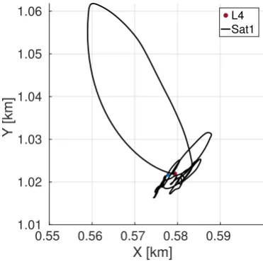
6.1. Case 1: single spacecraft with ground station link In this scenario, the satellite is positioned at the Lagrangian point L4 and the initial conditions are such that the ground sta-tion sees the spacecraft at the zenith. Figure 4 shows the tra-jectory of the spacecraft around the Lagrangian point in the ref-erence frame rotating with the binary system. In the first two hours, before the control law takes over, the spacecraft starts drifting away from the Lagrangian point in direction top-left. When the spacecraft reaches the furthermost point from the initial position, the control starts acting and the spacecraft is pushed in proximity of L4. A blue marker indicates the final position of the spacecraft at the end of the simulation. The os-cillatory noisy motion of the spacecraft around the Lagrangian point is due to the nature of the control law and the uncertainty in the estimation of its state. Figure 5 reports the error in the estimation of the position of the spacecraft. It can be seen that, after a short transient, the estimation converges to a value of 6.96 m. Such a value for the position error is of the same order

0.55 0.56 0.57 0.58 0.59

X [km] 1.01

1.02 1.03 1.04 1.05 1.06

Y [km]

L4 Sat1

Fig. 4. Case 1: trajectory of the spacecraft around L4

0 2 4 6 8 10 12

Time [h]

100

101

102

103

Error [m]

Sat-1

Error RMS Covariance 1- σ

of magnitude expected from the uncertainty on the measure-ments of the Camera/LIDAR combination. It can be seen, then, that the use of such a sensor, together with appropriate tuning of the weighting coefficients in the information from the mea-surements, is capable of compensating the much higher error induced by the measurements from the ground station. 6.2. Case 2: formation of 4 spacecraft

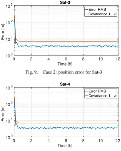
In this scenario, a formation of 4 spacecraft is positioned around the Lagrangian point L4. The initial conditions are such that all the spacecraft has the sameycoordinate of L4 but a bias one the x component. These biases are+10m for Sat-1,+20m for Sat-2, -10m for Sat-3 and -20m for Sat-4. Figure 6 shows the evolution of the trajectories, while Figures 7 to 10 show the error in the estimation of the position for all the 4 spacecraft. The results obtained are very similar to the ones shown in

0.54 0.56 0.58 0.6 0.62

X [km]

1 1.01 1.02 1.03 1.04 1.05 1.06 1.07

Y [km]

L4 Sat1 Sat2 Sat3 Sat4

Fig. 6. Case 2: trajectories of the 4 spacecraft in proximity of L4

0 2 4 6 8 10 12

Time [h]

100

101

102

103

Error [m]

Sat-1

Error RMS Covariance 1- σ

Fig. 7. Case 2: position error for Sat-1

0 2 4 6 8 10 12

Time [h]

100

101

102

103

Error [m]

Sat-2

Error RMS Covariance 1- σ

Fig. 8. Case 2: position error for Sat-2

the previous case. This is a proof that the set of measurements used, LIDAR, camera and inter-satellite link, is capable of mak-ing the formation navigate autonomously without the need of any Earth-based information. The evolution of the trajectories

0 2 4 6 8 10 12

Time [h]

100

101

102

103

Error [m]

Sat-3

Error RMS Covariance 1- σ

Fig. 9. Case 2: position error for Sat-3

0 2 4 6 8 10 12

Time [h]

100

101

102

103

Error [m]

Sat-4

Error RMS Covariance 1- σ

Fig. 10. Case 2: position error for Sat-4

in Figure 6 shows that all the spacecraft have a wider oscillation in one direction (bottom left to top right). Such direction is the one that leads to the primary asteroid, the one used for the mea-surements. This agrees with the values of the error components of the LIDAR/camera measurements, since the uncertainty on the distance is greater that the transverse one due to the uncer-tainty on the pointing angles. The average computational time for these simulations was of 85.8168 seconds.

6.3. Case 3: formation of 4 spacecraft with Chebyshev al-gebra propagation

In this test case, the use of the Chebyshev algebra, described in Section5.1., is employed in the estimation process. The poly-nomial representation is carried on by the use of third order polynomials in the 6 variables of the dynamical state. Before each propagation, from time tk to timetk+1, upper and lower

0 2 4 6 8 10 12 Time [h]

100

101

102

103

Error [m]

Sat-4

Error RMS Covariance 1- σ

Fig. 15. Case 3: position error for Sat-4

0.54 0.55 0.56 0.57 0.58 0.59 0.6 0.61

X [km] 1

1.01 1.02 1.03 1.04 1.05 1.06

Y [km]

L4 Sat1 Sat2 Sat3 Sat4

Fig. 11. Case 3: trajectories of the 4 spacecraft in proximity of L4

0 2 4 6 8 10 12

Time [h]

100

101

102

103

Error [m]

Sat-1

Error RMS Covariance 1- σ

Fig. 12. Case 3: position error for Sat-1

0 2 4 6 8 10 12

Time [h]

100

101

102

103

Error [m]

Sat-2

Error RMS Covariance 1- σ

Fig. 13. Case 3: position error for Sat-2

0 2 4 6 8 10 12

Time [h]

100

101

102

103

Error [m]

Sat-3

Error RMS Covariance 1- σ

Fig. 14. Case 3: position error for Sat-3

7. Conclusion

The paper presented some first results on the autonomous navigation of a formation of spacecraft in the proximity of a binary system. The formation was specifically trying to main-tain the position of the spacecraft around L4. It was demon-strated that with a combination of optical measurements and inter-spacecraft links the formation could be controlled within an error of few meters. The next step will be to test delays and failures in the sensors and the communication chain as previous done for the case of a single asteroid. The paper introduced also the use of a generalised polynomial algebra based on Cheby-shev polynomials for the propagation of the dynamics. In fu-ture work the potentiality of the algebra will be extended to the propagation of the full probability distribution rather than lim-iting the construction of the filter only on the first two statistical moments.

References

1) Vetrisano M., Vasile M. Autonomous Navigation of a Spacecraft For-mation in the Proximity of an Asteroid. Advances in Space Research, Volume 57, Issue 8, 15 April 2016, Pages 17831804

2) Vetrisano M., Vasile M., Colombo C., Asteroid Rotation and Orbit Control via Laser Ablation. Advances in Space Research, Volume 57, Issue 8, 15 April 2016, Pages 17621782.

3) Thiry, N. and Vasile, M., Binary Asteroid Manipulation with Laser Ablation. HPLA/DE, Santa Fe, 4-6 April 2016.

4) Riccardi, A., Tardioli, C., Vasile, M., An Intrusive Approach to Un-certainty Propagation in Orbital Mechanics Based on Tchebycheff Polynomial Algebra. Astrodynamics Specialists Conference, AAS 15-544, Veil, Colorado, USA, 9-13 August 2015

5) Scheeres, D.J. Orbit Mechanics about Asteroids and Comets. Journal of Guidance, Control and Dynamics, 2012, 35(3): 987-997. 6) Hu, W. and Scheeres, D.J. Spacecraft motion about slowly rotating

as-teroids. Journal of Guidance, Control and Dynamics 25 (4), JulyAu-gust 2002, 765775.

7) Li, S., Cui, P.Y., Cui, H.T. Vision-aided inertial navigation for pin-point planetary landing. Aerospace Science and Technology, 2007, 11(6):499-506.

8) Kubotaa, T., Hashimotoa, T., Sawai, S., Kawaguchib, J., Ninomiyaa, K., Uoc, M., Babac, K. An autonomous navigation and guidance sys-tem for MUSES-C asteroid landing. Acta Astronautica 52 (2003) 125 131.

9) Dionne, K. Improving Autonomous Optical Navigation for Small Body Exploration Using Range Measurements. AIAA 2009-6106. AIAA Guidance, Navigation, and Control Conference, 10 - 13 Au-gust 2009, Chicago, Illinois.

10) Alonso, R., Du, J., and Hughes, Y Relative Navigation for Formation Flying of Spacecraft. Proceedings of the Flight Mechanics Sympo-sium, NASA-Goddard Space Flight Center, Greenbelt, MD, 2001, pp. 115-129.

11) Julier, J. K. Uhlmann and Durrant-Whyte, H.F. A new approach for filtering nonlinear systems, Proceedings of the American Control con-ference, Seattle, Washington, 1995.