Laboratory infrastructure driven key performance indicator development using the Smart Grid Architecture Model

(1)

LABORATORY INFRASTRUCTURE DRIVEN KEY PERFORMANCE INDICATOR

DEVELOPMENT USING THE SMART GRID ARCHITECTURE MODEL

M.H. Syed, E. Guillo, S.M. Blair & G.M. Burt T.I. Strasser, H. Brunner O. Gehrke J. E. Rodriguez-Seco University of Strathclyde – UK AIT – Austria DTU – Denmark Tecnalia – Spain

[email protected], [email protected], [email protected], [email protected]

ABSTRACT

This paper presents a methodology for collaboratively designing laboratory experiments and developing key performance indicators for the testing and validation of novel power system control architectures in multiple laboratory environments. The contribution makes use of the smart grid architecture model (SGAM) as it facilitates the integration of individually developed control functions into a consolidated solution for laboratory validation and testing. The experimental results obtained across multiple laboratories can be efficiently compared, when the proposed methodology is adopted and thus the paper offers means of support for improved cooperation in smart grid validation and round robin testing.

INTRODUCTION

Within Europe, multiple research organizations are collaborating to address challenges posed by large scale integration of renewable energy resources and to support the broader European Union Energy Policy of decarbonizing the power grid. It is vital that the potential solutions for controlling the future grid are systematically validated in realistic laboratory conditions to accelerate their confidentadoption.

The integration of multiple software and hardware controllers into a consolidated solution for laboratory validation and testing is complex due to the requirements of developing consistent functional interfaces between controllers and ensuring real-time operation [1]. Therefore, a structured process must be followed when assessing the performance of novel solutions, which requires:

 defining key performance indicators (KPIs)

 measuring the defined KPIs in laboratories

 comparing the measured KPIs with a business as usual (BAU) case.

Testing activities are sometimes performed across multiple laboratories [2], which brings various benefits such as exposure to a wider variety of hardware testing environments, communication protocols and testing procedures that collectively have the potential to increase the robustness of the tested system. Therefore, it is of critical importance to formulate KPIs that do not depend on the peculiarities of individual laboratory setups and capabilities, in order to ensure that the results are comparable. This is a challenging task; for example, many relevant indicators of power system control

performance, such as the rate of change of frequency during disturbances, are linked to time constants which are highly specific to the system inertia, unit capabilities and signal delays inherent to the physical power system being measured [3-5].

Typically, for laboratory validation and testing of power system controllers, multiple functions need to be integrated within the laboratory environment. These intelligent solutions comprise more than one inter-dependent function encompassing multiple domains that are developed independently by domain experts and brought together for integration within the laboratory for validation and testing. By using the smart grid architecture model (SGAM) [6] the interdependencies of the different functions are more clearly exposed and therefore the development of the KPIs required for testing across multiple facilities can be performed in a meticulous manner. A methodology for developing suitable KPIs using the SGAM is presented in this paper. This paper builds upon the work presented in [7], and advances the state-of-the-art by demonstrating a structured approach for multi-laboratory collaborative KPI development.

METHODOLOGY FOR KPI DEVELOPMENT

A three-stage methodology that uses SGAM as a tool has been developed to formally determine an experimental plan and KPIs, as illustrated in Figure 1. The methodology follows a structured approach wherein the KPIs for a smart grid control solution evaluation by the laboratory infrastructure are developed further. The three stages of the methodology are described in detail in the following subsections, and are further illustrated by the Case Study.

Smart Grid Control Solution Description

SGAM Function and Information Layers per Solution

Reference Power System

Laboratory Infrastructure

SGAM Component, Communication and Information Layers per Lab

Test Cases and KPI Extraction

S

ta

g

e

I

S

ta

g

e

I

S

ta

g

e

I

II

(2)

Stage I

In the first stage of the methodology, the functions involved in the smart grid control solution are identified and mapped onto the corresponding zones and domains of the functional layer of the SGAM. A description of how a distributed control solution can be mapped on to the functional layer of SGAM has been detailed in [7]. The information that is exchanged between the different functions is identified and the “business context view” of the SGAM information layer is developed.

In the case where multiple partners will be validating the proposed control solution in their respective laboratories, this stage is undertaken by each of the partners independently. Once these two layers of SGAM have been developed by each of the partners, the layers can be shared between the partners and an exercise to consolidate the control solution is undertaken. This process ensures that the control solution is understood consistently across all the partners and avoids any confusion at a later stage.

Stage II

In order to test and validate the smart grid control solution in the laboratory, a reference power network is required. In most of laboratories, the reference power network is the power network available within the laboratory. However, in laboratories capable of conducting power hardware-in-the-loop simulations (PHIL), a larger power network can be simulated, with the laboratory network being a small part of the larger virtually simulated network. In such cases, a reference power system is chosen based on the individual laboratory capabilities.

Once the reference power network has been selected, the next step is to establish the periodic refresh rate for the information that is exchanged between the functions. This rate depends upon the application of the control solution and is usually determined by the control solution developers. Depending upon the data refresh requirements, the components – i.e. the intelligent electronic devices (IEDs) – in the laboratory that can be utilized for the implementation of the functions are identified. Once the components have been identified, the communication protocols and data formats supported by the components are summarized. This enables the population of component layer, communication layer and canonical view of information layer of SGAM. Having all the layers of SGAM populated provides a full view of the testing environment with the implemented control functions that will facilitate the definition of experiments.

Stage III

In the third stage of the methodology, a reference event to be simulated for evaluating the performance of the developed control solution is chosen. Furthermore, to be able to appraise the performance of the novel developed controller, it is important to compare the results obtained

with a BAU case. Once the reference event and the BAU case have been selected, a short narrative on the experiment that will be conducted to test the smart grid control solution in the laboratory is drafted. This allows for the detailed test cases to be described and for the KPIs to be refined.

CASE STUDY

To address the need of a new power system architecture that is capable of supporting a decarbonized grid, the ELECTRA IRP project has introduced the Web of Cells (WoC) architecture [8]. The aim of the WoC architecture is to support secure system-wide operation by means of distributed control among distinct regions of the power network, called cells, thereby improving the observability, controllability and reliability of future power systems. WoC requires the division of a power system into smaller control entities (compared to the present day load frequency control (LFC) areas) responsible for optimized operation of locally available flexibility to manage voltage and balance deviations. Each cell should address deviations originating within itself i.e. solving local problems locally. For this purpose, novel frequency and voltage control solutions for the WoC architecture have been developed.

The proposed methodology has been applied to obtain the KPIs for experimental evaluation of the developed novel frequency and voltage control solutions. In this case study, one of the frequency control solutions, called the balance restoration control (BRC), will be utilized to present an example use of the proposed methodology. More details on the control solution can be found in [7]. ELECTRA IRP involves a total of eleven partners with state-of-the-art laboratory facilities. This methodology has been followed by each of the laboratory partners, however due to restriction in space, only the example generated by University of Strathclyde using the Distribution Network and Protection (D-NAP) Laboratory is presented. The outcomes of the different stages are described below.

Stage I

As per the methodology, the functions and the information that are exchanged between the functions in BRC are identified and the functional and business context view of the information layer are populated (as shown in Figure 2). As the frequency control solution developed within ELECTRA IRP aims to utilize the flexibility available within distribution networks, the generation and transmission domains of SGAM have been omitted. Similarly, the control solution developed does not involve any wholesale market operation and therefore the market zone has been omitted at this stage.

Stage II

(3)

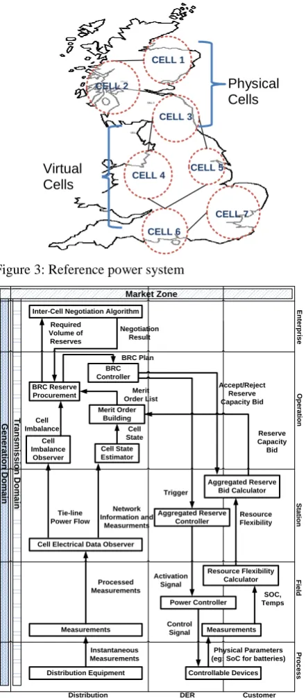
Figure 3: Reference power system

Cell Imbalance

Observer

Tie-line Power Flow Cell Imbalance

Resource Flexibility

Physical Parameters (eg: SoC for batteries) Controllable Devices

Measurements Power Controller

SOC, Temps Aggregated Reserve

Bid Calculator BRC Reserve

Procurement

Reserve Capacity Bid Accept/Reject

Reserve Capacity Bid

Cell Electrical Data Observer Cell State Estimator

Distribution Equipment Measurements

Network Information and

Measurments Cell State

Processed Measurements

Instantaneous Measurements

G

e

n

e

ra

tio

n

D

o

m

a

in

T

ra

n

s

m

is

s

io

n

D

o

m

a

in

Distribution DER Customer

P

ro

c

e

s

F

ie

ld

S

ta

tio

n

O

p

e

ra

tio

n

E

n

te

rp

ri

s

e

Negotiation Result Inter-Cell Negotiation Algorithm

Merit Order Building

Resource Flexibility Calculator Merit

Order List

Trigger

Control Signal Required

Volume of Reserves

Aggregated Reserve Controller

Activation Signal BRC

Controller BRC Plan

Market Zone

Figure 2: Business context view of information layer (function layer is without the exchange of information)

within ELECTRA IRP can be found at [9]. With the ability to conduct real-time PHIL simulations in D-NAP, a reduced dynamic model of the UK power system, as shown in Figure 3, has been selected as the reference power system [10]. The UK power system has been split into seven cells to incorporate the WoC architecture. Three of the cells will be emulated by the power equipment in the laboratory and four cells will be simulated in real-time.

For the purpose of illustration, the refresh rates of inputs and outputs for two functions have been presented in Table 1. Based on the refresh rates, two components for implementation of the functions have been identified as shown in Table 1. This enables development of the component layer of SGAM as shown in Figure 4a. The control functions for all seven cells are to be implemented on the same components (i.e. the cell imbalance error function for all cells will be implemented within IED-3 and the aggregated reserve bid calculator function for all cells will be implemented within IED-1). The power equipment is mapped onto the process zone of SGAM. As explained in [7], one component layer for each cell must be developed. Therefore, the various power equipment that will be utilized within the laboratory have been presented as shown in Figure 4b. The supported communication protocols and data formats for selected laboratory components are summarized in Table 2. This allows for the communication and the canonical view of the information layer to be populated as shown in Figure 4c and 4d, respectively. The available environments for the implementation of the control functions are also captured in Table 2. This allows for the function development team (which may be different to the laboratory owner) to decide upon the platform to use for implementing the functions. As can be seen from Table 2, more than one implementation platform, communication protocol and data format might be available for each laboratory component. However, in the SGAM layer, only the implementation environment, communication protocol and data format that is preferred by the laboratory is illustrated.

Stage III

[image:3.595.55.276.103.607.2]

As a frequency control solution is under consideration in this paper, a reference frequency event needs to be simulated for the purpose of evaluating the performance Table 1: Laboratory component identification

Function Inputs (In) Outputs (Out) In Refresh Rate Out Refresh

Rate

Laboratory Component

Cell Imbalance Observer

Tie-line power flow

Cell imbalance Continuous Event based IED-3 (Host PC)

Aggregated Reserve Bid Calculator

Resource flexibility

Reserve capacity bids

Hourly Hourly IED-1 (Host PC)

Table 2: Laboratory component supported communication protocols and data formats

Lab Component Available implementation environment Communication protocols Data format/model

IED-1 (Host PC) IED-1 (Host PC) IED-1 (Host PC)

MATLAB (Simulink/M-File), Python MATLAB (Simulink/M-File), Python

C/C++, Python, Java

UDP TCP IEC 61850 GOOSE

Custom Data Format Custom Data format

IEC 61850-7-4 CELL 1

CELL 2

CELL 3

CELL 4

CELL 2

CELL 5 CELL 3

CELL 4

CELL 6

CELL 7 Physical Cells

[image:3.595.46.551.643.769.2]

(4)

Cell Imbalance Observer Tie-line Power Flow Cell Imbalance Resource Flexibility Physical Parameters (eg: SoC for batteries) Controllable Devices Measurements Power Controller SOC, Temps Aggregated Reserve Bid Calculator BRC Reserve Procurement Reserve Capacity Bid Accept/Reject Reserve Capacity Bid

Cell Electrical Data Observer Cell State Estimator Distribution Equipment Measurements Network Information and Measurments Cell State Processed Measurements Instantaneous Measurements G e n e ra tio n D o m a in T ra n s m is s io n D o m a in

P ro c e s s F ie ld S ta tio n O p e ra tio n E n te rp ris e Negotiation Result Inter-Cell Negotiation Algorithm

Merit Order Building Resource Flexibility Calculator Merit Order List Trigger Control Signal Required Volume of Reserves Aggregated Reserve Controller Activation Signal BRC Controller BRC Plan Market Zone

IED-1 (Host PC) Matlab (Simulink/M-File)

IED-2 (ADI RTS) Matlab (Simulink/M-File)

ADI ADvantage DE/VI IED-3 (Host PC) Matlab (Simulink/M-File) Market Zone Enterprise Zone Operation Zone Field Zone P ro c e s s

Generation Transmission Distribution DER Customer

Controllable Devices Distribution Equipment Load Bank

(40kW) Distribution Cabinet 1

C e ll 1 Physical Cells Triphase 90kVA Market Zone Enterprise Zone Operation Zone Field Zone P ro c e s s

C e ll 2 Triphase 15kVA Market Zone Enterprise Zone Operation Zone Field Zone P ro c e s s

C e ll 3 _SG 2kVA Market Zone Enterprise Zone Operation Zone Field Zone P ro c e s s

Controllable Devices Distribution Equipment Load

Models

Transmission, Distribution Lines & Transformer Models

Gen Models

Virtual Cells : RTDS Cell 4, Cell 5, Cell 6 & Cell 7

(a) Component layer (b) Component layer: process zones of each cell

Cell Imbalance Observer Tie-line Power Flow Cell Imbalance Resource Flexibility Physical Parameters (eg: SoC for batteries) Controllable Devices Measurements Power Controller SOC, Temps Aggregated Reserve Bid Calculator BRC Reserve Procurement Reserve Capacity Bid Accept/Reject Reserve Capacity Bid

ADI ADvantage DE/VI IED-3 (Host PC) Matlab (Simulink/M-File) UDP UDP UDP U D P U D P U D P U D P U D P U D P U D P U D P U D P Cell Imbalance Observer Tie-line Power Flow Cell Imbalance Resource Flexibility Physical Parameters (eg: SoC for batteries) Controllable Devices Measurements Power Controller SOC, Temps Aggregated Reserve Bid Calculator BRC Reserve Procurement Reserve Capacity Bid Accept/Reject Reserve Capacity Bid

ADI ADvantage DE/VI IED-3 (Host PC) Matlab (Simulink/M-File) UDP UDP UDP U D P U D P U D P U D P U D P U D P U D P U D P U D P

Custom Data Format

(5)

of the developed control solution. A number of occurrences of ~1 GW generation loss have been experienced by the Great Britain grid within the last year and therefore a generation loss of 1 GW is selected as the reference event [11]. The frequency control implemented by ENTSO-E [12] within the European grid has been selected as the BAU case.

Smart grid laboratories are not identical in terms of equipment, architecture and capabilities. When multiple laboratories are presented with a control solution, each laboratory has a different perspective in terms of its implementation. The results obtained from the experimental evaluation from different laboratories is valuable, however it is often difficult to compare results obtained independently from two laboratories. The proposed methodology helps multiple laboratories to design experiments together ensuring consolidation and consistency in perspective at every stage, thereby enabling the results to be comparable.

As has been mentioned earlier, the three stages of the methodology have been exercised by all the laboratory partners within the ELECTRA IRP project. One of the KPIs that required a consistent definition was the time for frequency restoration following the reference incident. The reference power system and the reference event are different for each of the laboratory as they are selected based on the capability of the individual laboratory. For the basis of comparison of results between laboratories, an improved KPI/metric can be formulated:

𝑇𝑟𝑎𝑡𝑖𝑜 =

(Time for frequency restoration)𝐵𝑅𝐶

(Time for frequency restoration)𝐵𝐴𝑈 By means of taking a ratio between the two response times, the impact of the differences of the implemented laboratory systems are minimized, making the KPI comparable between the laboratories.

CONCLUSIONS

In this paper, a structured methodology for development of KPIs driven by laboratory infrastructure is proposed. As per this methodology, any intelligent solution to be tested is first represented using the Smart Grid Architecture Model (SGAM) followed by adding the representation of the laboratory infrastructure which will test and validate the solution. The detailed mapping process captures the requirements of the controllers and the capabilities of the laboratory infrastructure. Using these outputs, consistent, appropriate and measurable KPIs can be extracted.

Furthermore, for the first time, an extensive SGAM modelling process has been undertaken on multiple smart grid laboratories. This has demonstrated the value of the proposed methodology for communicating research infrastructure features for integration of test equipment and control solutions. The combined representation of control systems and laboratories using the SGAM enables the transition from the design of radical grid control solutions, to their convincing evaluation and validation.

The ongoing project effort within ELECTRA IRP is directed towards validation of novel WoC controls and utilization of the KPIs, and thus provides increasing evidence to validate the proposed methodology. Experiments will be conducted in at least two smart grid laboratories, and the KPIs will be measured and compared to quantify the impact of the control paradigm.

Acknowledgments

The work in this paper has been supported by the European Commission under the FP7 ELECTRA IRP (grant no: 609687). Any opinions, findings and conclusions or recommendations expressed in this material are those of the authors and do not necessarily reflect those of the European Commission.

REFERENCES

[1] T. Strasser, et al., 2016, “Towards holistic power distribution

system validation and testing- an overview and discussion of different possibilities”, e & i elecktrotechnik und informationstechnik, 1-7.

[2] J. Johnson, et al., 2014, “Collaborative development of

automated advanced interoperability certification test

protocols for PV smart grid integration”, Proceedings of EU

PVSEC, Amsterdam, The Netherlands, 22-26.

[3] A. Kosek et al., 2014, “RTLabOS dissemination activities”,

http://orbit.dtu.dk/files/104280390/D4.2DisseminationActivit ies.pdf accessed 12 January 2017

[4] M. Buscher, et al., 2015, “Using large-scale local and

cross-location experiments for smart grid system validation”,

Proceedings of 41st Annual Conference of the IEEE Industrial Electronics Society IECON, Yokohama, 4621-4626.

[5] M. Stevic, et al., 2015, “Development of a

simulator-to-simulator interface for geographically distributed simulation of power systems in real time”, Proceedings of41st Annual Conference of the IEEE Industrial Electronics Society IECON, Yokohama, 5020-5025.

[6] Smart Grid Coordination Group (SG-CG) Reference

Architecture Smart Grid, CEN, CENELEC, and ETSI, Nov. 2012.

[7] E. Guillo-Sansano, et al., 2016, “Transitioning from

centralized to distributed control: using SGAM to support a collaborative development of web if cells architecture for real

time control”, Proceedings of CIRED Workshop, Helsinki,

Finland, 1-4.

[8] L. Martini, et al., 2015, “ELECTRA IRP approach to voltage

and frequency control for future power systems with high

DER penetrations”, Proceedings of 23rd International

Conference on Electricity Distribution CIRED, Lyon, France, 1-4.

[9] Database of DER and smart grid research infrastructure,

http://infrastructure.der-lab.net/ accessed 12 January 2017. [10] A. Emhemed, et al., 2017, “Studies of dynamic interactions in

hybrid ac-dc grid under different fault conditions using real time digital simulation”, accepted in Proceedings of the 13th IET International conference on AC and DC Power Transmission, Manchester, UK, 1-5.

[11] “National Electricity Transmission System Performance

Report 2015-2016”, National Grid,

http://www2.nationalgrid.com/WorkArea/DownloadAsset.as px?id=8589936830, accessed 09 February 2017.

[12] “Supporting Document for the Network Code on

Load-Frequency Control and Reserves”, ENTSO-E,