City, University of London Institutional Repository
Citation
:
Ries, J.M., Glock, C.H. & Schwindl, K. (2016). The influence of financial conditions on optimal ordering and payment policies under progressive interest schemes. Omega, doi: 10.1016/j.omega.2016.08.009This is the accepted version of the paper.
This version of the publication may differ from the final published
version.
Permanent repository link:
http://openaccess.city.ac.uk/17117/Link to published version
:
http://dx.doi.org/10.1016/j.omega.2016.08.009Copyright and reuse:
City Research Online aims to make research
outputs of City, University of London available to a wider audience.
Copyright and Moral Rights remain with the author(s) and/or copyright
holders. URLs from City Research Online may be freely distributed and
linked to.
City Research Online: http://openaccess.city.ac.uk/ publications@city.ac.uk
1
The influence of financial conditions on optimal ordering and payment policies under progressive interest schemes
Jörg M. Ries
Cass Business School, City University London (joerg.ries@city.ac.uk)
Christoph H. Glock
Department of Law and Economics, Technische Universität Darmstadt (glock@pscm.tu-darmstadt.de)
Kurt Schwindl
University of Applied Sciences Würzburg-Schweinfurt (kurt.schwindl@fhws.de)
Abstract: In many business-to-business transactions, the buyer is not required to pay immediately after the receipt of an order, but is instead allowed to postpone the payment to its suppliers for a certain period. In such a situation, the buyer can either settle the account at the end of the credit period or authorize the payment later, usually at the expense of interest that is charged by the supplier on the outstanding balance. Some payment terms, which are often referred to as trade credit contracts, contain progressive interest charges. In such cases, the supplier offers a sequence of credit periods, where the interest rate that is charged on the outstanding balance usually increases from period to period. If a buyer faces a progressive trade credit scheme, various options for settling the unpaid balance exist, where the financial impact of each option depends on the current credit interest structure and the alternative investment conditions. This paper studies the influence of different financial conditions in terms of alternative investment opportunities and credit interest structure on the optimal ordering and payment policies of a buyer on the condition that the supplier provides a progressive interest scheme. For this purpose, mathematical models are developed and analyzed.
Keywords: Trade credit; progressive interest rates; inventory management; economic order quantity; retail industry
Introduction
The focus of supply chain management has for many years been on the coordination of business functions such as purchasing, production and distribution within and across companies. Although it was stated early by many researchers that the management of supply chains should also include the integration of information and financial flows (cf. Mentzer et al., 2001), the management of financial issues in supply chains has only recently made its way onto research agendas (see, e.g., Pfohl and Gomm, 2009). One financial instrument that has received considerable attention in recent years are trade credits (see Seifert et al., 2013, for a recent review of the literature). Trade credits are short-term debt financing instruments that enable buyers of intermediate goods or services to delay the payment to their suppliers for a predefined credit period, either free of cost or in exchange for a contracted interest rate.
2 investments in buyers (cf. Seifert et al., 2013). Consequently, in many industries, trade credits have become one of the most important sources of short-term funding. A recent survey of the European Central Bank (2013) showed that access to finance is one of the most pressing problems especially of small- and medium-sized companies in Europe. Trade credits are thus a promising option to get access to short-term finance for companies suffering under a credit crunch. Besides diminishing credit rationing, trade credits may also lead to a reduction of cost by pooling transactions, and they allow more financial flexibility than bank loans in the case of financial distress (Garcia-Teruel and Martinez-Solano, 2010).
Trade credit terms may vary significantly from industry to industry. The simplest way to offer a trade credit is to define a fixed time period in which the buyer is allowed to delay the payment to its supplier. If the buyer fails to settle the account (completely) during this time span, then interest is charged on the outstanding balance. This type of trade credit was first analyzed in the context of an economic order quantity (EOQ) model by Goyal (1985), who showed that the order quantity increases if predefined payment delays are permitted, as compared to the classical EOQ model. Subsequently, Dave (1985) introduced a model that considered different purchasing and selling prices, and Chung (1998) presented a simplified solution procedure for this model. Teng (2002) further extended the model of Goyal (1985) and demonstrated that in certain cases, it is beneficial for the buyer to reduce its order quantity if trade credits are offered, and to benefit from the permissible delay in payments by ordering more frequently. Huang (2007) considered the case of a supplier that specifies a threshold order quantity, where the full trade credit is only granted if the buyer’s order quantity exceeds this threshold. If the order quantity is below the predetermined quantity, then only a partial trade credit is offered. Similar works are the ones of Chung et al. (2005) and Yang et al. (2013), which assumed that if the order quantity is smaller than a predetermined quantity, the supplier does not offer a trade credit at all. Taleizadeh et al. (2013) considered a scenario where a fraction of the purchasing cost has to be paid immediately after the order has been received into inventory, and where only the remaining fraction of the purchasing cost is subject to trade credits. A related scenario is the one where the supplier offers the trade credit on a one-time-only basis. Papers that fall into this stream of research assumed that the trade credit is available only for a single order at a pre-specified point in time, which is in contrast to the works discussed above that assumed that the trade credit is available in each order cycle. In case a one-time-only trade credit is offered, the buyer has an incentive to place a special order quantity once to benefit from the trade credit, and to revert to its original order policy after the trade credit option has expired. Works that belong to this stream of research are the ones of Goyal and Chang (2008) and Chung and Lin (2011), among others.
3 fully depleted at the end of a cycle, which stimulates additional customer demand (see Teng et al., 2011). Other popular extensions of the work of Goyal et al. (2007) include product deterioration (e.g., Soni et al., 2006b, Teng et al., 2011, Shah et al., 2011), the production of defective items (e.g., Sarker, 2012), the time value of money (e.g., Soni et al., 2006a; 2006b), or limited storage space (e.g., Shah et al., 2011, Teng et al., 2011).
A closer look at the literature reveals that research has frequently relaxed limiting assumptions of earlier works on trade credits to develop more realistic planning models that cover a wide range of practical scenarios. The seminal work of Goyal (1985), for example, assumed that the product is sold to the end customer at the unit purchase price. This assumption was relaxed by Dave (1985), Huang (2002) and Teng et al. (2006), for example, who assumed that the selling price is necessarily higher than the purchase price paid by the buyer. When analyzing the literature, we found that prior research consistently made the assumption that the interest rate charged by the supplier exceeds the credit interest rate of the buyer in all credit periods. The only exception is the work of Cheng et al. (2012), which, however, did not consider a progressive payment scheme and assumed that the buyer settles its open account at the end of the replenishment cycle at the latest, as the supplier is not willing to make a new delivery before receiving the entire purchase price of the previous shipment.
4 in the retail sector. Section 3 then outlines assumptions and notations used throughout the paper and develops formal models for determining the optimal order quantity and payment scheme for different interest and payment conditions. Sections 4 and 5 present theoretical findings on the models developed and illustrate their behavior with the help of a benchmark case and an extensive simulation study. Section 6 finally concludes the article.
Trade credits in the retail industry
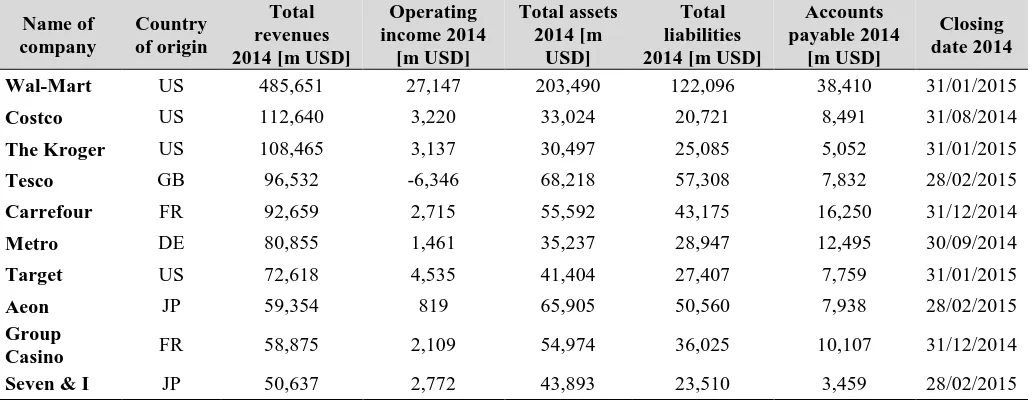
[image:5.595.42.558.486.687.2]Although several studies indicate that trade credits are one of the most important means of short term financing for companies (Summers and Wilson (2002), for example, state that more than 80% of business-to-business transactions in the UK include trade credit agreements), the amount of trade credit financing varies significantly from industry to industry (see Ng et al., 1999 or Seifert et al., 2013). The retail sector, which covers all types of companies selling goods or commodities bought from a manufacturer or a wholesaler to the end-user via different distribution channels, is an intensely cash-generating industry that relied extensively on trade credits in the past (see Klapper et al., 2012). Table 1 gives an overview of the operating characteristics of the world’s ten largest public-owned non-specialized retailers in terms of total revenues in 2014. In the considered sample, accounts payable reached on average one fifth of the firms’ total assets and one third of the firms’ total liabilities. At the individual company level, the world’s leading retailer, Wal-Mart Stores Inc., already had accounts payable of $38.410 billion in its balance sheet on January 31, 2015. This is about 85% of its total inventories ($45.141 billion). Even higher payables to inventory ratios can be found in the other companies that range from 88% (The Kroger Co. or Target Corporation) to 215% (Carrefour S.A.). Even though the demand for trade credit depends on several factors such as transaction pooling, credit rationing or financial flexibility in vendor-buyer relations (cf. Section 1 and Summers and Wilson, 2002, among others), reduced transaction cost as well as increased demand for liquidity after the economic downturn in the year 2008 seem to be the decisive causes of the high demand for trade credit in the retail sector.
Table 1: Top-10 global retailers according to total revenues in 2014
Name of company
Country of origin
Total revenues 2014 [m USD]
Operating income 2014
[m USD]
Total assets 2014 [m
USD]
Total liabilities 2014 [m USD]
Accounts payable 2014
[m USD]
Closing date 2014
Wal-Mart US 485,651 27,147 203,490 122,096 38,410 31/01/2015
Costco US 112,640 3,220 33,024 20,721 8,491 31/08/2014
The Kroger US 108,465 3,137 30,497 25,085 5,052 31/01/2015
Tesco GB 96,532 -6,346 68,218 57,308 7,832 28/02/2015
Carrefour FR 92,659 2,715 55,592 43,175 16,250 31/12/2014
Metro DE 80,855 1,461 35,237 28,947 12,495 30/09/2014
Target US 72,618 4,535 41,404 27,407 7,759 31/01/2015
Aeon JP 59,354 819 65,905 50,560 7,938 28/02/2015
Group
Casino FR 58,875 2,109 54,974 36,025 10,107 31/12/2014 Seven & I JP 50,637 2,772 43,893 23,510 3,459 28/02/2015 * other currencies have been converted to USD by the exchange rate at closing date
5 the buyer. In contrast, empirical studies indicate that even though the average effective interest rate of trade credits is high, the effective interest rates vary from a low of 2% to a high of 100% (Klapper et al., 2012). Consequently, in practice, the credit interest rate of the buyer, which could represent the interest rate the buyer could realize by depositing money in an interest bearing account or by investing it elsewhere, could also exceed the interest rate charged by the supplier. In such a case, it would not be rational from the buyer’s point of view to settle the unpaid balance immediately, as was assumed in the literature so far, but instead to keep the sales revenue invested and to settle the unpaid balance not before the interest charged by the supplier exceeds the incomes from the investment, or just before the next order is issued. Consequently, as long as the interest charged by the supplier on the open account is below the internal rate of return or the interest rates on short term deposits, the buyer may realize arbitrage profits from postponing the payment and investing the money in other projects or a bank account. Thus, the buyer has a financial incentive to extend the trade credit period, which also affects the average number of days payables outstanding and finally the effective cash conversion cycles.
Table 2: Days payables outstanding and cash conversion cycles of the retailers
Year
2005 2006 2007 2008 2009 2010 2011 2012 2013 2014 AV Company
DPO Wal-Mart 39 40 40 35 37 40 41 40 39 39 39
Costco 33 32 33 30 32 32 31 31 32 32 32
The Kroger 28 28 26 24 24 24 22 21 23 22 24
Tesco 29 31 34 35 37 39 38 38 36 32 35
Carrefour 102 99 96 93 91 96 92 78 78 82 91
Metro 93 101 104 98 103 102 103 96 100 75 97
Target 66 59 57 52 54 48 48 47 54 55 54
Aeon 65 64 65 66 74 73 72 65 69 80 69
Group Casino 84 74 79 70 72 73 70 70 64 66 72
Seven & I 28 22 21 19 34 32 39 39 40 40 32
CCC Wal-Mart 14 10 10 10 6 8 9 11 13 12 10
Costco 1 3 2 2 3 1 3 2 3 2 2
The Kroger 12 10 11 11 11 8 8 7 8 7 9
Tesco -6 -4 -3 -3 -5 -4 0 0 -2 -2 -3
Carrefour -57 -58 -54 -52 -51 -51 -45 -38 -38 -39 -48
Metro -38 -44 -47 -46 -48 -46 -45 -44 -36 -27 -42
Target 35 35 47 48 44 46 43 39 37 35 41
Aeon -9 -3 -4 -9 -16 -12 -8 5 23 19 -1
Group Casino -17 -13 -11 -8 -9 -7 -6 -5 -10 2 -8
6 Table 2 provides an overview of working capital measures of the retailers listed in Table 1, which gives some insights into the payment behaviors in the retail industry (note that Table 2 displays annual values based on each company`s fiscal year). A common measure for working capital management is the Cash Conversion Cycle (CCC) (cf. Richards and Laughlin, 1980) that measures the length of time (in days) a company’s cash is tied up in working capital. CCC is commonly calculated as the days of inventory outstanding (DIO) + the days accounts receivable outstanding (DRO) – the days accounts payable outstanding (DPO). To analyze the working capital management of the retailers, the CCC and its components were calculated for the years 2005 to 2014. The results show that there is a substantial difference between the ten retailers. Whereas some companies such as Wal-Mart Stores Inc. or The Kroger Co. exhibit a positive CCC in the past ten years, it is notably negative for others such as Carrefour S.A. or Metro AG. Regarding CCC’s components, the DIOs vary between a low of 19 days and a high of 59 days, while the DROs and DPOs vary between 3 and 36 days as well as 24 and 97 days, respectively. To gain further insights into this aspect, a cluster analysis of the retailers with regard to their DIO, DRO and DPO characteristics was performed with the help of the 𝑘-means approach. In the 𝑘-means analysis, an input data set is partitioned into k clusters by computing the squared distances between the inputs and the centroids and by assigning these inputs to the nearest centroid to minimize the consequent mean-squared error (cf. Rizman Zalik, 2008). The results show that companies with a positive CCC show a weighted average DIO of 30 days, a weighted average DRO of 5 days and a weighted average DPO of 31 days. In contrast, companies with a negative CCC have extended inventory cycles (DIO 43 days), but also significantly higher payment cycles for inbound and outbound transactions (DRO of 19 days and DPO of 74 days). Obviously, in the second cluster, companies have DPOs of more than two months. As large companies such as the retailers in our sample are supposed to have easy access to other sources of finance, they would not use trade credits extensively if it was as expensive as commonly hypothesized in the literature (cf. Ng et al., 1999, Klapper et al., 2012). Accordingly, beside other causes for the distinct payment behavior discussed in the literature, it is reasonable that due to the large varieties in contract conditions, trade credits appear comparatively cheap for some of the retailers in comparison with the return on alternative investment opportunities (we note that also power relationships cloud play an important role in this context which is, however, not reflected in our sample). This also seems to be supported by the fact that especially larger and investment-grade buyers receive longer net days from their suppliers (cf. Klapper et al., 2012). Hence, with an increasing interest rate, the retailers might realize arbitrage profits from postponing the payment to their suppliers, and therefore they tend to settle their payables outstanding later. To investigate this issue, which has been neglected in the literature so far, in more detail, the influence of financial conditions on the replenishment and payment behavior will be analyzed formally in the following. The results derived from this formal analysis may facilitate further empirical research.
Model development
The problem described in the introduction will subsequently be analyzed under the following conditions:
1. The inventory system involves a single item and has an infinite planning horizon. 2. Shortages are not allowed and the demand rate is constant and deterministic. 3. Lead time is zero and replenishments are made instantaneously.
7 case the buyer pays after time N, the supplier charges interest at the rate of Ic2, with Ic2 >
Ic1.
5. Apart from trade credits, the buyer is also assumed to have access to bank loans at the rate of Ib that are frequently referred to as substitutes to trade credits and vice versa.
6. The buyer has the option to deposit money in an interest bearing account with a fixed interest rate of Ie. Thus, s/he may use sales revenues to earn interest until the account is completely settled. Other investment decisions that are not related to the lot sizing problem are not considered.
In addition, the following terminology is used throughout the paper:
Parameters:
A cost of placing an order
C unit purchasing cost with C < P D demand rate per unit of time
h physical unit holding cost per unit and unit of time
Ic1 interest rate per unit of time charged by the supplier between times M and N Ic2 interest rate per unit of time charged by the supplier after time N
Ib interest rate on borrowings at the retailer per unit of time
Ie interest rate on deposits at the retailer per unit of time
M permissible delay in payments without any interest charge
N permissible delay in payments which induces an increase in the interest rate with N >
M
P selling price per unit
Decision variables
Q order quantity of the buyer (can implicitly be derived from 𝑇)
T replenishment interval
The buyer faces a constant customer demand rate D that leads to a continuous decrease in the inventory level I(t). Accordingly, the development of the inventory level with respect to time t
can be described by the following differential equation:
𝑑𝐼(𝑡)
𝑑𝑡 = −𝐷, 0 ≤ 𝑡 ≤ 𝑇 (1)
with the boundary conditions 𝐼(0) = 𝑄 and 𝐼(𝑇) = 0. The solution of this differential equation is:
𝐼(𝑡) = 𝐷(𝑇 − 𝑡), 0 ≤ 𝑡 ≤ 𝑇 (2)
which leads to the corresponding order quantity 𝑄 = 𝐷𝑇.
The total relevant costs are given as the sum of ordering, inventory carrying and interest costs, reduced by interest earnings. The cost per unit of time for placing an order at the supplier amounts to:
𝑂𝐶 = 𝐴 𝑇⁄ (3)
8
𝐼𝐻𝐶 =ℎ𝑇∫ 𝐼(𝑡)𝑑𝑡 =0𝑇 ℎ𝐷𝑇 2⁄ (4)
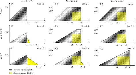
[image:9.595.76.549.166.428.2]Depending on the length of the replenishment cycle, 𝑇, the ratio of the interest rates (i.e. the ratio of 𝐼𝑒 to 𝐼𝑐1 and 𝐼𝑐2) and the lengths of the credit periods, M and N, the buyer may incur interest costs and/or realizes interest earnings.
Figure 1: Balance of accounts for deposits and liabilities
Figure 1 exemplarily illustrates the available amount of cash from sales revenues as well as the outstanding debt over time and thus facilitates determining interest cost and/or interest earnings (note that in Cases 1.2, 1.3 and 2.3, the spotted triangles representing continuous settlement of the outstanding debt depend on the ability of the retailer to settle the open account entirely at times M or N). Unless the interest rate on deposits (Ie) exceeds the interest charged by the supplier on the outstanding payments (Ic1) between times M and N, the buyer settles as much
of the account as possible at time M to avoid unnecessary interest cost (cf. left part of Figure 1). Depending on the length of the replenishment interval and the ability to settle the open account, three different cases with respective subcases may arise, namely 𝑇 ≤ 𝑀, 𝑀 < 𝑇 ≤ 𝑁 and 𝑇 > 𝑁 (see also Goyal et al., 2007). However, in case the interest rate on deposits (Ie) exceeds the debit interest rate (Ic1) between times M and N or even the debit interest (Ic2) after
9
Case 1: 𝐼𝑒 ≤ 𝐼𝑐1 < 𝐼𝑐2
Case 1.1: 𝑇 ≤ 𝑀
In this case, the buyer sells off the entire batch of 𝑄 = 𝐷𝑇 units at time T, and is able to settle the account completely before the supplier starts charging interest at time M. Between times 0 and T, sales revenues accumulate until the total revenue, PDT, is available at time T. During the period [0,M], the buyer additionally generates interest earnings at the rate Ie by depositing sales revenues in an interest bearing account. The total interest earned per unit of time can be written as:
𝐼𝐸1.1 =𝐼𝑒𝑃𝑇 [∫ 𝐷𝑡 𝑑𝑡0𝑇 + 𝑄(𝑀 − 𝑇)] = 𝐼𝑒𝑃𝐷 (𝑀 −𝑇2) (5)
To avoid interest payments to the supplier, the buyer settles the balance entirely at time M (i.e.
IC1.1= 0). Consequently, the total relevant costs amount to:
𝑇𝐶1.1 = 𝐴𝑇+ℎ𝐷𝑇2 − 𝐼𝑒𝑃𝐷 (𝑀 −𝑇2) (6)
Since the second-order condition of Eq. (6) is strictly positive (cf. Section 4), the solution can be derived using the first-order condition, which leads to the optimal value of T for Case 1.1:
𝑇1.1∗ = √ 2𝐴
𝐷(ℎ+𝐼𝑒 𝑃) (7)
Case 1.2: 𝑀 < 𝑇 ≤ 𝑁
In the case where Ie < Ic1 and M < TN, the buyer tries to settle as much of the unpaid balance
as possible at time M to minimize interest payments. In the period [0,M], the buyer sells DM
products and generates direct revenues in the amount of PDM dollars. Sales revenues that accumulate over time are deposited in an interest bearing account that earns interest at the rate of Ie per unit of time, which leads to additional earnings of 𝐼𝑒𝑃𝐷𝑀2⁄2 (cf. Eq. (8)). Accordingly, at time M, the buyer uses the sum of revenues and interest earnings to settle the open account. The total purchase cost for a lot of size DT amounts to CDT dollars. Depending on the ratio of the total purchase cost to the sum of earnings from sales and interest received at time M, two different subcases may arise that will be discussed in the following:
Case 1.2-1: 𝐶𝐷𝑇 ≤ 𝑃𝐷𝑀(1 + 𝐼𝑒𝑀 2⁄ )
In the first subcase, the sum of sales revenues and interest earned at time M is sufficient to settle the unpaid balance completely, i.e. 𝐶𝐷𝑇 ≤ 𝑃𝐷𝑀(1 + 𝐼𝑒𝑀 2⁄ ). The interest earnings per unit of time are given as:
𝐼𝐸1.2−1 =𝐼𝑒𝑃𝑇 ∫ 𝐷𝑡 𝑑𝑡0𝑀 = 𝐼𝑒𝑃𝐷𝑀 2
2𝑇 (8)
As the buyer again does not have to pay interest to the supplier in this subcase (i.e. IC2,1= 0), the total relevant costs amount to:
𝑇𝐶1.2−1 =𝐴𝑇+ℎ𝐷𝑇2 −𝐼𝑒𝑃𝐷𝑀 2
10 Since the second-order condition of Eq. (9) is strictly positive (cf. Section 4), the solution can be derived using of the first-order condition, which leads to the optimal value of T for Case 1.2-1:
𝑇1.2−1∗ = √2𝐴−𝐼𝑒𝑃𝐷𝑀 2
𝐷ℎ (10)
Case 1.2-2: 𝐶𝐷𝑇 > 𝑃𝐷𝑀(1 + 𝐼𝑒𝑀 2⁄ )
In contrast to the previous subcase, we now consider the case where the sum of sales revenues and interest earned at time M is not sufficient to settle the balance completely, i.e. 𝐶𝐷𝑇 >
𝑃𝐷𝑀(1 + 𝐼𝑒𝑀 2⁄ ). Thus, the supplier starts charging interest on the unpaid balance at the rate
Ic1 at time M. Interest earned in the period [0,M] is again given as 𝐼𝑒𝑃𝐷𝑀2⁄2 (cf. Eq. (8)),
which leads to an open account at time M in the amount of 𝐶𝐷𝑇 − 𝑃𝐷𝑀(1 + 𝐼𝑒𝑀 2⁄ ). To minimize interest payments, the buyer transfers each dollar earned after time M directly to the supplier (see Goyal et al., 2007 and Taleizadeh, 2014a; 2014b for a similar assumption in the case of trade credits or prepayments). For the case where the unpaid balance cannot be settled at time M, but before time N, the interest cost can be formulated as follows:
𝐼𝐶1.2−2 =𝐼𝑐𝑇1∫𝑀𝑀+𝑧1((𝐶𝐷𝑇 − 𝑃𝐷𝑀(1 + 𝐼𝑒𝑀 2⁄ )) − 𝑃𝐷(𝑡 − 𝑀)) 𝑑𝑡 =2𝑃𝐷𝑇𝐼𝑐1 (𝐶𝐷𝑇 −
𝑃𝐷𝑀(1 + 𝐼𝑒𝑀 2⁄ ))2 (11)
where 𝑀 + 𝑧1 denotes the point in time when the unpaid balance has been completely settled, with 𝑧1 = (𝐶𝐷𝑇 − 𝑃𝐷𝑀(1 + 𝐼𝑒𝑀 2⁄ ))/𝑃𝐷. In case of 𝐼𝑏 < 𝐼𝑐1 < 𝐼𝑐2, the retailer may benefit from bridgeover finance by bank loans that reduce the effective interest rate (note that in this case in Eq. (11), 𝐼𝑐1 needs to be replaced by Ib; everything else would remain unchanged). Thus, the total costs for this case amount to:
𝑇𝐶1.2−2 =𝐴𝑇+ℎ𝐷𝑇2 +2𝑃𝐷𝑇𝐼𝑐1 (𝐶𝐷𝑇 − 𝑃𝐷𝑀(1 + 𝐼𝑒𝑀 2⁄ ))2−𝐼𝑒𝑃𝐷𝑀 2
2𝑇 (12)
Since the second-order condition of Eq. (12) is strictly positive (cf. Section 4), the solution can be derived using the first-order condition, which leads to the optimal value of T for Case 1.2-1:
𝑇1.2−2∗ = √2𝐴+𝑃𝐷𝑀2(𝐼𝑐1(1+𝐼𝑒𝑀 2⁄ )2−𝐼𝑒)
𝐷(ℎ+𝐼𝑐1𝐶2⁄ )𝑃 (13)
Case 1.3: 𝑁 < 𝑇
The case where Ie < Ic1 and T > N is similar to Case 1.2. Again, the buyer uses the revenues
and interest earned to pay the supplier. To minimize interest payments, he/she settles as much of the outstanding balance as possible at time M and afterwards reduces the outstanding amount continuously by transferring each dollar of the sales revenues to the supplier’s account. This helps to avoid unnecessary interest costs as compared to prior works in this area assuming that partial payments are made at times M and N only. In addition, interest charges that accrue between times M and N will be considered, which leads to an unsettled balance at time N in the amount of 𝐶𝐷𝑇 − 𝑃𝐷𝑀(1 + 𝐼𝑒𝑀 2⁄ ) − 𝑃𝐷(𝑁 − 𝑀) + 𝐼𝑐1∫ ((𝐶𝐷𝑇 − 𝑃𝐷𝑀(1 +𝑀𝑁
11 expression leads to (𝐶𝐷𝑇 − 𝑃𝐷𝑀(1 + 𝐼𝑒𝑀 2⁄ ))(1 + 𝐼𝑐1(𝑁 − 𝑀)) − 𝑃𝐷(𝑁 − 𝑀)(1 +
𝐼𝑐1(𝑁 − 𝑀) 2⁄ ). The first part of this expression describes the outstanding balance at time M, which includes interest incurred at the rate Ic1. The second part of the expression, in contrast,
represents the amount of repayment during times M and N, which also considers the interest effect due to the continuous refund.
In contrast to prior works on trade credits with progressive credit periods, these modifications allow us to consider the interest charges that accumulate between times M and N as well as the payments the buyer makes between times M and N to reduce the accruing interest. According to the ratio of the total purchasing cost to the sum of sales and interest earnings, three possible subcases may arise that can be distinguished based on the balance of the buyer’s account at times M and N, respectively.
Case 1.3-1: 𝐶𝐷𝑇 ≤ 𝑃𝐷𝑀(1 + 𝐼𝑒𝑀 2⁄ )
The case where Ie < Ic1 and T > N is identical to Subcase 1.2-1. Thus, the buyer settles the
account completely at time M without paying any interest charges to the supplier.
Case 1.3-2: 𝐶𝐷𝑇 > 𝑃𝐷𝑀(1 + 𝐼𝑒𝑀 2⁄ ) and (𝐶𝐷𝑇 − 𝑃𝐷𝑀(1 + 𝐼𝑒𝑀 2⁄ ))(1 + 𝐼𝑐1(𝑁 −
𝑀)) ≤ 𝑃𝐷(𝑁 − 𝑀)(1 + 𝐼𝑐1(𝑁 − 𝑀) 2⁄ )
The case where Ie < Ic1 and T > N is identical to Subcase 1.2-2. Thus, the buyer is not able to
pay off the entire purchase cost at time M, but settles as much of the account as possible at time
M. Afterwards, he/she continuously reduces the open account by transferring sales revenues to the supplier. The account is settled at time 𝑀 + 𝑧1 with 𝑀 + 𝑧1 < 𝑁, and the supplier charges an interest on the unpaid balance between times M and 𝑀 + 𝑧1.
Case 1.3-3: 𝐶𝐷𝑇 > 𝑃𝐷𝑀(1 + 𝐼𝑒𝑀 2⁄ ) and (𝐶𝐷𝑇 − 𝑃𝐷𝑀(1 + 𝐼𝑒𝑀 2⁄ ))(1 + 𝐼𝑐1(𝑁 −
𝑀)) > 𝑃𝐷(𝑁 − 𝑀)(1 + 𝐼𝑐1(𝑁 − 𝑀) 2⁄ )
In the case where Ie < Ic1 and T > N, the buyer is not able to pay off the total purchase cost at
times M or N. Thus, he/she settles as much of the unpaid balance as possible at time M. Afterwards, the open account is continuously reduced by transferring each dollar earned from sales to the supplier. As the buyer has no incentive to authorize any payments before time M, he/she realizes interest earnings in the period [0,M] (cf. Eq. (8)). The supplier, in turn, charges interest on the gradually decreasing unpaid balance at the rate Ic1 between times M and N and
at the rate Ic2 after time N.
Hence, the overall interest cost per unit of time for this case, IC1.3-3, amounts to:
𝐼𝐶1.3−3 =𝐼𝑐1
𝑇 ∫ ((𝐶𝐷𝑇 − 𝑃𝐷𝑀 (1 +
𝐼𝑒𝑀
2 )) − 𝑃𝐷(𝑡 − 𝑀)) 𝑑𝑡 𝑁
𝑀 +
𝐼𝑐2
𝑇 ∫ ((𝐶𝐷𝑇 −
𝑁+𝑧2 𝑁
𝑃𝐷𝑀 (1 +𝐼𝑒𝑀2 )) (1 + 𝐼𝑐1(𝑁 − 𝑀)) − 𝑃𝐷(𝑁 − 𝑀) (1 +𝐼𝑐1(𝑁−𝑀)2 ) − 𝑃𝐷(𝑡 − 𝑁)) 𝑑𝑡 =
𝐼𝑐1(𝑁−𝑀)
𝑇 (𝐶𝐷𝑇 − 𝑃𝐷𝑀 (1 +
𝐼𝑒𝑀
2 ) −
𝑃𝐷(𝑁−𝑀)
2 ) +
𝐼𝑐2
2𝑃𝐷𝑇((𝐶𝐷𝑇 − 𝑃𝐷𝑀 (1 +
𝐼𝑒𝑀
2 )) (1 +
𝐼𝑐1(𝑁 − 𝑀)) − 𝑃𝐷(𝑁 − 𝑀) (1 +𝐼𝑐1(𝑁−𝑀)2 )) 2
12
𝐼𝑐1𝑃𝐷(𝑁 − 𝑀)2⁄ ) /𝑃𝐷2 . In case of 𝐼𝑏 < 𝐼𝑐
1 < 𝐼𝑐2 or 𝐼𝑐1 < 𝐼𝑏 < 𝐼𝑐2, the retailer may
benefit from bridgeover finance by bank loans that reduce the effective interest rate (note that in this case in Eq.(14) 𝐼𝑐1 and /or 𝐼𝑐2 need to be replaced by Ib; everything else would remain
unchanged). The total cost for this case amounts to:
𝑇𝐶1.3−3 =𝐴𝑇+ℎ𝐷𝑇2 +𝐼𝑐1(𝑁−𝑀)𝑇 (𝐶𝐷𝑇 − 𝑃𝐷𝑀 (1 +𝐼𝑒𝑀2 ) −𝑃𝐷(𝑁−𝑀)2 ) + 𝐼𝑐2
2𝑃𝐷𝑇((𝐶𝐷𝑇 −
𝑃𝐷𝑀 (1 +𝐼𝑒𝑀2 )) (1 + 𝐼𝑐1(𝑁 − 𝑀)) − 𝑃𝐷(𝑁 − 𝑀) (1 +𝐼𝑐1(𝑁−𝑀)
2 ))
2
−𝐼𝑒𝑃𝐷𝑀2𝑇 2 (15)
Since the second-order condition of Eq. (15) is strictly positive (cf. Section 4), the solution can be derived using the first-order condition, which leads to the optimal value of T for Case 1.3-3:
𝑇1.3−3∗ =
√2𝐴+𝐼𝑐2𝑃𝐷(𝑀(1+𝐼𝑐1(𝑁−𝑀))(1+𝐼𝑐1(𝑁−𝑀)2 )+(𝑁−𝑀)(1+ 𝐼𝑒𝑀
2 ))
2
−2𝐼𝑐1(𝑁−𝑀)(𝑃𝐷𝑀(1+𝐼𝑒𝑀2 )+𝑃𝐷(𝑁−𝑀)2 )−𝐼𝑒𝑃𝐷𝑀2
𝐷(ℎ+𝐼𝑐2𝐶2𝑃(1+𝐼𝑐1(𝑁−𝑀))2)
(16) After some algebraic manipulations, the buyer’s total cost function for the interest structure
𝐼𝑒 < 𝐼𝑐1 < 𝐼𝑐2 (Case 1) may be summarized as follows:
𝑇𝐶1 = 𝐴𝑇+ℎ𝐷𝑇2 +2𝑃𝐷𝑇𝐼𝑐1 [(𝑚𝑎𝑥 {𝐶𝐷𝑇 − 𝑃𝐷𝑀 (1 +𝐼𝑒𝑀2 ) , 0}) 2
− (𝑚𝑎𝑥 {𝐶𝐷𝑇 − 𝑃𝐷𝑀 (1 +
𝐼𝑒𝑀
2 ) − 𝑃𝐷(𝑁 − 𝑀), 0}) 2
] + 𝐼𝑐2
2𝑃𝐷𝑇[(𝑚𝑎𝑥 {(𝐶𝐷𝑇 − 𝑃𝐷𝑀 (1 +
𝐼𝑒𝑀
2 )) (1 + 𝐼𝑐1(𝑁 − 𝑀)) −
𝑃𝐷(𝑁 − 𝑀) (1 +𝐼𝑐1(𝑁−𝑀)2 ) , 0})2] −𝐼𝑒𝑃𝐷2𝑇 [𝑀2 − (𝑚𝑎𝑥{𝑀 − 𝑇, 0})2] (17)
Case 2: 𝐼𝑐1 < 𝐼𝑒 ≤ 𝐼𝑐2
Case 2.1: 𝑇 ≤ 𝑀
For Ie > Ic1 andT M, the buyer may benefit from keeping the sales revenue in an interest
bearing account until time N and from settling the account after this point in time. Between times M and N, he/she has to pay interest to the supplier. However, since Ie > Ic1, the interest
earned exceeds the interest paid during this period. Similar to Subcase 1.1 (cf. Eq. (5)), the interest earned per unit of time can be calculated as:
𝐼𝐸2.1 = 𝐼𝑒𝑃𝑇 [∫ 𝐷𝑡 𝑑𝑡0𝑇 + 𝑄(𝑁 − 𝑇)] = 𝐼𝑒𝑃𝐷 (𝑁 −𝑇2) (18)
The overall interest cost between times M and N amounts to:
𝐼𝐶2.1 =𝐼𝑐𝑇1𝐶𝑄(𝑁 − 𝑀) (19)
13
𝑇𝐶2.1 =𝐴𝑇+ℎ𝐷𝑇2 +𝐼𝑐𝑇1𝐶𝑄(𝑁 − 𝑀) − 𝐼𝑒𝑃𝐷 (𝑁 −𝑇2) (20)
Since the second-order condition of Eq. (21) is strictly positive (cf. Section 4), the solution can be derived using the first-order condition, which leads to the optimal value of T for Case 2.1:
𝑇2.1∗ = √ 2𝐴
𝐷(ℎ+𝐼𝑒𝑃) (21)
Case 2.2: 𝑀 < 𝑇 ≤ 𝑁
The case where M < T < N and Ic1 < Ie is identical to Case 2.1. In this case, the buyer accepts
interest charges between times M and N caused by the postponement of the payment and realizes interest earnings by depositing sales revenues in an interest bearing account. The account is completely settled at time N.
Case 2.3: 𝑁 < 𝑇
In the case where Ic1 < Ie and N < T, as much of the unpaid balance is settled at time N as
possible to minimize interest payments. In the period [0,N], the buyer sells a total quantity of
DN units and generates direct sales revenues in the amount of PDN dollars. Sales revenues that accumulate over time are deposited in an interest bearing account that earns interest at the rate of Ie per unit of time, which leads to additional earnings of 𝐼𝑒𝑃𝐷𝑁2⁄2 (cf. Eq. (23)). Thus, at time N, the buyer uses the sum of sales revenues and interest earnings to settle the open account. The total purchase cost for a lot of size DT again amounts to CDT dollars. According to the ratio of the total purchase cost and the accruing interest to the total sales revenues and interest earnings at time N, two possible subcases may arise that will be discussed in the following:
Case 2.3-1: 𝐶𝐷𝑇(1 + 𝐼𝑐1(𝑁 − 𝑀)) ≤ 𝑃𝐷𝑁(1 + 𝐼𝑒𝑁 2⁄ )
If the interest rate of the buyer, Ie, exceeds the interest charges of the supplier for the first credit period, Ic1, he/she will again not settle the account before time N. Instead, the buyer keeps the sales revenues earned in period [M,N] in an interest bearing account. As the account is completely settled at time N, the interest earned per unit of time is given as:
𝐼𝐸2.3−1 =𝐼𝑒𝑃𝑇 ∫ 𝐷𝑡 𝑑𝑡0𝑁 = 𝐼𝑒𝑃𝐷𝑁2𝑇 2 (22)
The interest charges in this case are the same as those derived for Case 2.1 (cf. Eq. (20)). Thus, the total costs can be formulated as:
𝑇𝐶2.3−1= 𝐴𝑇+ℎ𝐷𝑇2 +𝐼𝑐1
𝑇 𝐶𝑄(𝑁 − 𝑀) −
𝐼𝑒𝑃𝐷𝑁2
2𝑇 (23)
Since the second-order condition of Eq. (24) is strictly positive (cf. Section 4), the solution can be derived using the first-order condition, which leads to the optimal value of T for Case 2.3-1:
𝑇2.3−1∗ = √2𝐴−𝐼𝑒𝑃𝐷𝑁2
ℎ𝐷 (24)
14 For the case where Ie > Ic1 and where the buyer is unable to pay off the total purchase cost at
time N, the account is partially settled at time N. Afterwards, the unpaid balance is continuously reduced by transferring each dollar earned to the supplier’s account until the balance has been completely settled. The interest earned in the period [0,N] is given as 𝐼𝑒𝑃𝐷𝑁2⁄2 (cf. Eq. (23)), which again considers the interest advantage that results from accruing interest earnings due to the delayed payment. The supplier, however, charges interest on the gradually decreasing unpaid balance at the rate Ic2 after time N which is given as:
𝐼𝐶2.3−2= 𝐼𝑐1
𝑇 𝐶𝑄(𝑁 − 𝑀) +
𝐼𝑐2
𝑇 ∫ ((𝐶𝐷𝑇(1 + 𝐼𝑐1(𝑁 − 𝑀)) − 𝑃𝐷𝑁(1 + 𝐼𝑒𝑁 2⁄ )) −
𝑁+𝑧3 𝑁
𝑃𝐷(𝑡 − 𝑁)) 𝑑𝑡 =𝐼𝑐1
𝑇 𝐶𝑄(𝑁 − 𝑀) +
𝐼𝑐2
2𝑇𝑃𝐷[𝐶𝑄(1 + 𝐼𝑐1(𝑁 − 𝑀)) − 𝑃𝐷𝑁(1 + 𝐼𝑒𝑁 2⁄ )] 2
(25)
where N+z3 denotes the point in time when the unpaid balance has been completely settled,
with 𝑧3 = (𝐶𝐷𝑇(1 + 𝐼𝑐1(𝑁 − 𝑀)) − 𝑃𝐷𝑁(1 + 𝐼𝑒𝑁 2⁄ )) /𝑃𝐷. In case of 𝐼𝑐1 < 𝐼𝑏 < 𝐼𝑐2, the retailer may benefit from bridgeover finance by bank loans that reduce the effective interest rate (note that in this case in Eq.(25) 𝐼𝑐2 needs to be replaced by Ib; everything else would remain unchanged). The total costs for this case amount to:
𝑇𝐶2.3−2= 𝐴𝑇+ℎ𝐷𝑇2 +𝐼𝑐𝑇1𝐶𝑄(𝑁 − 𝑀) +2𝑃𝐷𝑇𝐼𝑐2 (𝐶𝐷𝑇(1 + 𝐼𝑐1(𝑁 − 𝑀)) − 𝑃𝐷𝑁(1 +
𝐼𝑒𝑁 2⁄ ))2−
𝐼𝑒𝑃𝐷𝑁2 2𝑇
(26)
Since the second-order condition of Eq. (27) is strictly positive (cf. Section 4), the solution can be derived using the first-order condition, which leads to the optimal value of T for Case 2.3-1:
𝑇2.3−2∗ = √2𝐴+𝑃𝐷𝑁2(𝐼𝑐2(1+𝐼𝑒𝑁 2⁄ )2−𝐼𝑒) 𝐷
𝑃
⁄ (ℎ𝑃+𝐼𝑐2𝐶2(1+𝐼𝑐1(𝑁−𝑀))2) (27)
After some algebraic manipulations, the buyer’s total cost function for the interest structure
𝐼𝑐1 < 𝐼𝑒 < 𝐼𝑐2 (Case 2) can be summarized as follows:
𝑇𝐶2 =𝐴𝑇+ℎ𝐷𝑇2 +𝐼𝑐𝑇1𝐶𝑄(𝑁 − 𝑀) +2𝑃𝐷𝑇𝐼𝑐2 [(𝑚𝑎𝑥 {(𝐶𝐷𝑇(1 + 𝐼𝑐1(𝑁 − 𝑀)) − (𝑃𝐷𝑁 +
𝐼𝑒𝑃𝐷𝑁2⁄ )) , 0})2 2] −𝐼𝑒𝑃𝐷
2𝑇 [𝑁
2− (𝑚𝑎𝑥{𝑁 − 𝑇, 0})2] (28)
Case 3: 𝐼𝑐1 < 𝐼𝑐2 < 𝐼𝑒
Case 3.1: 𝑇 ≤ 𝑀
Since Ie > Ic2, the retailer again has an incentive to postpone the payment or even to never pay
15 default credit, it is reasonable to assume that the buyer has to settle the open account at the end of the last credit period. Thus, for Ie > Ic2 andTM, the buyer may again benefit from keeping
the sales revenue in an interest bearing account until time N. Between times M and N, he/she has to pay interest to the supplier that will, however, be offset by the interest earnings in this period. As for Subcase 2.1 (cf. Eq. (20)), the total costs are given as:
𝑇𝐶3.1 =𝐴𝑇+ℎ𝐷𝑇2 +𝐼𝑐1
𝑇 𝐶𝑄(𝑁 − 𝑀) − 𝐼𝑒𝑃𝐷 (𝑁 −
𝑇
2) (29)
Since the second-order condition of Eq. (29) is strictly positive (cf. Section 4), the solution can be derived using the first-order condition, which leads to the optimal value of T for Case 3.1:
𝑇3.1∗ = √ 2𝐴
𝐷(ℎ+𝐼𝑒𝑃) (30)
Case 3.2: 𝑀 < 𝑇 ≤ 𝑁
The case where M < T < N and Ic2 < Ie is identical to Case 3.1. Again, the buyer accepts interest
charges between times M and N that result from postponing the payment to the supplier, and he/she thus realizes interest earnings by depositing sales revenues in an interest bearing account. The account is completely settled at time N.
Case 3.3: 𝑁 < 𝑇
In the case where Ic2 < Ie and N < T, the buyer may benefit from postponing the payment as
long as possible and could also benefit from never settling the open account. We may, however, assume that the supplier would not be willing to offer a credit with infinite duration. As the trade credit serves the purpose to influence the buyer’s ordering behavior on a per-order bases, we may assume that the buyer has to settle the open account at time T, right before the next order is issued (and right before the next trade credit is granted). In the period [0,T], the buyer sells off the entire lot of DT units and generates direct sales revenues in the amount of PDT
dollars. In addition, sales revenues that accumulate over time are deposited in an interest bearing account that earns interest at the rate of Ie per unit of time, which leads to additional earnings of:
𝐼𝐸3.3 = 𝐼𝑒𝑃𝑇 ∫ 𝐷𝑡 𝑑𝑡0𝑇 =𝐼𝑒𝑃𝐷𝑇2 (31)
At time T, the buyer uses sales revenues and interest earnings to settle the total purchase cost of CDT dollars as well as the accruing interest charges between times M and T. The interest cost amounts to:
𝐼𝐶3.3 =𝐼𝑐𝑇1𝐶𝑄(𝑁 − 𝑀) +𝐼𝑐𝑇2𝐶𝑄(𝑇 − 𝑁)(1 + 𝐼𝑐1(𝑁 − 𝑀)) (32)
Consequently, the total costs can be formulated as:
𝑇𝐶3.3 =𝐴𝑇+ℎ𝐷𝑇2 +𝐼𝑐𝑇1𝐶𝑄(𝑁 − 𝑀) +𝐼𝑐𝑇2𝐶𝑄(𝑇 − 𝑁)(1 + 𝐼𝑐1(𝑁 − 𝑀)) −𝐼𝑒𝑃𝐷𝑇2 (33)
16
𝑇3.3∗ = √ 2𝐴
𝐷(ℎ+2𝐼𝑐2𝐶(1+𝐼𝑐1(𝑁−𝑀))−𝐼𝑒𝑃) (34)
After some algebraic manipulations, the buyer’s total cost function for the interest structure
𝐼𝑐1 < 𝐼𝑐2 < 𝐼𝑒 (Case 3) can be summarized as follows:
𝑇𝐶3 =𝐴𝑇+ℎ𝐷𝑇2 +𝐼𝑐𝑇1𝐶𝐷𝑇(𝑁 − 𝑀) +𝐼𝑐𝑇2𝐶𝐷𝑇(1 + 𝐼𝑐1(𝑁 − 𝑀))𝑚𝑎𝑥 {𝑇 − 𝑁, 0} − 𝐼𝑒𝑃𝐷 (𝑇2+
𝑚𝑎𝑥{𝑁 − 𝑇, 0}) (35)
A summery table with closed form solutions as well as the corresponding optimality conditions for all relevant cases can be found in the online supplement.
Solution approach
For convenience, we assume that all 𝑇𝐶𝑖(𝑇) with 𝑖 representing the respective case (𝑖 =
{1.1,1.2 − 1, . . . }) are defined on 𝑇 > 0. To find the optimal solution for the problem presented above, all 𝑇𝐶𝑖(𝑇) are minimized separately and compared with regard to their range of validity to obtain an optimal value of T.
In Case 1.1, the first-order condition for a minimum is:
𝑑TC1.1
𝑑𝑇 = −
𝐴 𝑇2+
ℎ𝐷
2 +
Ie𝑃𝐷
2 = 0 (36)
Theorem 1. Let 𝑇 = 𝑇1.1∗ be the solution of (36). (a) Eq. (36) has a unique solution.
(b) If 𝑇1.1 ≤ 𝑀, then 𝑇1.1∗ is the global minimum of 𝑇𝐶1.1.
Proof: See Appendix A.
In Case 1.2-1, the first-order condition for a minimum is:
𝑑TC1.2−1
𝑑𝑇 =−
𝐴 𝑇2+
ℎ𝐷
2 +
𝐼𝑒𝑃𝐷𝑀2
2𝑇2 = 0 (37)
Theorem 2. Let 𝑇 = 𝑇1.2−1∗ be the solution of (37). (a) Eq. (37) has a unique solution.
(b) If 𝑀 < 𝑇1.2−1 ≤ 𝑁 and 𝐶𝐷𝑇1.2−1 ≤ 𝑃𝐷𝑀(1 + 𝐼𝑒𝑀 2⁄ ), then 𝑇1.2−1∗ is the global
minimum of 𝑇𝐶1.2−1.
Proof: See Appendix B.
In Case 1.2-2, the first-order condition for a minimum is:
𝑑𝑇𝐶1.2−2
𝑑𝑇 = −
𝐴 𝑇2+
ℎ𝐷
2 +
𝐼𝑐1𝐷𝐶2
2𝑃 −
𝑃𝐷𝑀2
2𝑇2 (𝐼𝑐1(1 + 𝐼𝑒𝑀 2⁄ )
2− 𝐼𝑒)= 0 (38)
17 (a) Eq. (38) has a unique solution.
(b) If 𝑀 < 𝑇1.2−2 ≤ 𝑁 and 𝐶𝐷𝑇1.2−2 > 𝑃𝐷𝑀(1 + 𝐼𝑒𝑀 2⁄ ), then 𝑇1.2−2∗ is the global minimum of 𝑇𝐶1.2−2.
Proof: See Appendix C.
The total cost function in Case 1.3-1 is identical to Subcase 1.2-1. Accordingly, the theoretical analysis for this case is consequently the same than the one presented for Theorem 2.
Corollary 1. If 𝑁 < 𝑇1.3−1 and 𝐶𝐷𝑇1.3−1 ≤ 𝑃𝐷𝑀(1 + 𝐼𝑒𝑀 2⁄ ), then 𝑇1.3−1∗ is the global minimum of 𝑇𝐶1.3−1.
Proof:
If 𝑇 = 𝑇1.3−1∗ is the solution to 𝑑𝑇𝐶1.3−1⁄𝑑𝑇= 0, the second-order derivative of 𝑇𝐶1.3−1 at this point is:
𝑑2𝑇𝐶1.3−1(𝑇)
𝑑𝑇2 |𝑇
1.3−1∗
= √(ℎ𝐷)3⁄2𝐴 − 𝐼𝑒𝑃𝐷𝑀2 > 0.
Hence, 𝑇1.3−1∗ is the global minimum of 𝑇𝐶1.3−1. Additionally, by substituting 𝑇1.3−1∗ into 𝑁 <
𝑇 and 𝐶𝐷𝑇 ≤ 𝑃𝐷𝑀(1 + 𝐼𝑒𝑀 2⁄ ), we know that if and only if 𝐼𝑒𝑃𝐷𝑀2+ ℎ𝐷𝑁2 < 2𝐴 ≤
𝐷𝑀2(𝐼𝑒𝑃 + ℎ(𝑃 𝐶⁄ )2(1 + 𝐼𝑒𝑀 2⁄ )2) , then 𝑁 < 𝑇
1.3−1∗ and 𝐶𝐷𝑇1.3−1∗≤ 𝑃𝐷𝑀(1 +
𝐼𝑒𝑀 2⁄ ).
The total cost function in Case 1.3-2 is identical to Subcase 1.2-2. Accordingly, the theoretical analysis for this case is consequently the same than the one presented for Theorem 3.
Corollary 2. If 𝑁 < 𝑇1.3−2 , 𝐶𝐷𝑇1.3−2> 𝑃𝐷𝑀(1 + 𝐼𝑒𝑀 2⁄ ) and (𝐶𝐷𝑇1.3−2− 𝑃𝐷𝑀(1 +
𝐼𝑒𝑀 2⁄ ))(1 + 𝐼𝑐1(𝑁 − 𝑀)) ≤ 𝑃𝐷 2⁄ (2(𝑁 − 𝑀)−𝐼𝑐1(𝑁 − 𝑀)2), then 𝑇1.3−2∗ is the global
minimum of 𝑇𝐶1.3−2. Proof:
If 𝑇 = 𝑇1.3−2∗ is the solution to 𝑑𝑇𝐶1.3−2⁄𝑑𝑇= 0, the second-order derivative of 𝑇𝐶1.3−2 at this point is:
𝑑2𝑇𝐶1.3−2(𝑇)
𝑑𝑇2 |𝑇
1.3−2∗
= √(𝐷(ℎ + 𝐼𝑐1𝐶2⁄ ))𝑃 3 (2𝐴 + 𝑃𝐷𝑀2(𝐼𝑐
1(1 + 𝐼𝑒𝑀 2⁄ )2 − 𝐼𝑒))
⁄ > 0.
Hence, 𝑇1.3−2∗ is the global minimum of TC1.3−2. Additionally, by substituting 𝑇1.3−2∗ into 𝑁 <
𝑇 and 𝐶𝐷𝑇 ≤ 𝑃𝐷𝑀(1 + 𝐼𝑒𝑀 2⁄ ), we know that if and only if (ℎ + 𝐼𝑐1𝐶2⁄ )𝐷∆𝑃 22−
𝑃𝐷𝑀2(𝐼𝑐
1(1 + 𝐼𝑒𝑀 2⁄ )2− 𝐼𝑒) < 2𝐴 ≤ (ℎ + 𝐼𝑐1𝐶2⁄ )𝐷∆𝑃 32− 𝑃𝐷𝑀2(𝐼𝑐1(1 + 𝐼𝑒𝑀 2⁄ )2−
𝐼𝑒) with ∆2= 𝑚𝑎𝑥{𝑁, 𝑀(𝑃 𝐶⁄ )(1 + 𝐼𝑒𝑀 2⁄ )} and ∆3=
(𝑃(2(𝑁 − 𝑀)−𝐼𝑐1(𝑁 − 𝑀)2) 2𝐶(1 + 𝐼𝑐⁄ 1(𝑁 − 𝑀))+ 𝑀𝑃(1 + 𝐼𝑒𝑀 2⁄ ) 𝐶⁄ ) , then 𝑁 <
𝑇1.3−2∗ , 𝐶𝐷𝑇
1.3−2∗ ≤ 𝑃𝐷𝑀(1 + 𝐼𝑒𝑀 2⁄ ) and (𝐶𝐷𝑇1.3−2∗ − 𝑃𝐷𝑀(1 + 𝐼𝑒𝑀 2⁄ ))(1 + 𝐼𝑐1(𝑁 −
𝑀)) ≤ 𝑃𝐷 2⁄ (2(𝑁 − 𝑀)−𝐼𝑐1(𝑁 − 𝑀)2).
18
𝑑𝑇𝐶1.3−3
𝑑𝑇 = −
𝐴 𝑇2+
ℎ𝐷
2 +
𝐼𝑐1(𝑁−𝑀)
𝑇2 (𝑃𝐷𝑀(1 +
𝐼𝑒𝑀 2 )+
𝑃𝐷(𝑁−𝑀)
2 )+
𝐼𝑐2𝐷𝐶2
2𝑃 (1 + 𝐼𝑐1(𝑁 − 𝑀)) 2
−
𝐼𝑐2𝑃𝐷
2𝑇2 (𝑀(1 + 𝐼𝑐1(𝑁 − 𝑀)) (1 +
𝐼𝑐1(𝑁−𝑀)
2 )+(𝑁 − 𝑀) (1 + 𝐼𝑒𝑀
2 )) 2
+𝐼𝑒𝑃𝐷𝑀2
2𝑇2 = 0 (39) Theorem 4. Let 𝑇 = 𝑇1.3−3∗ be the solution of (39).
(a) Eq. (39) has a unique solution.
(b) If 𝑁 < 𝑇1.3−3 , 𝐶𝐷𝑇1.3−3> 𝑃𝐷𝑀(1 + 𝐼𝑒𝑀 2⁄ ) and (𝐶𝐷𝑇1.3−3− 𝑃𝐷𝑀(1 +
𝐼𝑒𝑀 2⁄ ))(1 + 𝐼𝑐1(𝑁 − 𝑀)) > 𝑃𝐷(𝑁 − 𝑀)(1 + 𝐼𝑐1(𝑁 − 𝑀) 2⁄ ), then 𝑇1.3−3∗ is the
global minimum of 𝑇𝐶1.3−3.
Proof: See Appendix D.
In Case 2.1, the first-order condition for a minimum is:
𝑑TC2.1
𝑑𝑇 = −
𝐴 𝑇2+
ℎ𝐷
2 +
𝐼𝑒𝑃𝐷
2 = 0 (40)
Theorem 5. Let 𝑇 = 𝑇2.1∗ be the solution of (40). (a) Eq. (40) has a unique solution.
(b) If 𝑇2.1 ≤ 𝑀, then 𝑇2.1∗ is the global minimum of 𝑇𝐶2.1.
Proof: The proof of this theorem is similar to the proof of Theorem 1 since Eq. (36) and Eq. (40) are identical.
The total cost function in Case 2.2 is identical to Case 2.1. The theoretical analysis for this case is consequently the same as the one presented for Theorem 1.
Corollary 3. If 𝑀 < 𝑇2.2 ≤ 𝑁, then 𝑇2.2∗ is the global minimum of 𝑇𝐶2.2.
Proof:
If 𝑇 = 𝑇2.2∗ is the solution to 𝑑𝑇𝐶2.2⁄𝑑𝑇= 0, the second-order derivative of 𝑇𝐶2.2 at this point is:
𝑑2𝑇𝐶
2.2(𝑇)
𝑑𝑇2 |𝑇 2.2∗
= √(𝐷(ℎ + 𝑃𝐼𝑒)3⁄2𝐴 > 0.
Hence, 𝑇2.2∗ is the global minimum of 𝑇𝐶2.2. Additionally, by substituting 𝑇2.2∗ into 𝑀 < 𝑇 ≤
𝑁, we know that if and only if (ℎ + 𝐼𝑒𝑃)𝐷𝑀2 < 2𝐴 ≤ (ℎ + 𝐼𝑒𝑃)𝐷𝑁2, then 𝑀 < 𝑇2.2∗ ≤ 𝑁. In Case 2.3-1, the first-order condition for a minimum is:
𝑑TC2.3−1
𝑑𝑇 =−
𝐴 𝑇2+
ℎ𝐷
2 +
𝐼𝑒𝑃𝐷𝑁2
2𝑇2 = 0 (41)
19 (b) If 𝑁 < 𝑇2.3−1 and 𝐶𝐷𝑇2.3−1(1 + 𝐼𝑐1(𝑁 − 𝑀)) ≤ 𝑃𝐷𝑁(1 + 𝐼𝑒𝑁 2⁄ ), then 𝑇2.3−1∗ is the
global minimum of 𝑇𝐶2.3−1.
Proof: See Appendix E.
In Case 2.3-2, the first-order condition for a minimum is:
𝑑TC2.3−2
𝑑𝑇 = −
𝐴 𝑇2−
𝑃𝐷𝑁2
2𝑇2 (𝐼𝑐2(1 + 𝐼𝑒𝑁 2⁄ )
2− 𝐼𝑒)+𝐷 2(ℎ +
𝐶2
𝑃 𝐼𝑐2(1 + 𝐼𝑐1(𝑁 − 𝑀)) 2
)= 0 (42)
Theorem 7. Let 𝑇 = 𝑇2.3−2∗ be the solution of (42). (a) Eq. (42) has a unique solution.
(b) If 𝑁 < 𝑇2.3−2 and 𝐶𝐷𝑇2.3−2(1 + 𝐼𝑐1(𝑁 − 𝑀)) > 𝑃𝐷𝑁(1 + 𝐼𝑒𝑁 2⁄ ), then 𝑇2.3−2∗ is the global minimum of 𝑇𝐶2.3−2.
Proof: See Appendix F.
In Case 3.1, the first-order condition for a minimum is:
𝑑TC3.1
𝑑𝑇 = −
𝐴 𝑇2+
ℎ𝐷
2 +
𝐼𝑒𝑃𝐷
2 = 0 (43)
Theorem 8. Let 𝑇 = 𝑇3.1∗ be the solution of (43). (a) Eq. (43) has a unique solution.
(b) If 𝑇3.1 ≤ 𝑀, then 𝑇3.1∗ is the global minimum of 𝑇𝐶3.1.
Proof: The proof of this theorem is similar to the proof of Theorem 1 since Eq. (36) and Eq. (43) are identical.
The total cost function in Case 3.2 is identical to Case 3.1. The theoretical analysis for this case is consequently the same as the one presented for Theorem 1.
Corollary 4. If 𝑀 < 𝑇3.2 ≤ 𝑁, then 𝑇3.2∗ is the global minimum of 𝑇𝐶3.2.
Proof:
If 𝑇 = 𝑇3.2∗ is the solution to 𝑑𝑇𝐶3.2⁄𝑑𝑇= 0, the second-order derivative of 𝑇𝐶3.2 at this point is:
𝑑2𝑇𝐶
3.2(𝑇)
𝑑𝑇2 |𝑇 3.2∗
= √(𝐷(ℎ + 𝑃𝐼𝑒)3⁄2𝐴 > 0.
Hence, 𝑇3.2∗ is the global minimum of 𝑇𝐶3.2. Additionally, by substituting 𝑇3.2∗ into 𝑀 < 𝑇 ≤
𝑁, we know that if and only if (ℎ + 𝐼𝑒𝑃)𝐷𝑀2 < 2𝐴 ≤ (ℎ + 𝐼𝑒𝑃)𝐷𝑁2, then 𝑀 < 𝑇3.2∗ ≤ 𝑁. In Case 3.3, the first-order condition for a minimum is:
𝑑TC3.3
𝑑𝑇 =−
𝐴 𝑇2+
ℎ𝐷
2 + 𝐼𝑐1𝐼𝑐2𝐶𝐷(𝑁 − 𝑀) − 𝐼𝑒𝑃𝐷
20
Theorem 9. Let 𝑇 = 𝑇3.3∗ be the solution of (44). (a) Eq. (44) has a unique solution.
(b) If 𝑁 < 𝑇3.3, then 𝑇3.3∗ is the global minimum of 𝑇𝐶3.3.
Proof: See Appendix G.
Numerical studies
To illustrate some properties of the models developed in Section 3, we first perform a benchmark case study (Section 5.1) and then report the results of an extensive numerical experiment (Section 5.2).
5.1 Benchmark case study
In the following, the proposed approach has been applied to a case study considering the ordering and payment behavior of large diversified retailers (cf. Section 2) in order to exemplify the applicability and implications of the models developed above.
Although the variation of trade credit terms within a certain industry is often low as compared to variation across industries (cf. Ng et al., 1999), the degree of within-variation may differ significantly. In some industries, companies even seem to vary credit terms from customer to customer (cf. Wilson and Summers, 2002), which often leads to a myriad of purchasing contracts with distinct trade credit conditions for the buying company (Seifert and Seifert, 2011). To take account of this heterogeneity, all trade credit parameters were derived based on extensive firm-level data containing information of about 17,000 transactions between 26 large retail companies and their suppliers, which allows estimating the range of existing credit conditions (note that this information on credit conditions is part of the descriptive analysis performed by Klapper et al., 2012, pp. 842-851). Trade credit contracts in this sample generally have a very long duration compared to other industries. About 75% of the considered transactions have net days longer than 30 days. However, variation in net days differs significantly between the different groups. Diversified retailers, for example, tend to be offered much longer net payment durations than grocery or soft good retailers. About 20% of the contracts also offer early payment discounts, which seems to be more common in hard good retailing and grocery. In contrast to net days, discount periods are rather short and contain less than 30 days in about 75% of the transactions. Of contracts with discounts, 32% have a discount equal to 1% or less, 61% have a discount between 1% and 2%, and the remaining 7% have a discount greater than 2%. The effective interest rate of considered credits, defined as the implied interest rate if the buyer does not utilize the discount and pays on the due date, calculated as (1 (1 − 𝑑𝑖𝑠𝑐𝑜𝑢𝑛𝑡 𝑟𝑎𝑡𝑒)⁄ )360/(𝑛𝑒𝑡 𝑑𝑎𝑦𝑠−𝑑𝑖𝑠𝑐𝑜𝑢𝑛𝑡 𝑑𝑎𝑦𝑠)− 1, varies from a low of 2% to a high of 100% (cf. Klapper et al., 2012; note that due to high interest rates arising from a low spread between discount and net days, effective interest rate was truncated at 100%). According to these empirical findings, we exemplarily assumed a progressive interest scheme with the following conditions: If the retailer settles its balance before time M = 30/365, the supplier charges no interest to the retailer, whereas in case when the retailer settles its balance after time M, but before time N = 80/365, the supplier charges an interest rate Ic1 = 5% on the
outstanding balance. In the case when the retailer pays after time N, the supplier charges an interest rate Ic2 = 12%.
21 (cf. Table 3). Accordingly, interest earned was assumed at the rate of Ie = 6% (note that to ensure comparability, Examples 1 and 2 require a different interest structure with 𝐼𝑒 < 𝐼𝑐1; therefore it is assumed that Ie = 5% and Ic1 = 6% in this case).
Depending on the specific segment, average gross margins in the retail sector vary from a low of 6% to a high of 42% (cf. Gaur et al., 2005). Considering the presented sample of the ten largest diversified retailers (cf. Section 2), average gross margins within the last ten years range from a low of 6.41% to a high of 38.67% (cf. Table 3). Thus, we assume an average gross margin of 25% based on a unit purchase cost of C = 15, which leads to a sales price per unit of
[image:22.595.85.510.249.448.2]P = 20.
Table 3: Ten year averages for RoE and gross margins of the retailers
Company 10y-AV Company 10AV
RoE
Wal-Mart 20.93%
Gross margin
Wal-Mart 26.71%
Costco 13.50% Costco 13.45%
The Kroger 22.64% The Kroger 21.16%
Tesco 4.34% Tesco 6.41%
Carrefour 13.05% Carrefour 22.34%
Metro 7.80% Metro 24.39%
Target 14.17% Target 29.39%
Aeon 4.47% Aeon 38.67%
Group Casino 8.25% Group Casino 19.66%
Seven & I 6.31% Seven & I 38.15%
Beside sectoral differences, holding costs strongly depend on the warehouse system used. Nevertheless, recent studies revealed that the average unitary holding cost rate of an item in a manually operated warehouse is around 25% of the inventory value (Azzi et al., 2014). Considering the average unit cost of the items of C = 15, the annual holding cost per item becomes h = 3.75, whereas ordering cost related to fixed freight fees as well as internal documentation and administration expenses for containerized overseas supply amounts to A = 200 (cf. Arikan et al., 2014). Standardized annual demand was assumed as D = 1000. To illustrate some properties of the models developed in Section 3 regarding compound interest, continuous settlement and different interest relations, we performed numerical experiments, whose results are reported in the following.
Example 1. This example illustrates that considering compound interest that accrues at the retailer influences the ordering decision of the retailer and its total cost. Compound interest arises when the buyer is not able to settle the open account at times 𝑀 or 𝑁. In this case, the interest cost accruing until time 𝑁 increases the principal of the loan and thus induces further interest cost in the next credit period. Considering the compound interest as described in Section 3, we obtain the following computational results for the cycle time and the total costs:
𝑇∗ = 0.307467 and 𝑇𝐶(𝑇∗) =1295.71
22
𝑇∗ = 0.307025and 𝑇𝐶(𝑇∗) =1295.82
As can be inferred from the example, considering compound interest leads to slightly reduced replenishment intervals and smaller order sizes. The total costs, however, remain nearly at the same level regardless of whether the effective interest cost is considered or not. Thus, the approximation proposed in previous approaches achieves good results for the given example. However, the effect of compound interest is stronger when the interest rate Ic1 and/or the
distance between the two settling times increase.
Example 2. This example reveals some shortcomings of previous approaches in developing efficient payment structures for the case that the cycle time exceeds both credit periods, i.e. for the case where N<T. In case the interest costs for the first credit period exceed interest earnings, the open account should be reduced gradually during the period [M,N], instead of making partial payments during this period. In previous inventory models with progressive payment schemes, it was merely assumed that in case the buyer is not able to settle the account entirely at times M or N, s/he partially settles the account in M and N and afterwards gradually reduces the remaining balance. This assumption, however, leads to unnecessary interest expenditures. Consequently, the strategy of settling the open account continuously after time M leads to substantial savings. Likewise, we obtain the following computational results for the cycle time and the total costs:
𝑇∗ =0.299812and 𝑇𝐶(𝑇∗) =1258.69
If we assume that between times M and N no payment is made, we again obtain the following values for the cycle time and the total costs:
𝑇∗ = 0.307025and 𝑇𝐶(𝑇∗) =1295.82
Again, it can be seen that settling the account earlier reduces the length of the replenishment intervals. These findings are illustrated in Figure 2, where the left part shows the buyer’s account for the traditional payment policy and the right part shows the buyer’s account for the payment policy proposed in this paper. It is obvious that in case the interest rate for the first credit period exceeds interest earnings (e.g. Ic1 > Ie), the open account should be reduced
[image:23.595.93.517.585.718.2]continuously between times M and N instead of making partial payments at times M and N, which induces lower effective interest cost.
23 In fact, comparing the total cost expressions with (see Eq. (14)) and without (see Eq. (13) in Goyal et al. (2007) and note that for comparison reasons, the compound interest has to be added in the model) continuous redemption of the debt between times 𝑀 and 𝑁, it can be shown that the proposed strategy leads to lower total costs for all parameter settings (cf. Proposition 1).
Proposition 1. If 𝐼𝑒 < 𝐼𝑐1 and 𝐶𝐷𝑇 > 𝑃𝐷𝑀(1 + 𝐼𝑒𝑀 2⁄ ), then continuously reducing the open account between times M and N induces lower total cost than partial payments in M and
N.
Proof:
Subtracting the total cost that consider continuous redemption of the debt between 𝑀 and 𝑁 from the total cost with partial payments in 𝑀 and 𝑁 only, we get: ∆𝑇𝐶1.3−3= (𝐼𝑐1−
𝐼𝑒) (𝑃𝐷(𝑁−𝑀)2𝑇 2+𝐼𝑐2(𝑁−𝑀)2𝑇 2((1 + 𝐼𝑐1(𝑁 − 𝑀)) (𝐶𝐷𝑇 − 𝑃𝐷𝑀 (1 +𝐼𝑒𝑀2 )) + (𝑁 − 𝑀) (1 +
(𝐼𝑐1−𝐼𝑒)(𝑁−𝑀)
4 ))) > 0 ∀ 𝑇 > 0. Hence, earlier payments are always profitable in this case. Example 3. The final example demonstrates that the interest structure has only a minor influence on the replenishment interval and the size of the order. However, it is shown that the interest structure strongly influences the optimal time for settling the account, which may lead to substantial savings if the appropriate payment policy is applied. Assuming that the interest rate on deposits at the buyer exceeds the interest rate charged by the supplier between times M
and N, the buyer may benefit from postponing the settlement of the account. By comparing the results on the appropriate order quantities obtained from the cost functions in Cases 1 and 2 (cf. Section 3), it can be shown that the interest structure has only a minor influence on the order quantity decision. Thus, in both cases described in this paper (𝐼𝑒 ≤ 𝐼𝑐1 < 𝐼𝑐2 and 𝐼𝑐1 <
𝐼𝑒 < 𝐼𝑐2), the order quantity is almost identical. On the other hand, comparing the total relevant
[image:24.595.64.533.548.769.2]costs for the different cases, it can be shown that the interest structure has a strong influence on the payment decision, which leads to substantial savings of more than 20% in case the appropriate payment policy is used and the settlement is postponed to time N (cf. Table 4).
Table 4: Order quantities and total cost for different order cost levels
Case 1: With early settlement Case 2: With late settlement Comparative statics
A T1 Q1 TC1 T2 Q2 TC2 (Q1-Q2)/Q1 (TC1-TC2)/TC1