Improved MLPG_R method for simulating 2D interaction between violent waves and elastic structures

City, University of London Institutional Repository

Citation

:

This is the submitted version of the paper.

This version of the publication may differ from the final published

version.

Permanent repository link: http://openaccess.city.ac.uk/3955/

Link to published version

:

Copyright and reuse:

City Research Online aims to make research

outputs of City, University of London available to a wider audience.

Copyright and Moral Rights remain with the author(s) and/or copyright

holders. URLs from City Research Online may be freely distributed and

linked to.

City Research Online: http://openaccess.city.ac.uk/ [email protected]

Improved MLPG_R method for simulating 2D interaction

between violent waves and elastic structures

Sriram V. and Q.W. Ma*

School of Engineering and Mathematical Sciences, City University London, United Kingdom. *Corresponding author: Tel: +44 2070408159, Fax: +44 2070408566

Email : [email protected]

Abstract

Interaction between violent water waves and structures is of a major concern and one of

the important issues that has not been well understood in marine engineering. This paper

will present first attempt to extend the Meshless Local Petrov Galerkin method with

Rankine source solution (MLPG_R) for studying such interaction, which solves the

Navier-stokes equations for water waves and the elastic vibration equations for structures under wave impact. The MLPG_R method has been applied successfully to modeling various violent water waves and their interaction with rigid structures in our previous publications. To make the method robust for modeling wave elastic-structure interaction (hydroelasticity) problems concerned here, a near-strongly coupled and partitioned procedure is proposed to deal with coupling between violent waves and dynamics of structures. In addition, a novel approach is adopted to estimate pressure gradient when updating velocities and positions of fluid particles, leading to a relatively smoother pressure time history that is crucial for success in simulating problems about

wave-structure interaction. The developed method is used to model several cases, covering a

range from small wave to violent waves. Numerical results for them are compared with those obtained from other methods and from experiments in literature. Reasonable good agreement between them is achieved.

Key words: Meshless method, violent waves, elastic structures, wave-structure

interaction, MLPG_R.

1. Introduction

Marine structures are widely used in ocean transportation, exploitation and exploration of offshore oil and gas, utilization of marine renewable energy and so on. In some applications, such structures are very large. Typical examples include Ultra Large Container ships, Floating Production Storage and Offloading (FPSOs) structures, Liquefied Natural Gas (LNG) carriers or terminals, breakwaters, offshore storage facilities and so on. All these are vulnerable to harsh weather and so to very violent waves. Under action of violent waves, they may suffer from serious damages. Therefore *Manuscript

it is crucial to be able to model interaction between violent waves and structures for designing safe and cost-effective marine structures.

In most of the studies related to wave–structure interaction, the structure is considered as rigid neglecting the effect of its elasticity. This is appropriate for stiff structures, wherein, its frequencies are much higher than the wave frequency. There are certain situations where one needs to model it as an elastic structure. These include the

structural natural frequency is within the range of wave frequency, such as large floating

structures (VLFS), or subjected to large wave impact (e.g, breaking wave impacts on

ship hulls, sloshing impacts on the tank walls). In these situation ‘hydroelasticity’ plays a

major role and so wave and structural dynamics need to be considered altogether. The state of the art of research on hydroelasticity has been reviewed in [1] and [2]. This indicated that water waves are often considered as either linear or weakly nonlinear. When fully nonlinear wave theory is applied, two models are broadly adopted for the fluid phase, one is based on fully nonlinear potential flow theory (FNPT) and other based on the Navier-stokes (NS) equations. In the FNPT model, Tanizawa [3] used two-dimensional (2D) theory based on boundary element method (BEM) to study interaction of the elastic body with waves. Later, the hydroelastic impact of Euler beam was simulated and the interaction between elastic vibration and the impact pressure are investigated [4]. Greco [5] also used the formulation and coupled the fully nonlinear potential flow with the linear Euler-beam representing a portion of the ship deck house.

Kyoung et al. [6] developed a three-dimensional (3D) finite element method (FEM) to

solve the hydroelastic deformation of pontoon type VLFS. The fully nonlinear potential flow and midline plate theory for modeling the waves and structure, respectively, have been employed. The equations of motions are solved through an iterative method at each time step. Later, they extended their work to modeling the horizontal motions of an elastic structure [7]. Liu and Sakai [8] investigated fully nonlinear waves and its interaction with elastic beam. They employed the BEM for modeling the fluid and the FEM for modeling the elastic beam structure. The fluid-structure interaction was dealt using Newmark’s iterative scheme. The response under the action of random and solitary

waves has been compared with the experimental measurements. Sudarsan et al. [9]

extended the FEM formulation in [10] to wave-elastic structure interaction. The elastic behavior of the submerged vertical cantilever plate has been investigated by applying a sequential coupling procedure. Tsubogo [11] used the advanced BEM to analyze floating elastic plates subject to a train of plane waves. This method is based on the work of Ertekin and Kim [12] matching boundary-integral-equation method for the linear wave with a theory of thin plate. Numerical results are shown for a floating elastic disc.

Recently, He et al. [13] investigated the influence of edge condition on the deflection of a

vertical elastic wall subjected to a wave of impulse type. It is noted that for small or moderate waves without breaking, the potential-based methods work well and efficiently but they are not suitable for violent wave interaction with structures. In these cases, the fluid must be modeled by the NS model.

In using the NS model for studying interaction between violent waves and rigid

bodies, many publications can be found, such as Hu et al. [14] and Qian et al. [15],

employing mesh-based method, Rogers et al. [16], Omidvar et al. [17] and Vandamme et

al. [18] adopting SPH methods. For studying hydroelasticity problems related to violent

methods, e.g, Kuroda and Ushijima [19] and Marti et al. [25]. In this kind of methods, boundary value problems about velocities and pressure need to be solved and meshes must be managed. In addition to these, several researchers have also tried to use particle

meshless methods. Examples in this category include Antoci et al. [20] and Oger et al.

[21] that adopted the Smooth Particle Hydrodynamics (SPH) approximations for both fluid and solid domains with assumption that pressure is linearly related to density (i.e., weakly compressible model). This approach does not require solving any boundary value problem but the time step must be propositional to the inverse of a speed that is much larger than the maximum fluid speed, and so generally is very small. During the impact of violent waves on structures, unstable pressure field and so fluctuating pressure time

histories may be observed as indicated by Issa et al [22].

Differently, Rafiee and Thiagarajan [23] adopted incompressible model of SPH, i.e. ISPH to model the fluid and structures. In this model, the pressure is found by solving a Poisson’s equation using an explicit method. The method was applied to a couple of 2D wave-structure interaction problems and achieved reasonable agreement with

experimental data and results from other methods. The coupled SPH-FEM for simulating

fluid-structure interaction was also attempted by Fourey et al. [55, 56] and Yang et al. [57]. Lee et al. [24] coupled the Moving Particle Semi-Implicit (MPS) method for fluid with a finite element method for structure dynamics of a shell. The fluid pressure in this model is also found by solving a Poisson’s equation, similar to that in [23]. Solving the pressure equation rather than using a weakly compressible model helps to increase the time step. Nevertheless, both [23] and [24] approximate the Laplace operator (with second order derivatives) directly when discretizing the Poisson’s equation for pressure.

Another particle method, called Meshless Local Petrov Galerkin method based on Rankine source (MLPG_R), has been developed and applied to model the violent waves and their interaction with rigid structures by Ma and Zhou [26] and Zhou and Ma [27]. In this method, the pressure is also found by solving Poisson’s equation. However, the difference from [23] and [24] is that a weak form of the Poisson’s equation is formulated before discretizing the Poisson’s equation. In the weak form, there are only unknown functions without any derivatives. Therefore, there is no need to approximate the second order derivatives but only need to approximate the unknown functions during discretizing the Poisson’s equation. As a result, the approximation of the unknown functions in this approach is required to be only integrated. Clearly, this is an advantage over requiring the approximation of unknown functions to have second order derivatives. The MLPG_R method has been employed to simulate violent sloshing waves, dam breaking waves and wave impact on rigid cylinders and shown that its numerical results agree quite well with experimental data in various cases [26, 27, 28].

In the present paper, we will extend the MLPG_R method to dealing with violent wave interaction with elastic structures. For this purpose, a near-strongly coupled and partitioned (NSCP) procedure is proposed to handle the coupling between violent waves

and dynamics of structures. In this procedure, the fluid and structure dynamics are solved

The paper is organized in the following manner. A brief overview about the MLPG_R method and pressure gradient estimation is provided in Section 2 with some discussions on three different algorithms for updating fluid velocities and positions. After this, brief descriptions about the formulation related to the structural dynamics are provided. In Section 4, detail discussions will be given to the NSCP Procedure. Then the proposed method will be validated by comparing its results with those available in literature.

2. Formulation of the problem for water waves

2.1. Mathematical Formulation

The two dimensional fluid motion is defined with respect to a fixed Cartesian

coordinate system, Oxz, with the z axis positive upwards. The water depth and the length

of the fluid domain are denoted by h and L, respectively. The Navier-Stokes equation

and continuity equations for incompressible fluid together with proper boundary conditions are given as follows:

u g

p Dt

u

D& 1_’ &Q_’2&

U (1)

0 .

’u* (2)

where g is the gravitational acceleration, u* is the fluid velocity vector, p is the pressure, U

and is the density and viscosity, respectively, of the fluid. The Lagrangian form of the kinematic and dynamic conditions on the free surface are expressed as,

u Dt

r D* &

(3)

p = 0 (atmospheric pressure taken as zero without loss of generality) (4)

where r&_{is the position vector . On solid boundary surfaces including the structure}

surface, the following boundary condition should be satisfied

n U n

u&.& &.& , (5)

and

¸¹ · ¨©

§ _’

’p ng nU n u

n & &

& & & &

& 2

. . .

. U Q (6)

where n& is the unit normal vector of the solid boundary, U&and U

&

are its velocity and

than nonslip one may not affect results significantly but avoid the prohibitive computational costs.

2.2 Numerical procedure and formulation for fluid motion

The mathematical model given by Eqs. (1) to (6) is solved using a particle method with a time marching procedure, which has been proposed in our previous papers [26] and will be just summarized below.

Suppose that one has found the velocity, pressure and the location at nth time step

(t=tn), then the following steps are used to calculate the values of the variables at (n+1)th

time step.

(1) Calculate the intermediate velocity (u&*) and position (r&_{) of particles using}

dt u dt

g u

u&* &n& Q’2&n (7)

dt u r

r&* &n&* (8)

(2) Evaluate the pressure pn+1 using the following Poisson’s equation [26, 58]

* 2 * 1 1 2 . ) 1 ( u dt dt p n

n _’ &

’ _D U U _D U ₍₉₎

with boundary conditions on the surface and solid boundaries being pn+1=0 and

)

( * 1

1

_˜

’

˜ n n

U u n dt p

n* U & & & [26] , respectively, where is an artificial coefficient

between 0 and 1, and Un+1 and U* are the fluid density at the (n+1)th time step and at the

intermediate time step, respectively.

(3) Calculate the fluid velocity and update the position of the particles using

1 *

* _’ n

p dt u U & ₍₁₀₎ 1 * * 1 _’ n n p dt u u u u U & & &

& ₍₁₁₎

dt u r

r&n1 &*&n1 (12)

As indicated in [26], the governing equation (Eq. 9) for the pressure may be given by

other two forms: one corresponding to D 0and the other to D 1 [29], and both are

derived by applying the continuity equation for incompressible fluid. Ma and Zhou [26]

suggested a value of =0.1 to 0.2 in the cases they considered. In the present paper, we

have resorted to the original MLPG_R formulation by taking D 0, _{combined with the}

The boundary value problem described by Eq. (9) can be solved by any numerical method, such as finite difference and finite element methods. In our work, it is solved by using the MLPG_R method. The details of the MLPG_R formulation and other techniques can be found in our previous papers, such as [26], [27] and [30]. Only basic idea is given here and more details can be found in the cited papers. In this method, the fluid domain is represented by a number of particles. The governing equation, Eq. (9)

with D 0, is transferred into the following weak form by integrating it over a circular

subdomain surrounding each node:

³

³

n&.( M) U &*. M (13)

where n& is the unit normal vector pointing outside of the subdomain, ln( / )

2 1 I R r S

M is

the solution for Rankine source in an unbounded 2D domain with r being the distance

between a concerned point and the center of the local subdomain:I and with RIbeing

the radius of :I. The major difference of this equation from Eq. (9) is that it does not

include any derivative of unknown functions while Eq. (9) contains the second order derivatives of unknown pressure and gradient of velocity. Approximation to the unknown functions in Eq. (13) does not require them to have any continuous derivatives, while approximation to the unknown functions in Eq. (9) requires them to have finite, or at least integrable second order derivatives. Therefore, use of Eq. (13) for further discretisation has a great numerical advantage over use of Eq. (9) directly. One of differences between our MLPG_R method and MPS (or ISPH) method (the later discretising Eq. (9) directly) lies in use of the different pressure governing equations for further discretisation, as indicated above.

Ma and Zhou [26] has detailed the method to discretize Eq. (13), in which the pressure on the left hand side is interpolated by a moving least square method (MLS) and the integration on the right hand side is evaluated by a semi-analytical technique. The similar discussion will not be repeated here but only the final equation is given below:

A.P = B (14)

where,

¦

| N

j

j j x p x p 1 ˆ & & °¯ ° ® ­ ) ’ ) ’ )

³

A_ij j

In the above equations, _j x& the shape function which is formulated by using the

moving least square method as described in [30,31].

The water particles discretizing the fluid domain are separated into two groups: those not on the free surface (referred as internal particles) and those on the free surface (referred as free-surface particles). The free surface particles are identified at the beginning of the calculation and kept as the same for non-breaking waves. For breaking waves, they are identified at every time step by using the Mixed Particle Number Density and Auxiliary Function Method developed in [26].

Once the solution for the pressure is found, the gradient of pressure needs to be estimated in order to update the velocity and the positions of the water particles. The estimation of pressure gradient is made by using the simplified finite difference scheme (SFDI) [32]. According to numerical tests, this method leads to higher order of accuracy than those used for the MPS method, particularly in the cases where the particles are distributed irregularly. The formulas for 2D cases are listed as follows:

,1 ,12 ,2 ,12 ,21 1

I

I I I x r

I I C a C f a a & (15)

,2 ,21 ,1 ,12 ,21 1

I

I I I z r

I I C a C f a a & (16) Where, , , , , , 2 , 1 ( )( ) 1 ( )

m m k k

m

N

j x i x j x i x

I mk j i

i x j _{j i} r r r r

a w r r

n _{r r}

¦

, ,

, 2

, 1

( )

1

[ ( ) ( )] m m ( )

m

N

j x i x

I mk j i j i

i x j _{j i}

r r

C f r f r w r r

n _{r r}

¦

2 , , , 2 1 ( ) ( ) m m N

j x i x

I mk j i

j _{j i} r r

n w r r

r r

¦

where w(rj-ri) is a weight function (cubic spline weight function [30] was used for

estimating the pressure gradient); m = 1,2 and k = 1,2, xk for k = 1,2 is x and z

coordinates, respectively; f(r) is the unknown function, which is the pressure in the

MLPG_R method.

2.3. Algorithms for updating velocity and coordinates of fluid

oscillations. By treating the continuum as a Hamiltonian system of particles, Suzuki et al. [37] developed the Hamiltonian MPS in which the momentum and mechanical energy of the system are preserved. When dealing with problems associated with wave interactions with elastic structures, the pressure time history needs to be smooth enough for stable simulations.

In order to obtain the sufficiently smoothed pressure time history, three different algorithms are considered and tested by Sriram and Ma [38] for water wave problems without interaction with structures. The first algorithm is that used in the [30], the second algorithm is based on [26] and finally, an improved MLPG_R method is proposed by taking the merits of the above two algorithms. For completeness, the three algorithms are briefly described as follows.

In the first one, the pressure gradient, velocity and position of fluid particles are evaluated by the procedure described in Eqs. (11)-(12) and (15)-(16). This algorithm is named as MLPG_R-PG (pressure gradient scheme). Using this algorithm, the momentum equation is conserved in both the local subdomain and global domain if the

number of nodes inside each subdomain is equal for Particles i and j, and so the force

exerted on Particle i by Particle j is equal to the force exerted on Particle j by Particle i.

Numerical tests show that the particles near moving boundaries tend to be more widely spaced (or more scattered) than those in other areas in violent cases. When this happens,

pressure history becomes spuriously fluctuating. This problem was not only reported for

the MLPG_R, but also for other particle methods, except for Godunov-type particle methods. The Godunov SPH (GSPH) was described in Inutsuka [59] and applied to hydrodynamics simulation by Murante et al. [60]. The equations in GSPH are solved using the Riemann Problem (RP) between each pair of particles, thus there is no need of artificial viscosity, unlike in the standard SPH. However, the solution of the RP requires an iterative procedure, which could increase the computational cost. Further, the GSPH equations derived by Inutsuka [59] hold only for a Gaussian kernel. Hence, it was quoted in Murante et al. [60] that it requires fairly large number of neighbors for GSPH, and makes the neighboring search more expensive than the standard SPH.

The second algorithm is that the velocity and position of particles are estimated in the same way as above but when calculating the pressure gradient using Eqs. (15) and

(16), the pressure at Particle i is replaced by a minimum pressure at all the particles that

influence the pressure at Particle i. This algorithm is named as MLPG_R_MPG

(Modified Pressure Gradient). This idea is considered in the MPS method [29] for stability aspects, though the formulae for the pressure gradient are more accurate here (as shown in Ma [32]). Numerical tests show that the MLPG_R-MPG tends to prevent the particles from becoming too apart from each other and so leads to relatively more uniform distribution than the above algorithm. Hence it was adopted by Ma and Zhou

[26]. Nevertheless, the force exerted on Particle i by j and Particles j by i is not the same

and thus the momentum is not conserved even if the number of particles in their subdomains are the same and uniformly (irregularly) distributed.

of particles are updated in the same way as in the MLPG_R-MPG. Specifically, in the IMLPG_R method, Step 3, i.e. Eq. (10)-(12) in the time-split procedure is replaced by the following steps:

(3a) calculate the velocity at all the particles using the pressure gradient estimated by

Eqs. (15) and (16) , 1 *

* _’ n

p dt u U & ₍₁₇₎ 1 * 1 _’ n n p dt u u U &

& ₍₁₈₎

(3b) Update the positions of inner particles using the pressure gradient given by the

MLPG_R-MPG,

1 *

1

ˆ

ˆn _’ n

p dt u u U & & (19) dt u r r&ˆn1 &n&ˆn1

(20a)

(3c) Update the positions of free surface and boundary particles, using

dt u r

r&n1 &n&n1 (20b)

where ^ corresponds to the estimation based on the modified pressure gradient, i.e., the

pressure at Particle i is replaced by a minimum pressure among all the particles that

influence the pressure at Particle i . It is noted that both Eqs. 17 and 19 lead to the same

results for free surface particles, as the minimum pressure at these particles is equal to

that at their own positions (Eq.4). Further, for other boundary nodes, we still use Eq. 17

rather than Eq. 19. It is also noted that since the physical velocity (Eq. 18) of a particle is different from the velocity (Eq. 19) with which the particles move, one should interpolate the physical velocity to the new position of the particle (Eq. 20a) in the next step computation for the inner particles. In this paper, the same interpolation technique as described by Ma [30] is employed for this purpose with the weight function is given by,

° ° ¯ ° ° ® ­ ! d 1 0 1 1 ) ( 2 2 2 ) ( I I I I r I I r d r r d r e e e x x W I I I D D D &

* _{. (21)}

¦

r u 1 ; ˆ

ˆ & & &

&

& ₍₂₂₎

where, j is the shape function of the SFDI scheme and is given by,

¦

¦

j B r B r

r r w r r w r

r (1 ) ( ) ( )

) ˆ ( ) ˆ ( ) ; ˆ

( _{0, 0,}

1 & & & & & & &

& _{G G (23)}

where the position vector of a particle represented by rI

&

that is taken as the nearest one to

the point rˆ&,

¯ ® ­ zI j I j ij 0 1 G , ) ( ) ( ) ( _{, ,} 2 1 , , 0 2 ,

0 k k

k k x I x j k Ix

x I j I j I

j r r

n R r r r r w r

B & &

& & & & & &

¦

¦

¦

Behaviors of above methods are summarized below according to numerical tests presented later:

1. MLPG_R-PG works well for both small waves and steep waves, but it can lead to spurious distribution of particles for large or violent waves, causing pressure fluctuation and possible breaking down when used for wave-structure interaction problems.

2. MLPG_R-MPG gives highly stable particle distributions inside the domain. However, it does not conserve the momentum even if the number of particles in their subdomains are the same and uniformly (irregularly) distributed, and so can cause spurious change of free surface particles to inner water particles or inner water particles to free surface particles during the simulations, leading to the spurious oscillation of free surface. This has been found to result in breaking down of simulations for small waves and numerical damping for steep or violent waves in long simulations.

3. IMLPG_R work well for both small and violent waves without unacceptable problems of the two schemes above.

3. Mathematical formulation for structural dynamics

F dx d EI dx

d dt d m

¸¸¹ · ¨¨©

§

2

2 2

2 2

2[ [

(24)

where m is the mass per unit length, [ is the deflection of the beam in the direction

normal to the beam axis, F is the transverse force per unit length on the beam, E is the

Young’s modulus and I the moment of inertia of the beam cross section. A finite element

method (FEM) is used to solve Eq. (24), which converts the above equation into the following one:

(25)

where M and K are the mass and stiffness matrixes, is the discrete force vector. In the

FEM formulation, each node has two degrees of freedom: one for the translation and the other for the rotation. For the time-integration of the above method,

Hilbert-Hughes-Taylor (HHT) D method has been used with standard parameters. Further details about

the structural dynamics and time integration is referred elsewhere, e.g., [39].

4. Technique for dealing with the coupling between wave and structure dynamics

It may have been seen that solving the wave equation (Eq. 14) at time tn+1 requires

the normal velocity and position of structures at time tn+1 while solving structure equation

(Eq. 25) needs the pressure in waves at that time instant. The two dynamic systems are fully coupled. Dealing with the coupling is not easy. Many approaches have been suggested, e.g., by [40-44]. The most popular one is based on so-called partitioned approach (procedure). In this approach, the fluid problem is separated from the structure problem but both are coupled through their interface. In other words, the equations for waves and structures are solved separately but both sets of equations are matched to each other by the conditions on their interface. These approaches fall into two categories: weakly coupled and strongly coupled. If the two sets of equations are solved once at each time step, the approach is called weakly coupled approach. In this approach, the variables in the conditions on the interface are evaluated, at least partially by using the solution in previous time steps; as such, the conditions on interface can only be satisfied approximately and the accuracy of results depends on the length of a time step. In strongly coupled approach, the two sets of equations are solved alternatively and iteratively in each time step. Therefore, the conditions on interface can be satisfied almost accurately as long as sufficient number of iteration is performed; that is, all fluid and structural variables on interface can satisfy the equations describing the conditions on interface to a desired degree of accuracy, independent on the length of a time step.

end of previous time step. Keeping the fluid particle positions unchanged during iteration is justified by the fact that the displacement of the interface (determined by the displacement of structure) is very small in one time step and so change of particle positions caused by the deformation of the interface in one step is negligible. Our numerical tests indicate that solution found in this way is much more stable than those if the particle positions are allowed to vary during iteration. In addition, keeping the fluid particle position unchanged has the following advantages:

1. Matrix A in Eq. (14) remains unchanged. The computational time in

re-assembling the ‘A’ matrix during iteration is not required.

2. In our IMLPG_R method, the pressure equations are solved using an iteration solvers like GMRES and Gauss-Seidel. Hence, with an unchanged matrix A, the number of iterations required for solving the pressure equations will be minimized.

In order to accelerate the convergence, a relaxation parameter is adopted in our approach, which is similar to what was employed in aero-elastic dynamic problems [44]. The near-strongly coupled approach is summarized in the following table.

Table 1. Near-Strongly Coupled and Partitioned (NSCP) Procedure.

Suppose computation until t=tn has been completed and so fluid particle velocity and

position, and the velocity/displacement of the plate are all available. These parameters at the next time step are found by the following procedure:

1. Compute the predictors for displacement and velocity of the plate using: n n n n u u D

D_{* *} &_*,01 &_* 1

0

, , , on *fsi, where*fsi corresponds to the fluid particles

on the wetted plate surface, which shares the corresponding elastic structure surface.

2. Compute the left-hand side matrix (A) in Eq. (14) based on water particle

co-ordinates.

3. Compute the mass matrix (M) of the structure in Eq. (25).

4. Loop for iterations; Set i = 1.

5. Compute the right hand side B matrix in Eq. (14) using the predicted plate

velocities.

6. Solve Eq. (14) and find the new pressure field at water particles.

7. Transfer the pressure at the *fsi particles to structure field, then compute the force

vector in Eq. (25).

8. Compute the stiffness matrix (K) of the structure in Eq. (25) and Solve it for the

new displacements, 1

1

n i D .

9. Compute the relaxation parameter Zi (Aitken acceleration [45]).

with 1 1 , 1 1 , 1 ~ * * * ' n i n i n D D

D , 0 ! 0

n

P .

10. Compute structure position by : ,11

1 , 1 1 , ~ ) 1 ( _{* *} * n i i n i i n

i D D

D Z Z on *fsi

11. Find the predicted velocities of the plate based on the displacement evaluated in Step 10.

12. Transfer the velocity of the plate to the wall particle in the fluid domain.

13. Check for convergence of displacement, if converged go to step 14, else go to 5

with i+1.

14. Update the fluid particle velocity and position in the whole fluid domain to the

new time step tn+1, then go to Step 1 to continue the computation for the next time

step if required.

________________________________________________________________

5. Numerical tests and discussion

5.1. Propagation of solitary waves in a tank with a flat bed

In order to verify the methods, the simulation of solitary wave propagation in a flat bed is considered first. The solitary wave is generated by a piston-type wavemaker according to the theory given by Goring [46], in which the motion of the wavemaker is defined by

>

@

H

xp(W) tanhF( )tanh O/ , where H is the wave height (taken as 0.3m here)

above the rest water level, k 3H/4h, F(W) k

>

@

/ 1

( H h

gh

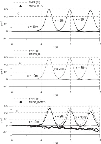
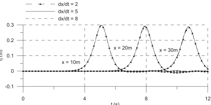
c , h is the water depth (taken as 1 m) over the flat bed of the tank spanning 40m from the wavemaker. A relatively long simulation has been carried out to examine whether there is any unacceptable diffusion due to the interpolation of the velocity for the inner nodes using the IMLPG_R method. The above equation for the motion of the wavemaker is implicit; hence Newton-Raphson iteration is used to solve it as suggested by Goring [46]. The wave time histories at 10m, 20m and 30m away from the wavemaker are shown and compared with the results from fully nonlinear potential theory (FNPT) [51] in Fig. 1. From Figs. 1a and 1b, one can see that the results from the IMLPG_R and MLPG_R-PG are almost same as those from the FNPT model, which may demonstrate that the diffusion caused by the interpolation in the IMLPG_R method is negligible. The slight decrease in the wave height at 20m (0.295m) and 30m (0.29m) for all three models are due to the amplitude dispersion of the nonlinear waves (Yan [50], Sriram [52]). On the other hand, the wave heights and wave profiles from the MLPG_R-MPG (Fig. 1c) are considerably different from others, clearly showing the spurious energy loss of this method. Further, there is a visible, though small, oscillation on the free surface obtained by using the MLPG_R-MPG even before the wave reaches the locations where the time histories are recorded. These oscillations are caused due to the non-conservation of the momentum for the particles as indicated before.

with the MLPG_R-PG that does not require the interpolation. The total number of nodes used for this simulation is 16,856. These simulations are run on DELL Latitude E4200 with 3GB RAM and 1.2GHz processors.

In order to investigate the relative errors in the numerical scheme discussed in Section 2.3, an error analysis has been performed in the way similar to [30]. The relative error is defined as,

r r c r E

K K K

where

³

r A

r r dA

2

K

K with Ar being the area over which the error is estimated; Kc is the

computed results from the numerical method; K_r is the reference solution. The reference solution in the present case is taken from the FNPT model [51]. The relative errors for these methods obtained by integration over the whole tanks at each of time steps are shown in Fig. 2. It can be observed that the errors of the MLPG_R-MPG are generally larger than those for other two methods, whereas the MLPG_R-PG and IMLPG_R are in the same order of accuracy in this case.

0 4 8 12 t (s)

-0.1 0 0.1 0.2 0.3

K

(m

)

FNPT [51] MLPG_R-PG

x = 10m

x = 20m

x = 30m

a)

0 4 8 12

t (s) -0.1

0 0.1 0.2 0.3

K

(m

)

FNPT [51] IMLPG_R

x = 10m

x = 20m

x = 30m

b)

0 4 8 12

t (s) -0.1

0 0.1 0.2 0.3

K

(m

)

FNPT [51] MLPG_R-MPG

x = 10m

x = 20m

_{x = 30m}

c)

0 4 8 12 t (s)

-8 -4 0 4

Log

(

E

r)

IMLPG_R MLPG_R-PG MLPG_R-MPG

Fig.2. Relative Error for the three numerical schemes for solitary wave propagation.

0 4 8 12

t (s) -0.1

0 0.1 0.2 0.3

K

(m

)

dx/dt = 2 dx/dt = 5 dx/dt = 8

x = 10m

x = 20m _{x = 30m}

0 4 8 12 t (s)

-0.1 0 0.1 0.2 0.3

K

(m

)

dx = 0.03 dx = 0.04 dx = 0.05

x = 10m

x = 20m x = 30m

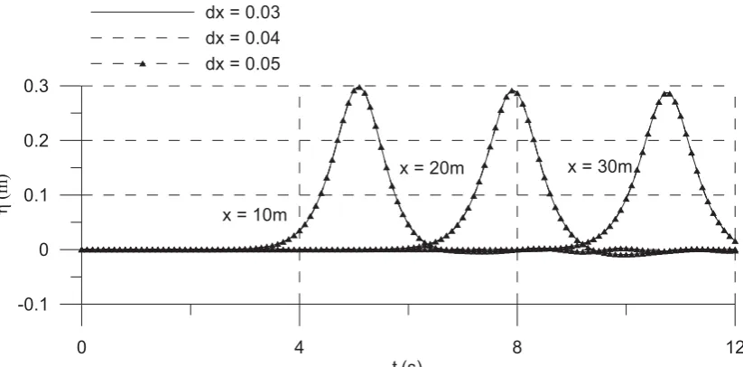
Fig.4. Comparison of free surface profile for different spacings of nodes using constant time step of 0.01s, recorded at x= 10m, 20m and 30m, respectively.

5.2 Breaking wave over a slope beach

In this section, the simulation of overturning wave is presented to show the nodal

distributions obtained using the three methods and to compare results with

experimental data. The case considered for this purpose is the propagation of solitary waves over a beach with a slope of 1:15. The solitary wave is generated by a piston-type

wavemaker according to the theory given by Goring [46] as described abovebut the wave

height is taken as 0.45m above the rest water level with the water depth being 1m over

the flat bed spanning 10m from the wavemaker to the toe of the slope beach. The

example is similar to that used in Sriram and Ma [38]. In the simulation, the initial

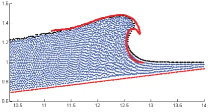
distances between the particles are selected as 0.025m and the time step is taken as 0.0032s, giving dx/dt=7.8 m/s. Sriram and Ma [38] and Ma and Zhou [26] have shown that these parameters are appropriate to give convergent results. The snapshots of the free surface profiles and the configuration of water particles at t=3.30s obtained by using three algorithms are shown in Fig. 5, 6 and 7 respectively, together with the experimental data

from Li and Raichlen [47]. It can be seen from the figure that in the MLPG_R-PG

simulations particles at some places are severely scattered (shown by the black circles in the figure). In contrast, the particles are distributed more regularly and uniformly when one uses the MLPG_R-MPG. The distribution of particles in the IMLPG_R simulations is better than that of the MLPG_R-PG but not as good as that in the MLPG_R-MPG. However, on the other hand, the free-surface profile from the MLPG_R-PG and IMLPG_R are nearer to the experimental results compared with those from the MLPG_R-MPG simulation perhaps due to the energy loss caused by the method. The corresponding pressure time histories recorded at points x = 10.5m and 12.5m are depicted in Fig. 8 for all the three algorithms. It can be observed that there are big spikes

in the result obtained by using the MLPG_R-PG while they are not so evident in the

particles in the neighboring region (gaps). In summary, the IMLPG_R results for this case are better than those from the MLPG_R-MPG and the MLPG_R-PG algorithms in terms of both surface elevations and pressure time histories.

Fig.5. Comparison of the free surface profile from the MLPG_R-PG (black dots)

at the overturning position with experimental results (red line). The areas circled show that the particles are significantly scattered.

Fig.6. Comparison of the free surface profile from the MLPG_R MPG (black dots) at the overturning position with experimental results (red line)

0 2 4 6 8 t (s)

0 0.2 0.4 0.6 0.8

P/

U

gh

IMLPG_R MLPG_R-PG MLPG_R-MPS

x= 10.5

x=12.5

Fig.8. Comparisons of the pressure time history at two points on the slope bottom.

5.3. Interaction between a fixed rigid plate and a wave generated by an initial elevation

The interaction between a small wave and a fixed rigid plate is reported in this section. The surface wave is generated by an impulse-type elevation on the free surface profile at initial time given by

° ¯ ° ® ­

t

d » ¼ » «

¬

«

1 0

1 0 0

1 0

) ( cos 1 2 ) (

d x x

d x x x

x d a

x

S K

(23)

wherex0 =0.7m is the peak position of the initial profile relative to the elastic plate, a=

0.05m is its amplitude and d1 = 0.5m is the points at which the elevation becomes zero.

Fig.9. Illustration of Computational domain.

0 1 2 3 4

t (s) -0.02

0 0.02 0.04 0.06

K

(m

)

FNPT [51] IMLPG_R MLPG_R-PG MLPG_R-MPG

Fig.10. Comparison of the free surface time histories at x=0.7m from three schemes.

0 1 2 3 4

t (s) -16

-12 -8 -4 0

Log

(

E

r)

IMLPG_R MLPG_R-PG MLPG_R-MPG

Fig.11. Relative Error for the three schemes with respect to FNPT solution.

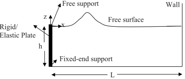
z x

L

Wall

Free surface Rigid/

Elastic Plate

Fixed-end support Free support

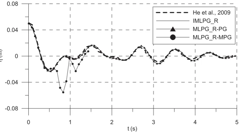
5.4. Interaction between an elastic plate and a wave generated by an initial elevation The configuration of this case is very similar to that in Section 5.3 but the left end of the tank is replaced by an elastic plate that is free at its top end and fixed to the tank bed, as has been seen in Fig. 9. The elastic parameters of the plate is EI/gh4=0.01 and the

product of its density (s) and thickness (s) is assumed to be s s/ h = 0.1. The

deflection of the plate in horizontal direction is denoted by (z,t), where z is the

coordinate in the vertical direction measure from the bed. The surface wave is generated in the same way as in Section 5.3. The setup of this example is the same as one presented

by He et al [13], whose results will be used to validate results of the present method.

To simulate this case, the particles in fluid domain are distributed with initial distance of dx=0.05m; the elements of the plate have a similar size and the time step is

chosen as dt=0.0088s, which gives dx/dt=5.68 m/s. The deflection at the centre of the

plate and the free surface time history at x=0.7m for the three methods are compared with

the numerical results of He et al [13] in Fig. 12 and 13. The figure shows that the simulation using the MLPG_R-MPG breaks down as reported in Section 5.3, and also that a reasonably good agreement between the results from the MLPG_R-PG and IMLPG_R with that of numerical results in [13], in particular up to the time t =2s is achieved. After this time, difference between results of the MLPG_R-PG /IMLPG_R and those of He et al [13] is visible, though is still acceptable. One of reasons for the difference would be because the model we use here is different from that used in [13]. They adopted the Eigen function expansion for the structure equation and the potential theory for the water waves while we solved the structures equations by numerically integrating Eq. (22) and the Navier–Stokes equations for water waves.

0 1 2 3 4 5

t (s) -0.6

-0.4 -0.2 0 0.2 0.4

[

m

He et al., 2009 IMLPG_R MLPG_R-PG MLPG_R-MPG

0 1 2 3 4 5

t (s) -0.08

-0.04 0 0.04 0.08

K

m

He et al., 2009 IMLPG_R MLPG_R-PG MLPG_R-MPG

Fig.13. Comparison of the free surface time history at x=0.7m (the elastic plate is free on its top with

EI/gh4=0.01; s s/ h = 0.1).

The other reason for visible difference may be due to the number of particles is not sufficient large and/or the time step is not sufficient small. In order to look at the effects

of the number of particles and time step in this case, we have further investigated the

convergent properties in this case for the IMLPG_R method. The comparison of the deflection at the centre of the plate for the above case obtained by using different values of dx/dt with dx=0.05m is shown in Fig.14. The figure shows that the numerical results

are almost the same and that dx/dt = 5.68 used in the above case are appropriate. The

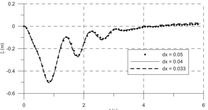
similar investigation is also carried out by varying the initial distance between fluid particles, keeping the element size for the plate similar to the particle distance. The results for dx=0.05, 0.04 and 0,033 are depicted in Fig. 15 and agree well with each other, demonstrating the dx=0.05 employed in Figs. 12-13 are appropriate as well.

0 2 4 6 t (s)

-0.6 -0.4 -0.2 0 0.2

[

m

dx/dt = 6.68 dx/dt = 5.68 dx/dt = 5

Fig.14. Comparison of the plate central deflections for different time steps having constant grid spacing (dx=0.05m, elastic plate is free on its top with EI/gh4=0.01; s s/ h = 0.1).

0 2 4 6

t (s) -0.6

-0.4 -0.2 0 0.2

[

m

dx = 0.05 dx = 0.04 dx = 0.033

0 1 2 3 4 5 t (s)

0 10 20 30 40

No

. o

f

it

e

rat

io

ns

Aitkens Relaxation Constant relaxation = 0.8

Fig. 16 Comparisons of the number of iteration corresponding to different relaxation parameters (elastic plate is free on its top with EI/gh4=0.01; s s/ h = 0.1).

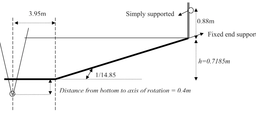
Fig.17a. Illustration of experimental setup similar to that used in [48].

3.95m

h=0.7185m

Distance from bottom to axis of rotation = 0.4m 1/14.85

Simply supported

Fig. 17b Details of the plate configurations in experiments [48] (not to the scale).

5.4. Violent Breaking wave interaction with an elastic plate

As reported earlier in the literature, numerical modelling of violent breaking wave interaction with elastic structures is limited. There are some numerical studies for the dam breaking interaction with elastic solids [23, 24, 25] and experimental studies for dam breaking interaction with the elastic gate [20]. In this section, our numerical model will be applied to simulate violent wave interactions with an elastic plate, which is similar to that in experimental studies of [48]. This can further validate the present method. The experiments [48] are carried out in a wave flume with a flap wave maker installed on the left side to generate waves as shown in Fig. 17a. An elastic plate with a height of 1 m and a width of 0.65m is mounted at the right end, fixed at the bottom and simply supported at 0.88m from the bottom, as shown in Fig. 17b. The length of the flume between the wave maker and plate is 14.5m with a bottom slope of 1:14.85 starting at 3.95m from the wave maker. The density and Youngs modulus of the plate are

1190Kg/m3 and 3250MPa, respectively.

During the experiments reported in [48], a solitary wave was generated using the theory given by Guizien and Barthelemy [54], which specified the angle of the paddle as a function of time. Further details can be found in [49, 50]. In our numerical simulation,

the case with the water depth (h) of 0.7185m, the wave amplitude (H) of 0.08m on the

flat bottom part and plate thickness of 4mm is considered and discussed in this section.

This corresponds to a ratio of the amplitude to the water depth (H/h) of 0.11. Based on

the tests in the previous section and our tests on this specific case, 86,670 particles are employed in the fluid domain, giving the initial distance between water particles is about dx=0.0089 m. The element size for discretising the plate is similar to dx; and the time step (dt) is chosen as 0.0018s (corresponding to dx/dt = 4.95m/s). The experiment [48]

h = 0.7185m at rest

30mm

880mm 1000m

Thickness 4mm

Simply Support

Fixed - End Support 2 Cylinder 20mm

backlash 40mm

has shown that an overturning wave is formed and impacts on the plate, leading to violent wave interaction with the plate.

Fig. 18. Experimental plate deflection at 0.3623m from the bottom of the plate and the corresponding spatial wave profile images taken in the experiment[48]. Circled one showing a small leakage of water

through the side gap of the plate.

The experimental and numerical deflections of the plate at 0.3623m from the bottom are shown in Fig.18 and Fig. 19a along with several spatial wave profiles at some time instants. The two figures are largely similar, though there is inevitable discrepancy. Specifically, both curves have two peaks, with the largest one being about 2.5cm and occurring at about 0.43s in the experimental results, compared to 2.4cm and 0.42s respectively in the numerical result. In addition, the wave profiles near the structure

shown at some corresponding time instants are also very similar. Further, it is noted that

there is a negative deflection before the wave impacts on the plate observed in the experiment. This is unclear to us, as the plate should not be influenced before it is impacted, as the supports are fixed at the bottom upto 30 mm and simply supported at the top (Fig. 17b).

The modal frequency of the plate is evaluated using hammer impact test by

Kimmoun et al. [48] and is about 4.37Hz. Our numerical deflections of the plate after the

wave impact obtained by the three methods discussed are shown in Fig. 19b, which indicated that the frequency of the plate vibration after impact is about 4.9Hz in the

results of IMLPG_R, close to the one obtained using hammer test. Further, the

MLPG_R-MPG result suffers numerical damping with its peak deflection being considerably less than the experimental one. Specifically, the peak deflection is reduced by 12.5%. In contrast, the simulation using the MLPG_R-PG method breaks down in this case.

problem not only with our simulation but also with BEM modeling as reported in [49].

Another reason related only to the discrepancy in the natural frequency is perhaps due to the added mass and restoring force of the plate in the hammer impact test (carried out in the absence of water) being likely different from that when wave impacts on the plate.

Fig. 19a. Deflection of the plate at 0.3623 m from the bottom of the plate obatined using numerical simulation (IMLPG_R), and the corresponding spatial wave profiles.

The pressure time history on the plate at a point 0.045m from the bottom is shown in Fig. 20. The figure also shows the corresponding results for a rigid plate with the same size and configuration. It can be observed that in the case for elastic plate, the pressure

reaches a maximum value of about 16KN/m2 at 0.01s. After that it fluctuates at around

2KN/m2. Whereas, the impact pressure for the rigid wall is about 18KN/m2 at 0.01s.

After that it has a mean value of about 2KN/m2 before the second impact occurs. Thus,

the ratio of maximum pressure of rigid plate to that of elastic plate is about 1.125. It is noted that pressure time histories due to violent breaking simulated by other meshless methods (such as discussed by Khayyer and Gotoh [52]) often contain spurious high frequency fluctuations but this figure shows that the pressure time history produced by the present meshless method is quite smooth. It is also noted that it would be desired to compare numerical pressure results with experiment data. Unfortunately the experimental pressure was not measured for this test case, owing to the experimental difficulties as reported in [48]. However, the pressure from the MLPG_R method has been compared with the experimental data in the case for waves impacting on rigid

The comparison of the pressure time histories from three methods is depicted in Fig. 21a. The figure shows that the IMLPG_R pressure impact is higher than those from other two methods. Further, there are two distinct peaks within a short time is noticed in the simulation using the MLPG_R-MPG. This small pressure from the MLPG_R-MPG is likely related to the spurious damping as indicated above. In addition, the simulation using MLPG_R-PG gives some negative pressures at 0.21s, which is unreasonable. This is due perhaps to spuriously scattered particle distribution as shown in Fig. 21b, which eventually leads the breaking down of the MLPG_R-PG simulation.

-0.2 0 0.2 0.4 0.6 0.8 1 1.2 1.4

t (s) -1

-0.5 0 0.5 1 1.5 2 2.5 3

[

cm

Kimmoun et al., [48] IMLPG_R MLPG_R-MPG

MLPG_R-PG

Fig.19b. Comparison of the structure deflection at 0.3623 m of the plate obtained by different methods. The excitation of the first natural frequency of the plate is also depicted. The first mode frequency of 4.37 Hz is

obtained by hammer test [48]

6. Conclusion

This is a first paper to extend the MLPG_R (Meshless local Petrov Galerkin method based on Rankine source solution) method to numerically simulate interaction between violent breaking waves and elastic structures. One novel point of this paper is that the water wave is simulated using a robust improved MLPG_R (IMPG_R) algorithm that uses newly developed technique to update the velocity and position of fluid particles. In this technique, the pressure gradient used for updating particle velocities is evaluated directly by the simplified finite difference scheme (SFDI) while the pressure gradient used for updating particle position is estimated by the modified SFDI in which the pressure at the point concerned is replaced by a minimum pressure. This technique can well conserve momentum of fluid whereas keeping the fluid particle motion relative

f= 4.9 Hz (1st Mode = 4.37Hz in

stable. The numerical testes show that it works well. The second novel point of this paper is that a Near-Strongly Coupled and Partitioned (NSCP) procedure is proposed. In this procedure, the equations for fluid and structure are solved iteratively and so solution at the end of each step can satisfy the equations and conditions on the interface between fluid and structure to the level specified. During the iteration in each time step, the matrix for fluid equation is kept unchanged, enhancing the computational efficiency. In order to reduce the number of iteration in each time step, varying relaxation parameter is introduced into the NSCP procedure, which is very effective based on our numerical tests.

The method and techniques are validated by using experimental and other numerical data. This includes the comparison between our results and those in literature for the

several cases, such as (1) overturning waves over a slope; (2) interaction between an

elastic plate and a wave generated by specifying initial elevation; and (3) interaction between an elastic plate and violent breaking waves. In all cases considered, reasonably good agreement is achieved.

Some results are presented to show the convergent property of the method. They demonstrate that convergent numerical results can be achieved if the initial distance of particles (dx) and the length of time steps (dt) are appropriately chosen. The range of the ratio of dx/dt may be selected as 4-7 m/s for the waves considered in this paper, similar to what we have found for wave only problems.

Limited numerical tests show that the proposed meshless method in this paper can produce relatively smooth pressure time history due to violent breaking waves, which is important for successfully modeling wave-structure problems. The method has been applied to 2D problems but will be extended to dealing with 3D cases in our future work.

0 0.1 0.2 0.3

t (s) 0

4000 8000 12000 16000

P (N

/m

m

2)

Elastic wall Rigid Wall

0 0.2 0.4 t (s)

-4000 0 4000 8000 12000 16000

P (

N

/mm

2)

IMLPG_R MLPG_R-MPG MLPG_R-PG

Fig. 21a. Pressure time history at 0.045m from the bottom of the plate.

`

Fig.21b. Example of node distribution at an instant using MLPG_R-PG.

7. Acknowledgement

The authors would like to acknowledge Newton International Fellowship funded by the Royal Society, the Royal Academy of Engineers and British Academia for the grants. We would also like to thank Dr. Oliver Kimmoun, Ecole Centrale de Marseille, France for sharing their experimental measurements with us. Further, we would like to thank the reviewer for his constructive comments.

8. Reference

[1] X.J. Chen, Y. Wub, W. Cuib, J. Jensen, Review of hydroelasticity theories for

global response of marine structures, Ocean Engg, 33 (2006) 439–457.

[2] O.M.Faltinsen, M. Landrini M.Greco, Slamming in marine applications, J. Engg. Mathem., 48 (2004) 187-217.

[3] K. Tanizawa, A nonlinear simulation method of hydro-elastic problem, Proc. of

Symp. on Nonlinear and Free-Surface Flow, 5 (1997) 37-40.

[4] K. Tanizawa A Time-domain Simulation method for hydroelastic impact problem.

Proc. of Hydroelasticity'98 Hydroelasticity in marine technology (1998).

[5] M. Greco, A Two-dimensional Study of Green-Water Loading. Ph. D. thesis, Dept.

Marine Hydrodynamics, NTNU, Trondheim, Norway, 2001.

[6] J.H Kyoung, S.Y. Hong and B.W. Kim, FEM for time domain analysis of

hydroelastic response of VLFS with fully nonlinear free surface condition, Int. J. Offshore and Polar Engineering, 16 (3) (2006)168-174.

[7] J.H Kyoung, and S.Y. Hong, Time domain analysis of hydroelastic response of

VLFS considering horizontal motion. Int J Offshore Polar Eng, 18 (1) (2008) 21– 26.

[8] X. Liu, S. Sakai, Time Domain Analysis on the dynamic response of a flexible

floating structure to waves, Journal of Engineering Mechanics, 128(1) (2002) 48-56.

[9] N.M. Sudharsan , K. Murali, K. Kumar, Preliminary Investigations on Non-linear

Fluid Structure Interaction of an Offshore Structure, Journal of Mechanical Engineering Science, Proceedings of the Institution of Mechanical Engineers U.K. Part C, 217(2003) 759 - 765.

[10] G.X. Wu, R. Eatock Taylor, Finite element analysis of two-dimensional non-linear transient water waves. Applied Ocean Research, 16 (1994) 363-372.

[11] T. Tsubogo The Motion of an Elastic Disk Floating on Shallow Water in Waves. Proceedings of the Eleventh International Offshore and Polar Engineering Conference, Stavanger, Norway, June 17-22 (2001) 229-233

[12] R.C. Ertekin, J.W. Kim, Hydroelastic Response of a Floating, Mat-Type Structure in Oblique, Shallow-Water Waves, J. Ship Research, 43 (4) (1999) 241-254.

[13] G. He, M. Khasiwagi, and C. Hu, Nonlinear Solution for Vibration of Vertical Elastic Plate by Initial Elevation of Free Surface, In Proceedings of the Nineteenth (2009) International Offshore and Polar Engineering Conference, Osaka, Japan, June 21-26, 3 (2009) 406-413.

[14] Z.Z. Hu, D.M. Causon, C.G. Mingham, L. Qian, Numerical simulation of floating bodies in extreme free surface waves, Nat. Hazards Earth Syst. Sci., 11 (2011) 519– 527.

[15] L Qian, DM Causon, CG Mingham, DM Ingram A Free-Surface Capturing Method for Two Fluid Flows with Moving Bodies, Proceedings of the Royal Society of

London: A 462 (2006),21-42.

[16] B. Rogers, R. Dalrymple, P. Stansby, Simulation of caisson breakwater movement using 2-D SPH, Journal of Hydraulic Research, 47 (2009)135–141.

[17] P. Omidvar, P. Stansby, B. Rogers, Wave body interaction in 2D using smoothed particle hydrodynamics (SPH) with variable particle mass, Int. J. Numer. Meth. Fluids, online DOI: 10.1002/fld.2528.

[19] N. Kuroda, S. Ushijima, Numerical prediction of interactions between wave flows and flexible structures with 3D MICS, Proceedings of the Eighteenth International offshore and polar Engineering Conference, Vancover, Canada, July 6-11 (2008) 108-115.

[20] C. Antoci, M. Gallati, S. Sibilla , Numerical simulation of fluid–structure interaction by SPH, Comput. Struct., 85(2007) 879–890.

[21] G. Oger, L. Brosset, P.M. Guilcher, E. Jacquin, J.B. Deuff, D Le

Touzé, Simulations of Hydro-elastic Impacts Using a Parallel SPH

Model, Proceedings of the Nineteenth (2009) International Offshore and Polar Engineering Conference, Osaka, Japan, (2009) 316-324.

[22] R. Issa, D. Violeau, E.S. Lee, H. Flament, Modelling Nonlinear Water Waves with RANS and LES SPH models, Chapter 14 in Advances in Numerical Simulation of Nonlinear Water Waves (ISBN: 978-981-283-649-6, edited by Q.W. Ma) (Vol. 11 in Series in Advances in Coastal and Ocean Engineering). World Scientific Publishing Co. Pte. Ltd., 75- 128 (2010).

[23] A. Rafiee, K. Thiagarajan, An SPH projection method for simulating fluid-hypoelastic structure interaction, Comput. Methods Appl. Mech. Engrg. 198 (2009) 2785–2795.

[24] CJK. Lee , H. Noguchi , S. Koshizuka , Fluid–shell structure interaction analysis by coupled particle and finite element method. Computers and Structures, 85(2007) 688–697.

[25] J. Marti, S. Idelsohna, A Limache, N Calvo, J D’Elía, A fully coupled particle method for quasi-incompressible fluid-hypoelastic structure interactions, Mecánica Computacional Vol XXV, 809-827. A Cardona, N Nigro, V Sonzogni and M Storti. (Eds.) 2006.

[26] Q.W. Ma, J.T. Zhou, MLPG_R Method for Numerical Simulation of 2D Breaking Waves, CMES, 43, 3 (2009) 277-303.

[27] J.T, Zhou, Q.W. Ma, MLPG Method based on Rankine source solution for

modelling 3D Breaking Waves, Computer Modeling in Engineering & Sciences (CMES), 56(2) (2010)179-210.

[28] J.T. Zhou, Q.W. Ma. L. Zhang, Numerical investigation on violent wave impacts on offshore wind energy structures with meshless method., Proceedings of the Nineteenth (2009) International Offshore and Polar Engineering Conference, Osaka, Japan (2009) 503-509.

[29] S. Koshizuka, Y. Oka, Moving-particle semi-implicit method for fragmentation of incompressible fluid. Nuclear Science and Engineering, 123 (1996) 421– 434. [30] Q.W. Ma Meshless Local Petrov- Galerkin Method for Two-dimensional Nonlinear

Water Wave Problems. Journal of Computational Physics, 205 (2) (2005) 611-625. [31] J.T. Zhou, Q.W. Ma and S. Yan Numerical Implementation of Solid Boundary

Conditions in Meshless Methods. In Proceedings of the Eighteenth (2008) International Offshore and Polar Engineering Conference Vancouver, BC, Canada, July 6-11, 2008.

[32] Q.W. Ma, A New Meshless Interpolation Scheme for MLPG_R Method. Computer Modeling in Engineering & Sciences, 23 (2) (2008) 75-89.

[34] J. Bonet, T.S. Lok, Variational and momentum preservation aspects of smooth particle hydrodynamic formulation. Computer Methods in Applied Mechanics and Engineering 180 (1999) 97–115.

[35] G.L. Vaughan, T.R. Healy, K.R. Bryan, A.D. Sneyd, R.M. Gorman, Completeness, conservation and error in SPH for fluids. International Journal for Numerical Methods in Fluids 56 (2008) 37–62.

[36] A. Khayyer , H. Gotoh A higher order Laplacian model for enhancement and stabilization of pressure calculation by the MPS method., Applied Ocean Research, 32 (1) (2010) 124-131.

[37] Y. Suzuki, S. Koshizuka, Y. Oka, Hamiltonian moving-particle semi-implicit (HMPS) method for incompressible fluid flows. Computer Methods in Applied Mechanics and Engineering 196 (29-30) (2007) 2876–2894.

[38] V. Sriram, Q.W. Ma, Simulation of 2D breaking waves by using improved

MLPG_R method, Proceedings of 20th International Offshore and Polar

Engineering Conference, Beijing, China, 3 (2010) 604-610

[39] T.J.R. Hughes, The finite element method – linear static and dynamic finite element analysis, Prentice-Hall, Inc. New Jersey, 1987

[40] G.P. Guruswamy, Time-accurate unsteady aerodynamic and aeroelastic calculations of wings using Euler equations, AIAA Paper No. 88-2281, AIAA 29th Structures, Structural Dynamics and Materials Conference, Williamsburg, Virginia, 18-20 April 1988.

[41] C. Farhat, M. Lesoinne, P. LeTallec, Load and motion transfer algorithms for fluid/structure interaction problems with nonmatching discrete interfaces: Momentum and energy conservation, optimal discretization and application to aeroelasticity,Comput. Methods Appl. Mech. Engrg. 157 (1998) 95-114.

[42] C. Farhat, M. Lesoinne, Two Efficient Staggered Procedures for the Serial and Parallel Solution of Three-Dimensional Nonlinear Transient Aeroelastic Problems, Computer Methods in Applied Mechanics and Engineering, 182 (2000) 499-516.

[43] S. Piperno, C. Farhat, B. Larrouturou, Partitioned procedures for the transient solution of coupled aeroelastic problems, Comput. Methods Appl. Mech. Engrg. 124 (1995) 79-711.

[44] A.W. Wall, S. Genkinger, E. Ramm, A strong coupling partitioned approach for fluid-structure interaction with free surfaces, Computers and fluids, 36(2007) 169-183.

[45] B. Irons, RC. Tuck, A version of the Aitken accelerator for computer implementation. Int J Numer Methods Engrg;1 (1969) 275–7.

[46] D.G. Goring, Tsunamis – the propagation of long waves on to a shelf, Ph.d. thesis, California Institute of Technology, Pasadena, 1979.

[47] Y. Li, F. Raichlen, Discussion- Breaking Criterion and Characteristics for Solitary

Waves on Slope, J. Waterw., Port. Coastal, Ocean Eng., 124 (1998) 329-335. [48] O. Kimmoun , S. Malenica , Y.M. Scolan, Fluid structure interactions occuring at a

flexible vertical wall impacted by a breaking wave. In Proceedings of the Nineteenth (2009) International Offshore and Polar Engineering Conference,