TENET: Tail-Event driven NETwork risk

City, University of London Institutional Repository

Citation:

This is the accepted version of the paper.

This version of the publication may differ from the final published

version.

Permanent repository link:

Link to published version:

Copyright and reuse: City Research Online aims to make research

outputs of City, University of London available to a wider audience.

Copyright and Moral Rights remain with the author(s) and/or copyright

holders. URLs from City Research Online may be freely distributed and

linked to.

TENET: Tail-Event driven NETwork risk

∗

Wolfgang Karl H¨

ardle

Weining Wang

Lining Yu

February 8, 2016

Abstract

CoVaR is a measure for systemic risk of the networked financial system con-ditional on institutions being under distress. The analysis of systemic risk is the focus of recent econometric analyzes and uses tail event and network based

tech-niques. Here, in this paper we bring tail event and network dynamics together into one context. In order to pursue such joint efforts, we propose a semiparametric

measure to estimate systemic interconnectedness across financial institutions based on tail-driven spillover effects in a high dimensional framework. The systemically important institutions are identified conditional to their interconnectedness

struc-ture. Methodologically, a variable selection technique in a time series setting is applied in the context of a single-index model for a generalized quantile regression

framework. We could thus include more financial institutions into the analysis to measure their tail event interdependencies and, at the same time, be sensitive to non-linear relationships between them. Network analysis, its behaviour and

dy-namics, allows us to characterize the role of each financial industry group in 2007 - 2012: the depositories received and transmitted more risk among other groups,

the insurers were less affected by the financial crisis. The proposed TENET - Tail Event driven NETwork technique allows us to rank the Systemic Risk Receivers and Systemic Risk Emitters in the U.S. financial market.

∗_{Financial support from the Deutsche Forschungsgemeinschaft (DFG) via SFB 649 “ ¨Okonomisches}

Risiko”, IRTG 1792 “High-Dimensional Non-Stationary Times Series” and Sim Kee Boon Institute for Financial Economics, Singapore Management University are gratefully acknowledged.

†_{Professor at Ladislaus von Bortkiewicz Chair of Statistics, C.A.S.E. - Center for Applied Statistics}

and Econometrics, Humboldt-Universit¨at zu Berlin, Unter den Linden 6, 10099 Berlin, Germany. Email: [email protected].

‡_{Professor at Ladislaus von Bortkiewicz Chair of Statistics, C.A.S.E. - Center for Applied Statistics}

and Econometrics, Humboldt-Universit¨at zu Berlin, Unter den Linden 6, 10099 Berlin, Germany. Email: [email protected].

§_{Research associate at Ladislaus von Bortkiewicz Chair of Statistics, C.A.S.E. - Center for Applied}

Keywords: Systemic Risk, Systemic Risk Network, Generalized Quantile, Quantile Single-Index Regression, Value at Risk, CoVaR, Lasso

JEL: G01,G18,G32,G38, C21, C51, C63.

1

.

Introduction

Systemic risk endangers the stability of the financial market, the failure of one institution may harm the whole financial system. The sources of risk are complex, as both exogenous and endogenous factors are involved. This calls for a study on a financial network which accounts for interaction between the agents in the financial market. Although the notion

systemic risk is not novel in academic literature (see, e.g, Minsky (1977)), it had been neglected both in academia and in the financial risk industry until the outbreak of the financial crisis in 2008. Some financial institutions collapsed, even some major ones like Lehman Brothers, Federal Home Loan Mortgage Corporation (Freddie Mac), and Federal National Mortgage Association (Fannie Mae). The magnitude of repercussions caused by this financial crisis and its complexity revealed a significant flaw in financial regulations. As in the past, regulations had been focused primarily on stability of a single financial institution. The detailed actions involved the establishment of Financial Stability Board (FSB) after G-20 London summit in 2009, integration of systemic risk agenda into Basel III in 2010 prior to the G-20 meeting in Seoul, and enacting the Dodd Frank Wall Street Reform and Consumer Protection Act (‘Dodd Frank Act’) in the U.S. in 2010, which is said to have bought the most radical changes into the U.S. financial system since the Great Depression.

In this context, the focus is onsystemically important financial institutions (SIFIs) whose failure may not only impair the functioning of the financial system but also have adverse effects on the real sectors of the economy. Therefore, we face several challenges such as identifying SIFIs, studying the propagation mechanism of a shock in a system, or in a network formed by financial institutions, investigating the response of a system to a shock as a whole network and establishing a theoretical framework for systemic risk.

Although systemic risk is a relatively straightforward concept aimed at measuring risk

structural frameworks, and quantitative modelling with the emphasis on empirical anal-ysis. The quantitative literature can be further classified by statistical methodology into quantile regression based modelling such as linear bivariate model by Adrian and Brun-nermeier (2011), Acharya et al. (2012), Brownlees and Engle (2015), high-dimensional linear model by Hautsch et al. (2015), partial quantile regression by Giglio et al. (2012) and by Chao et al. (2015). Further approaches include principal-component-based

analy-sis, e.g. by Bisias et al. (2012), Rodriguez-Moreno and Pe˜na (2013) and others; statistical modelling based on default probabilities by Lehar (2005), Huang et al. (2009), and others; graph theory and network topology, e.g. Boss et al. (2006), Chan-Lau et al. (2009), and Diebold and Yilmaz (2014).

Our paper belongs to the quantitative group of the aforementioned literature, namely, modelling the tail event driven network risk based on quantile regressions augmented with non-linearity and variable selection in a high dimensional time series setting. Our method is in nature different from Acharya et al. (2012) and Brownlees and Engle (2015)’s method. Acharya et al. (2012) has measured the systemic risk relevance without captur-ing the network effects of liquidity exposure, and Brownlees and Engle (2015) analyze the risk of a specific asset given the distress of the whole system, which is a reverse of our system at institutional analysis, and their method would capture little spillover effects. Therefore, we believe, that our method is a good addition to the literature of systemic risk measures. Also compared to Diebold and Yilmaz (2014), we focus more on the tail event driven interconnectedness, which cannot be captured by conditional correlation. As a starting point of our research we take co-Value-at-Risk, or CoVaR, model by Adri-an Adri-and Brunnermeier (2011) (from here on abbreviation as AB), where ‘co-’ stAdri-ands for ‘conditional’, ‘contagion’, ‘comovement’. To capture the tail interconnectedness between the financial institutions in the system AB evaluate bivariate linear quantile regressions for publicly traded financial companies in the U.S..

The assumption of non-linear relationship between returns of financial companies is moti-vated by previous work by Chao et al. (2015), who find that the dependency between any pair of financial assets is often non-linear, especially in periods of economic downturn. Moreover, non-linearity assumption is more flexible especially in a high dimensional set-ting where the system becomes too complex to support the belief of linear relationships. From the 2012 U.S. financial company list from NASDAQ, we select 100 financial

institu-tions consisting of the top 25 financial instituinstitu-tions from each industry group: Depositories, Insurance companies, Broker-Dealers and Others. These four groups are divided by S-tandard Industrial Classification (SIC) codes. Our model is evaluated, based on weekly log returns of these 100 publicly traded U.S. financial institutions. Firm specific charac-teristics from balance sheet information such as leverage, maturity mismatch, market to book and size are added into the model as well. Furthermore, the macro state variables are also involved. The time period from 5 January, 2007 to 4 January, 2013 covers one recession (from December 2007 to June 2009) and several documented financial crises (2008 and 2011). Dividing companies by industry groups and including several market perturbations allows not only to select the key players for each time period, but also additionally to highlight the connections between financial industries, which can in turn provide additional information on the nature of market dislocations. In application we find out that there are more interconnectedness between 2008 and 2010. While the bank sector plays a major role in the financial crisis, the insurance companies, however, play more passive roles in term of risk transmission and risk reception. The most connected financial institutions with respect to incoming and outgoing links are ranked based on our network analysis. The new insight of our finding is that the non-linear relationships between financial firms are stronger during the financial crisis than the stable periods. In addition, to identify the systemically important firm, we weight the connections by firms’s market capitalization. The empirical findings suggest that our method can effec-tively identify the systemic risk relevant firms similar to the literature. Moreover, we can discover the asymmetry and non linearity of the firms’ dependency structure, which leads to more accurate measures in terms of backtesting performance. All the R programs for this paper can be found on www.quantlet.de or www.quantlet.de/d3/ia/.

2

.

Systemic Risk Modelling

In this section, we lay down the background and the basic setup of our systemic risk analysis, which can be divided into three steps.

2.1

.

Basic concepts

Traditional measures assessing riskiness of a financial institution such as Value at Risk (VaR), or expected shortfall (ES) are based either on company characteristics or inte-grated macro state variables which account for the general state of the economy. Thus, for example, the VaR of a financial institution i atτ ∈(0,1) is defined as:

P(Xi,t ≤V aRi,t,τ)

def

= τ, (1)

where τ is the quantile level, Xi,t represents the log return of financial institution i at

time t. AB propose, the risk measure CoVaR (Conditional Value at Risk) which takes spillover effects and the macro state of the economy into account. The CoVaR of a financial institution j given Xi at levelτ ∈(0,1) at time t is defined as:

PXj,t ≤CoV aRj|i,t,τ|Ri,t

def

= τ, (2)

where Ri,t denotes the information set which includes the event of Xi,t = V aRi,t,τ and Mt−1. Note that Mt−1 is a vector of macro state variables reflecting the general state of

the economy (see Section 4 for details of macro state variables).

We start with the concept of CoVaR, which is estimated in two steps of linear quantile regression:

Xi,t =αi+γiMt−1+εi,t, (3)

Xj,t =αj|i+γj|iMt−1+βj|iXi,t+εj|i,t, (4)

F−1

εi,t(τ|Mt−1) = 0 and Fεj−|1i,t(τ|Mt−1, Xi,t) = 0 are assumed. AB propose, in the first

step, to determine VaR of an institution i by applying quantile (tail event) regression of log return of company i on macro state variables. The βj|i in (4) has standard linear

regression interpretation, i.e. it determines the sensitivity of log return of an institution

d

VaRi,t,τ = ˆαi+ ˆγiMt−1, (5)

\

CoVaRAB_j|i,t,τ = ˆαj|i+ ˆγj|iMt−1+ ˆβj|iVaRd_i,t,τ, (6)

Thus, the risk of a financial institutionj is calculated via a macro state and a VaR of an institution i. Here the coefficientβb_j|i of (6) reflects the degree of interconnectedness. By

setting j to be the return of a system, e.g. value-weighted average return on a financial index, andito be the return of a financial company i, we obtain thecontribution CoVaR which characterizes how a companyiinfluences the rest of the financial system. By doing the reverse, i.e. by setting j equal to a financial institution and i to a financial system, one obtains exposure CoVaR, i.e. the extent to which a single institution is exposed to the overall risk of a system.

This approach allows us to identify the key elements of systemic risk, namely, network ef-fects, a single institution’s contribution to systemic risk and a single institution’s exposure to systemic risk. In our models, we expand AB’s method in three aspects. First of all, AB perform pairwise quantile regression, since two companies are not interacting in an isolated environment, all other interaction effects need to be considered. This motivates us to extend this bivariate model to a (ultra)high dimensional setting by including more variables into the analysis, hence a variable selection should be carried out. Secondly, a linear relationship between system return and a single institution’s return is assumed by AB. Hautsch et al. (2015) apply a linear LASSO based variable selection to select variables to estimate the VaR of the system. We enhance their methodologies by employ-ing the nonlinear models because of the complexity of the financial system. The flexible SIM will be implemented to allow the nonlinear relationship in this case. Thirdly, AB use average market valued asset returns weighted by lagged market valued total assets to calculate the system return, as they point out it may create mechanical correlation between a single financial institution and the value-weighted financial index. Instead of the regression on system return, we proposed two market capitalization weighted indices which combine the connectedness structure of the companies: the index of Systemic Risk Receiver and the index of Systemic Risk Emitter, to measure the systemic risk contribu-tions, and further to identify the systemically important financial institutions.

2.2

.

Step 1

V aR

Estimation

Xi,t = αi+γiMt−1+εi,t, (7)

d

VaRi,t,τ = αˆi+ ˆγiMt−1, (8)

Xi,t and Mt−1 are defined as in section 2.1. Note that the VaR is estimated by the linear

quantile regression (7) of log returns of an institution i on macro state variables. This is justified by the analysis of Chao et al. (2015), who found evidence of linear effects in regressing Xi,t onMt−1.

2.3

.

Step 2 Network Analysis

2.3.1. Connectedness Analysis

In this step, TENET builds up a risk interdependence network based on SIM for quantile regression with variable selection. Note that our model can be easily extended to the case of expectiles, which provide coherent risk measures. First the basic element of the network: CoVaR calculation has to be determined. As in equation (2), Xj represents

a single institution, and the CoVaR of institution j is estimated by conditioning on its information set. This information set will not only include the asset returns of other firms estimated and the macro variables used in the previous step, but also uses control variables on internal factors of institutionj, i.e. the company specific characteristics such as leverage, maturity mismatch, market-to-book and size. This setting will allow us to model the risk spillover channels among institutions mostly caused by liquidity or risk exposure. Our choice of information set is more comprehensive than AB, and a similar motivation can be found in Hautsch et al. (2015). Further, a systemic risk network is built motivated by Diebold and Yilmaz (2014). TENET captures nonlinear dependency as it is based on a SIM quantile variable selection technique. See Appendix for more details of the statistical methodology. More precisely:

Xj,t =g(βj>|RjRj,t) +εj,t, (9)

\

CoVaRT EN ET_j|Rj,t,τe

def

= _bg(βb>

j|Rje

e

Rj,t), (10)

b

D_j| e Rj

def

= ∂bg( b

β_j>_|RjRj,t)

∂Rj,t

|_Rj,t= e Rj,t =bg

0

(βb>

j|Rje

e

Rj,t)βb_j|

e

Rj. (11)

HereRj,t

def

= {X−j,t, Mt−1, Bj,t−1}is the information set which includespvariables,X−j,t

def

=

{X1,t, X2,t,· · · , Xk,t}are the explanatory variables including the log returns of all financial

insti-tutions. Bj,t−1are the firm characteristics calculated from their balance sheet information.

Define the parameters asβj|Rj

def

= {βj|−j,βj|M,βj|Bj}>. Note that there is no time symbol t in the parameters, since our model is set up based on one fixed window estimation, we can then apply moving window estimation to estimate all parameters in different win-dows. We define Rej,t

def

= {V aR[−j,t,τ,Mt−1,Bj,t−1}, VaRd−j,t,τ as the estimated VaRs from

(8) for financial institutions except forjin step 1, andβb_j|

e Rj

def

= {βb_j|−j,βb_j|M,βb_j|Bj}>. As in

equation (10) CoVaR comprises of not only the influences of financial institutions except for j, but also incorporates non-linearity reflected in the shape of a link function g(·).

Therefore, we name it CoVaR\ T EN ET which stands for Tail-Event driven NETwork risk with SIM model.1 Db_j|

e

Rj is the gradient measuring the marginal effect of covariates

eval-uated atRj,t =Rej,t, and the componentwise expression isDb_j|

e Rj

def

= {Dbj|−j,Dbj|M,Dbj|Bj}>.

In particular, Dbj|−j allows to measure spillover effects across the financial institutions

and to characterize their evolution as a system represented by a network. Note that in our network analysis we only include the partial derivatives of institution j with respect to the other financial institutions (i.e. Dbj|−j). The partial derivatives with respect to

institution’s characteristic variablesDbj|Bj and macro state variablesDbj|M are not

includ-ed. The reason is that we concentrate on spillover effects among firms in the network analysis.

The termnetwork refers to a (directed)graph with a set of vertices and a set of links, or edges. We summarize the estimation results in a form of a weighted adjacency matrix. LetDb_js_|i be one element inDbs_j|−j at estimation windows, wherej represents one financial institution as before, i stands for another institution which is one element in the other financial institutions set−j. Then a weighted adjacency matrix contains absolute values of Db_js_|i (in upper triangular matrix) and Db_is_|j (in lower triangular matrix), where Db_js_|i is the impact from firm ito firm j and Db_is_|j means the impact from firm j to firm i. Table 1 shows the adjacency matrix; note that in each window of estimation one has only one adjacency matrix estimated.

As =



       

I1 I2 I3 · · · Ik

I1 0 |Db₁s_|2| |Dbs_1|3| · · · |Dbs_1|k|

I2 |Db₂s_|1| 0 |Dbs_2|3| · · · |Dbs_2|k|

I3 |Db₃s_|1| |Db₃s_|2| 0 · · · |Dbs_3|k| ..

. ... ... ... . .. ...

Ik |Db_ks_|1| |Db_ks_|2| |Db_ks_|3| · · · 0 

       

Table 1: Ak×kadjacency matrix for financial institutions at thesth window.

1_{For simplicity we omit the subscript}

j|R,t,τ in CoVaR\ T EN ET

j|R,t,τ , and writeCoVaR\ T EN ET

The above k×k matrix As in Table 1 represents total connectedness across variables at

windows, andIi represents the name of financial institution i. The adjacency matrix, or

a total connectedness matrix, is sparse and off-diagonal since our model (by construction) does not allow for self-loop effects (namely one variable cannot be regressed on itself). The rows of this matrix correspond to incoming edges for a variable in a respective row and the columns correspond to outgoing edges for a variable in a respective column.

2.3.2. Spectral Clustering

In this section, we apply spectral clustering technique, see Shi and Malik (2000), to detect the time varying risk clusters. The weighted adjacency matrix at window s is

As, the corresponding unweighted matrix is defined by Aus, which means that non-zero

values in As are set to be 1s, and zeros are still 0s. We take the symmetrized adjacency

matrix Au>

s Aus, and the corresponding degree matrix Γ2s(a diagonal matrix with diagonal

elements as row(column) sums). The spectral clustering algorithm is launched by looking at the eigenvalues and eigenvectors of the normalized Laplacian matrix Γ−1

s Au > s AusΓ

−1

s .

We would like to identify for each window risk clusters of financial institutions.

2.4

.

Step 3: Identification of Systemic Risk Contributions

In the third step, TENET explains systemic risk measures. We define two indices to identify systemically important financial institutions. The idea is that we would like to measure the systemic risk relevance of a specific firm by its total in and out connections weighted by market capitalization.

The Systemic Risk Receiver Index for a firmj is therefore defined as:

SRRj,s

def

= M Cj,s{

X

i∈kIN s

(|Dbs_j|i| ·M Ci,s)}, (12)

the Systemic Risk Emitter Index for a firm j is defined as:

SREj,s

def

= M Cj,s{

X

i∈kOU T s

(|Db_is_|j| ·M Ci,s)}. (13)

wherekIN

s andkOU Ts are the sets of firms connected with firmj by incoming and outgoing

links at window s respectively, and M Ci,s represents the market capitalization of firm i

j’s and its connected firms’ market capitalization as well as its connectedness within our network.

3

.

Results

3.1

.

Data

Since the SIC code can be applied to classify the industries, according to the company list 2012 of U.S. financial institutions from the NASDAQ webpage and the corresponding four-digit SIC codes from 6000 to 6799 for these financial institutions in COMPUSTAT database, we divide the U.S. financial institutions into four groups: (1) depositories (6000-6099), (2) insurance companies (6300-6499), (3) broker-dealers (6200-6231), (4) others (the rest codes). For instance, the Goldman Sachs Group is classified as broker-dealers based on its SIC code 6211. We select top 25 institutions in each group according to the ranking of their market capitalization (like Billio et al. (2012) they apply a similar selection method), so that we can compare the difference among industry groups. Our analysis focuses on the panel of these 100 publicly traded U.S. financial institutions between 5 January, 2007 and 4 January, 2013, see Table 2 in Appendix C for a complete list. The weekly price data are available in Yahoo Finance.2

To capture the company specific characteristics we adopt the following variables calcu-lated from balance sheet information as proposed in AB: 1. leverage, defined as total assets / total equity (in book values); 2. maturity mismatch, calculated by (short term debt - cash)/ total liabilities; 3. market-to-book, defined as the ratio of the market to the book value of total equity; 4. size, calculated by the log of total book equity. The quar-terly balance sheet information is available on the COMPUSTAT database, and cubic interpolation is implemented in order to obtain the weekly data.

Apart from the data on the financial companies we use weekly observations of macro state variables which characterize the general state of the economy. These variables are defined as follows: (i) the implied volatility index, VIX, reported by the Chicago Board Options Exchange; (ii) short term liquidity spread denoted as the difference between the three-month repo rate (available on the Bloomberg database) and the three-month bill rate (from Federal Reserve Board) to measure short-term liquidity risk; (iii) the changes in the three-month Treasury bill rate from the Federal Reserve Board; (iv) the changes in the slope of the yield curve corresponding to the yield spread between the ten-year Treasury rate and the three-month bill rate from the Federal Reserve Board; (v) the

2_{We appreciate Mr. Lukas Borke, who is a doctoral student in LvB Chair of Statistics, with the help}

changes in the credit spread between BAA-rated bonds and the Treasury rate from the Federal Reserve Board; (vi) the weekly S&P500 index returns from Yahoo finance, and (vii) the weekly Dow Jones U.S. Real Estate index returns from Yahoo finance.

3.2

.

Estimation Results

We perform the TENET analysis in three steps: Firstly, the Tail Event VaR of all firms are estimated. Secondly, the NETwork analysis based on the SIM with variable selection technique is performed. Finally, the systemically important financial institutions are identified based on the SRR, SRE indices defined in section 2.4.

To estimate VaR as in (7) and (8), we regress weekly log returns of each institution on macro state variables at the quantile level τ = 0.05, with the whole period being

T = 266, the number of independent variables is p = 110 (e.g. when JP Morgan is dependent variable, then the independent variables include 4 firm characteristics of JP Morgan, 99 other firms’ returns and 7 macro state variables), and the rolling window size is set to be n= 48 corresponding to one year’s weekly data. (We choose a small window size for the stationarity of the data process, and our methodology allows to work with the setting p > n. We acknowledge that by choosing a larger window size, and different data frequencies, the results may vary. We leave it as a further research topic to study what is an optimal window size and data frequency in this context. )

Figure 1 is an example of estimated VaR (the thinner red line) for J P Morgan (with the SIC code 6020). In the second step a CoVaR based risk network is estimated by applying the SIM with variable selection, see (20) in Appendix A. Figure 1 shows the

\

CoVaRT EN ET (the thicker blue line) of J P Morgan. Then the network analysis induced

by theCoVaR\ T EN ET is shown from Figure 2 to Figure 6. Recall that the adjacency matrix of Table 1 is constructed from |Dbs_j|i| and |Dbs_i|j|. To aggregate the results over windows, we take the component-wise sum of the absolute values of the adjacency matrices. With the aggregation we will be able to understand the risk channels and the relative role of each firm or each sector in the whole financial network.

For this propose, we define three levels of connectedness: the overall level, the group level and the firm level connectedness. The overall level of risk is characterized by the total connectedness of the system and the averaged value of the tuning parameterλ. The total connectedness of links is defined as T Cs =T CsIN =T CsOU T

def

= Pk

i=1

Pk

j=1|Db_js_|i|, where

While at the beginning of 2008 there was lower connectedness and smaller averaged λ, from the second quarter of 2008 both connectedness and averaged λ began to increase sharply which corresponds to the bankruptcy of Bear Stearns and Lehman Brothers. As the crisis was unfolding, the system became more heavily interconnected and reached its peak at the beginning of 2009, the averaged λ stayed at peak level in the middle of 2009, which can be seen as the influence of the European sovereign debt crisis. Then the

downward trend dominated the whole market, and lasted until end of 2010, the financial institutions were most least connected to each others in second quarter of 2011. From the third quarter of 2011 the averagedλbegan to increase and lasted until beginning of 2012 which can be attributed to the impact of the US debt-ceiling crisis in July 2011. Total connectedness series increased again in second quarter of 2011. After the middle of 2012, both the averaged λ and the total connectedness series decreased. Since the evolution of averaged λ represents the variation of the systemic risk, Borke et al. (2015) propose a Financial Risk Meter (FRM): http://sfb649.wiwi.hu-berlin.de/frm/index.html.

The group connectedness with respect to incoming links is defined as follows: GCIN g,s

def

= Pk

i=1

P

j∈g|Db_js_|i|, where g = 1,2,3,4 correspond to the four aforementioned industry groups. The group connectedness with respect to outgoing links is defined as GCOU T

g,s

def

= P

i∈g

Pk

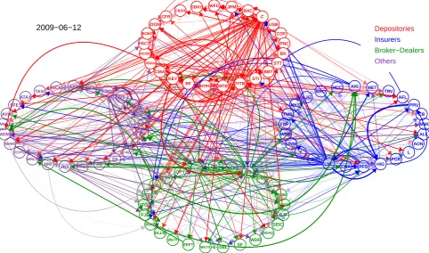
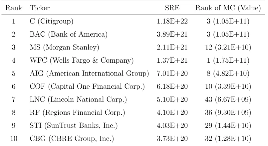
j=1|Db_js_|i|. Figure 3 shows the incoming links for these four groups. The patterns of these four groups are almost identical, i.e. there are more links during the end of 2008 and beginning of 2010, during the middle of 2011 and the end of 2012. Only for group “others”, there are even more links between 2010 and 2012, this maybe because the heterogeneity of this group: AXP (American Express Company) is a credit card com-pany, JLL (Jones Lang LaSalle Incorporated), CBG (CBRE Group, Inc) and AVHI (AV Homes, Inc.) are real estate firms, BEN (Franklin Resources, Inc.), IVZ (Invesco Plc) and AMG (Affiliated Managers Group) are investment management companies, whereas OCN (Ocwen Financial Corporation) and AGM (Federal Agricultural Mortgage Corpora-tion) are mortgage loan companies. While the depositories group (solid line) received on average more risk than the other three groups, the insurance companies (dashed line) are less influenced by the financial crisis. This can be seen as evidence supporting the report of Systemic Risk in Insurance – An analysis of insurance and financial stability published by Geneva Association in 2010 stating that losses in the insurance industry have been only a sixth of those at banks. In contrast to the incoming links the outgoing links in Figure 4 are more volatile. It is not surprising that the depositories sector dominates the others in the outgoing links, i.e. the bank group emits more risk to the system than the other groups. Broker-dealers and others fluctuate very much in the whole period, but they send out less risk compared with banks. And the insurers emit averagely less risk over all periods than the other groups.

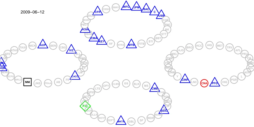
direc-tional connectedness from firmi to the firmj which is defined as follows: DC_js_|i def= |Dbs_j|i|. The network in Figure 5 shows one example of the firm level directional connectedness on 12 June 2009 which was in the financial crisis. There are several links emitted from C (Citigroup) and MS (Morgan Stanley). To make the major connections more clearly, we apply a hard thresholding to omit the small values. That is, the values of absolute deriva-tives smaller than the average of the 100 largest absolute partial derivaderiva-tives are set to be zeros. Figure 6 is the network after the thresholding. We see that there are several strong connections, for example, in violet circle the link from JLL to CBG (as we stated before they are both real estate companies, the connection induced by spillover effects seems reasonable), and in blue circle from PRU (Principal Financial Group) to HIG (Hartford Financial Services Group), note that they are both insurances. Moreover there are also a couple of weak connections from MS (Morgan Stanley) to others. Furthermore, there are a lot of mutual connections, big banks like BAC (Bank of America) and C (Citigroup) in red circle, STT (State Street Corporation) and FITB (Fifth Third Bancorp) in red circle, insurances: LNC (Lincoln National Corporation) and HIG (Hartford Financial Services Group) in blue circle, different groups, e.g. MS (a broker dealer) and KEY (KeyCorp, a big bank). We aggregate the directional connectedness by the sum of absolute value of

b

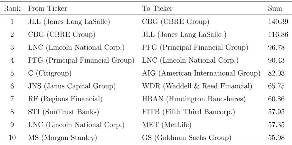
Ds_j|i andDb_is_|j overT = 266 windows. The results for individual firm can be found in Table 3. For WFC (Wells Fargo) the strong incoming links come from STI (SunTrust Banks), C and BAC, the outgoing links go to USB (U.S. Bancorp), STI and CBSH (Commerce Bancshares). We also see some pairs of mutual interacting firms, like BAC and C, AIG (American International Group) and MS. We show the directional connection inτ = 0.95 case as well, the selected firms are mostly different from τ = 0.05 case, which shows that our method can explain the asymmetric effects on the dependency structure at different price levels. See Table 3 for more details. The ranking of the directional connectedness is calculated by the sum of absolute value ofDbs_j|i over windows. The first two strongest mu-tual connections are between JLL and CBG, between LNC and PFG (Principal Financial Group), see Table 4. Secondly, the firm connectedness with respect to incoming links is defined as F C_j,sIN =Pk

i=1|Db_js_|i|. Finally, the firm connectedness with respect to outgoing links is: F C_j,sOU T =Pk

and CLMS (Calamos Asset Management) and JNS (Janus Capital Group) with OUT-link. This is connected with the Global Financial Stability Report (GFSR) of April 2009 which states that the crisis has shown that not only the banks but also other non-bank financial intermediaries can be systemically important and their failure can cause desta-bilizing effects. It also emphasizes that not only the largest financial institutions but also the smaller but interconnected financial institutions are systemically important and

need to be regulated. “Too connected to fail” is an important issue. However, we see that small firms tends to have more connections with small firms, such as AGM (market cap $0.35 billion), which is with the largest sum of incoming links coming from GFIG (market cap. $0.29 billion), LTS (market cap. $0.22 billion), NEWS (market cap.$0.62 billion), OPY (market cap.$0.21 billion) and HBAN (market cap. $5.2 billion). Despite the heavy connections in the system, one would still not consider it as highly systemic risk relevant. Therefore we try to account the three factors in the forthcoming systemic risk analysis: (1) a firm is big enough, (2) a firm is highly connected with other firms, (3) the connected firms are relative large in size. Therefore to identify the systemically important financial institutions, we add a weight of market capitalization in the network.

In addition, based on our network analysis we have the following findings: (1) the con-nections between institutions tend to increase before the financial crisis, (2) the network is characterized by numerous heavy links at the peak of a crisis, (3) the connections be-tween institutions reflected by the absolute value of partial derivatives get weaker as the financial system stabilizes, (4) the incoming links are far less volatile than the outgoing links. Whereas banks dominate both incoming and outgoing links, the insurers are less affected by the financial crisis and exhibit less contribution in terms of risk transmission. The broker-dealer and others are highly volatile with respect to the risk contribution. (5) Several institutions with moderate or small sizes and also some non-bank institutions have higher connectedness, as they are too connected firms. (6) “Too connected” is not a sufficient condition to detect the importance of the firm. To identify the systemically important financial institutions we need to find a measure which combines the concepts “too connected to fail” and “too big to fail”.

during crisis, WFC (Wells Fargo), JPM (J P Morgan) and C (Citigroup) are very fre-quently classified into the same cluster. For Figure 8, we see that the clusters are more widely spreading cross sectors.

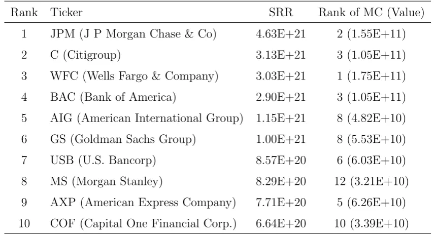
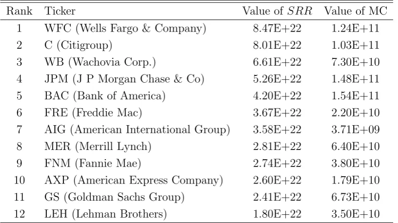
In the third step we provide an exact systemic risk measure for each firm based on their connectedness structure. We consider the market capitalization of each firm as well as its connected firms with incoming or outgoing links, see equation (12) and (13). Ta-ble 7 shows the ranking of the top 10 calculated Systemic Risk Receivers: JPM (J P Morgan), C (Citigroup), WFC (Wells Fargo), BAC (Bank of America), AIG (American International Group), GS (Goldman Sachs), USB (U.S. Bancorp), MS (Morgan Stanley), AXP (American Express Company) and COF (Capital One Financial Corp.). As for the Systemic Risk Emitters, the corresponding ranking is presented in Table 8. Although the market capitalization of LNC and RF are moderate, they are still ranked in the top 10 largest systemic risk emitters list, as they have many strong outgoing links. Compared with the result of global systemically important banks (G-SIBs) published by Financial Stability Board 2012, six of our top ten systemic risk receivers appear in this report: JPM (J P Morgan), C (Citigroup), WFC (Wells Fargo), BAC (Bank of America), GS (Goldman Sachs), MS (Morgan Stanley), whereas four of our top ten systemic risk emit-ters appear in this report: C (Citigroup), BAC (Bank of America), WFC (Wells Fargo & Company) and MS (Morgan Stanley). Also we compare our result with the global sys-temically important insurers (G-SIIs) published by the Financial Stability Board 2013, AIG (American International Group) is present in their list. We also compare with the list of all domestic systemically important banks (D-SIBs) in U.S. published by Board of Governors of the Federal Reserve System 2013, USB (U.S. Bancorp), AXP (American Express), COF (Capital One Financial Corp.), RF (Regions Financial Corp.) and STI (SunTrust Banks, Inc.) are on that list. In total all our top 10 Systemic Risk Receivers and 8 of our top 10 Systemic Risk Emitters are identified as systemically important fi-nancial institutions. In this step, we could identify “too big as well as too connected” firms which need to be well supervised and regulated.

3.3

.

Model Validation

3.3.1. Comparison with linear models

of estimated VaRs do not have violation, the CaViaR test for VaR can not be performed. In step 2 we apply the SIM with variable selection to calculate CoVaR. We also compare our results with linear quantile LASSO models in this step to justify the necessity of having a nonlinear model. The benchmark linear LASSO model is written as follows:

Xj,t =αj|Rj +βjL|Rj> Rj,t+εj,t, (14)

\

CoVaRL_j|Rj,t,τe

def

= α_bj| e Rj+βb

L> j|Rje

e

Rj,t, (15)

whereαj|Rj is a constant term, Rj,t,X−j,t,Bj,t−1,VaRd−j,t,τ andRe_j,t are defined in section

2.3. The parameters βL j|Rj

def

= {βL

j|−j, βjL|M, βjL|Bj}

>_{, and}

b

βL j|Rj

def

= {βb_jL_|−j, βb_jL_|M, βb_jL_|Bj}> which are estimated by using linear quantile regression with variable selection. Then

\

CoVaRL can be simply calculated.3

Recall that we denote our estimated CoVaR in step 2 asCoVaR\ T EN ET. Now we compare the performance of CoVaR\ T EN ET and CoVaR\ L. In Figure 1 the thinner green line rep-resents the CoVaR\ L of J P Morgan, there is 1 violation during the whole time period of

T = 266, whereas there are 4 violations in the estimated CoVaR\ T EN ET series in Figure 1 (thicker blue line). We apply the CaViaR test proposed by Berkowitz et al. (2011).

While the p-values of CoVaR\ T EN ET in overall period is 0.63, CoVaR\ L is only 0.37. Also in crisis period (from 15 September 2008 to 26 February 2010) CoVaR\ T EN ET performs

better than CoVaR\ L, see Table 9 for more details.

Further, we examine the shape of the link functions in the crisis period as well as in the period of relative financial stability. We find out that for almost all firms in a financial crisis period, the link functions are in most of the windows, non-linear, while in a stable period, the link functions tend to be more linear. Take theCoVaR\ T EN ET for J P Morgan as an example. The left panel of Figure 9 displays the shape of the estimated link function in one window in crisis time and its 95% confidence bands, see Carroll and H¨ardle (1989). In a stable period one observes in some windows the shape of the link function as on the right panel of Figure 9. It confirms Chao et al. (2015)’s results stating that the nonlinear model performs better especially in a financial crisis period. We conclude the outperformance of our method over the linear model conditional on the network effects.

3.3.2. Pre-Crisis analysis

In this part we would like to test whether our model can detect in advance financial firms which had knock-on effects for the financial systems. We consider mainly five financial firms: FNM (Fannie Mae), FRE (Freddie Mac), LEH (Lehman Brothers), MER (Merrill

3_{For simplicity we omit the subscript}

j|Rej,t,τ in CoVaR\

L

j|Rej,t,τ, and write CoVaR\

L

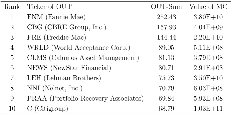
Lynch) and WB (Wachovia Corp.). The weekly historical returns of these firms are available on the CRSP database. The above mentioned exercise has been carried out again with these five firms (a total of 105 firms in this case). The time period is from 7 December 2007 to 12 September 2008 includes 41 estimates in moving windows. Firstly we show the results from step 2, which checks the connectedness of these firms. Table 10 shows the ranking of total incoming links, where FRE receives most incoming links

from other firms, and FNM is ranked as the 4th. From the Table 11 it can be seen that the firm with the strongest outgoing links is FNM. Moreover FRE is ranked as the third one, and LEH is ranked in the 7th place. Table 12 presents the direct incoming links and outgoing links in terms of other firms. Besides, FRE and FNM is the most connected pair, they send risk to each other. FNM dominates the incoming link tables, which can also be confirmed in Table 10. According to the selected variables in step 2, we perform the methodology in step 3. Table 13 shows the ranking of the systemic risk receivers according to our SRR values, where WB is third largest risk receiver, FRE is ranked as the sixth, AIG, MER, FNM follow subsequently, and LEH is ranked as the 12th. The systemic risk emitters according to our SRE values are presented in Table 14. We see that FNM is the biggest risk emitter, WB is the third one, FRE and LEH are 4th and 5th risk transmitters and the ranking of MER is 8th. In summary, all these five firms are identified as systemically important institutions which shows the validation of our methodology. Finally, we compare our ranking of systemic risk emitters in Table 14 with Hautsch et al. (2015) and Brownlees and Engle (2015). In the pre-crisis results of Hautsch et al. (2015), they involve five firms in the case study, i.e. AIG, FNM, FRE, LEH and MER. MER is not in their top ten list, whereas we did not identify AIG in our top ten list. Compared with the pre-crisis results with Brownlees and Engle (2015), where the firm Bear Stearns is also involved in their analysis. Their rankings of the aforementioned five firms between 2007 and 2008 are very similar with ours.

4

.

Conclusion

In this paper we propose TENET based on a semiparametric quantile regression frame-work to assess the systemic importance of financial institutions conditional to their market capitalization and interconnectedness in tails. The semiparametric model allows for more flexible modeling of the relationship between the variables. This is especially justified in a (ultra) high-dimensional setting when the assumption of linearity is not likely to hold. In order to face these challenges statistically we estimate a SIM in a generalized quantile regression framework while simultaneously performing variable selection. (Ultra) high dimensional setting allows us to include more variables into the analysis.

a financial crisis, and a network-based measure reflecting the connectivity. Moreover, by including more variables into the analysis we can investigate the overall performance of different financial sectors, depositories, insurance, broker-dealers, and others. Estimation results show a relatively high connectivity of depository industry in the financial crisis. We also observe strong non-linear relationships between the variables, especially, in the period of relative financial instability. The Systemic Risk Receivers and Systemic Risk

5

.

Appendix A: Statistical Methodology

Let us denote Xt ∈Rp aspdimensional variables Rj,t in (9),pcan be very large, namely

of an exponential rate. We also drop the subscripts of the coefficients βj|Rj, as we focus

on one regression. The SIM of (9) is then rewritten as:

Yt =g(Xt>β ∗

) +εt, (16)

where {Xt, εt} are strong mixing processes, g(·): R1 → R1 is an unknown smooth link

function,β∗ is the vector of index parameters. RegressorsXt can be the lagged variables

of Yt. For the identification, we assume that kβ∗k2 = 1, and the first component of β∗ is

positive. We assume that there are q non-zero components in β∗.

Note that (16) can be formulated in a location model and identified in a quasi maximum likelihood framework: the direction β∗ (for known g(·)) is the solution of

min

β Eρτ{Yt−g(X >

t β)}, (17)

with loss function

ρτ(u) =τ u1(u >0) + (1−τ)u1(u <0), (18)

E[ψτ{Yt−g(Xt>β ∗_)}|X

t] = 0 a.s.

whereψτ(·) is the derivative (a subgradient) ofρτ(·) . It can be reformulated asF_εt−|1Xt(τ) =

0.

The model is similar to the location scale model considered in Franke et al. (2014). Note that it may be extended to a quantile AR-ARCH type of single index model,

Yt=g(Xt>β ∗

) +σ(X_t>γ∗)εt (19)

ˆ

βτ,gˆ(·)

def

= arg min

β,g(·)−Ln(β, g(·))

= arg min

β,g(·)n

−1

n

X

j=1

n

X

t=1

ρτ

Xt−g(β>Xj)−g0(β>Xj)Xtj>β ωtj(β)

+

p

X

l=1

γλ(|βl|), (20)

where ωtj(β)

def

= Kh(X

> tjβ)

Pn

t=1Kh(Xtj>β)

, Kh(·) = h−1K(·/h), K(·) is a kernel e.g. Gaussian

kernel, h is a bandwidth and Ln(β, g(·)) is defined as −n−1 n

P

j=1

n

P

t=1

ρτ

Xt −g(β>Xj)−

g0(β>Xj)Xtj>β ωtj(β) +

Pp

l=1γλ(|βl|). Since the data is not equally spaced we choose a

bandwidthhbased on k-nearest neighbour procedure (See H¨ardle et al. (2004) and Carroll and H¨ardle (1989)). The optimalk, number of neighbours, are selected based on a cross-validation criterion. The implementation involves an iteration between estimatingβ∗ and

g(·), with a consistent initial estimate for β∗, Wu et al. (2010). Xtj = Xt−Xj, θ ≥ 0,

and γλ(t) is some non-decreasing function concave for t ∈ [0,+∞) with a continuous

derivative on (0,+∞). Please note that this MACE functional (with respect to g(·)) (20) is in fact only a finite dimensional optimization problem since the minimum over

g(·) is to be determined at aj = g(β>Xj), bj = g0(β>Xj). There are several approaches

for the choice of the penalty function. These approaches can be classified based on the properties desired for an optimal penalty function, namely, unbiasedness, sparsity and continuity. The L1 penalty approach known as least absolute shrinkage and selection

operator (LASSO) is proposed for mean regression by Tibshirani (1996). Numerous studies further adapt LASSO to a quantile regression framework, Yu et al. (2003), Li and Zhu (2008), Belloni and Chernozhukov (2011), among others. While achieving sparsity the L1-norm penalty tends to over-penalize the large coefficients as the LASSO penalty

increases linearly in the magnitude of its argument, and, thus, may introduce bias to estimation. As a remedy to this problem the adaptive LASSO estimation procedure was proposed (Zou (2006); Zheng et al. (2013)). Another approach to alleviate the LASSO bias was proposed by Fan and Li (2001) known as Smoothly Clipped Absolute Deviation (SCAD):

γλ(t) =

  

 

λ|t| for |t| ≤λ,

−(t2−2aλ|t|+λ2)/2(a−1) for λ <|t| ≤aλ,

(a+ 1)λ2/2 for |t|> aλ,

As for selecting λ, there are two common ways: data-driven generalized cross-validation criterion (GCV) and likelihood-based Schwartz, or Bayesian information criterion-type criteria (SIC, or BIC), Schwarz (1978); Koenker et al. (1994), and their further modifi-cations. The most commonly used criterion is GCV, however, it has been shown that it leads to an overfitted model. Therefore, we employ a modified BIC-type model selection criteria proposed by Wang et al. (2007) and use GCV criterion only to verify whether

GCV and BIC diverge significantly. We need to introduce some more notation to present our theoretical results.

Define ˆβτ

def

= ( ˆβ_τ>₍₁₎,βˆ_τ>₍₂₎)> as the estimator for β∗ def= (β₍₁₎∗>, β₍₂₎∗>)> attained by the loss in (20). Here ˆβτ(1) and ˆβτ(2) refer to the first q components and the remaining p−q

components of ˆβτ respectively. The same notional logic applies to β∗. For Xt, X(1)t

corresponds toβ₍₁₎∗> and X(0)t corresponds toβ(2)∗>. If in the iterations, we have the initial

estimator ˆβ₍₁₎(0) as a pn/q consistent one for β₍₁₎∗ , we will obtain, with a very high probability, an oracle estimator of the following type, say ˜βτ = ( ˜βτ>(1),0

>

)>, since the

oracle knows the true model M∗

def

= {l :β_l∗ 6= 0}. The following theorem shows that the penalized estimator enjoys the oracle property. Define ˆβ0 ∈Rp as the minimizer with the same loss in (20) but within subspace {β ∈Rp :βMc

∗ =0}.

With all the above definitions and conditions, see Appendix, we present the following theorems.

THEOREM 5.1. Under Conditions 1-7, the estimators βˆ0 _{and β}ˆ

τ exist and coincide

on a set with probability tending to 1. Moreover,

P( ˆβ0 = ˆβτ)≥1−(p−q) exp(−C0nα) (21)

for a positive constant C0, where βˆ0 _{is the “ideal” estimator with non-zero elements}

correctly specified.

This theorem implies the sign consistency.

THEOREM 5.2. Under Conditions 1-7, we have

kβˆτ(1)−β(1)∗ k=Op{(Dn+n−1/2) √

q} (22)

For any unit vector b in Rq, we have

b>C₀₍₁₎1/2C₁₍₁₎−1/2C₀₍₁₎1/2√n( ˆβτ(1)−β(1)∗ )

L

−→N(0,1) (23)

where C1(1) def

= E{E{ψ_τ2(εt)|Zt}[g0(Zt)]2[E(X(1)t|Zt) − X(1)t][E(X(1)t|Zt) − X(1)t]>}, and C0(1)

def

E(X(1)t|Zt) denotes a p×1vector, and Zt

def

= X_t>β∗, ψτ(εt) is a choice of the subgradient

of ρτ(εt) and

σ_τ2 def= E[ψτ(εt)]2/[∂Eψτ(εt)]2, where

∂Eψτ(·)|Zt=

∂Eψτ(εt−v)2|Zt ∂v2

v=0. (24)

Let us now look at the distribution of ˆg(·) and ˆg0(·), estimators ofg(·), g0(·).

THEOREM 5.3. Under Conditions 1-7, for any interior point z =x>β∗, fZ(z) is the

density of Zt, t= 1, . . . , n, if nh3 → ∞ and h→0, we have

√

nhpfZ(z)/(ν0σ2τ)

b

g(x>βb)−g(x>β∗)− 1 2h

2_g00

(x>β∗)µ2∂Eψτ εt

L

−→N(0, 1),

Also, we have

√ nh3

q

{fZ(z)µ22}/(ν2στ2)

n b

g0_(x>

b

β)−g0(x>β∗)o−→L N(0, 1).

The dependence doesn’t have any impact on the rate of the convergence of our non-parametric link function. As the degree of the dependence is measured by the mixing coefficient, it is weak enough such that Condition 7 is satisfied. In fact we assume an exponential decaying rate here, which implies the (A.4) in Kong et al. (2010).

6

.

Appendix B: Proof

Condition 1. The kernel K(·) is a continuous symmetric function. The link function

g(·)∈C2_{, let µ}

j

def

= R

uj_{K(u)du and ν} j

def

= R

uj_K2_{(u)du, j = 0,1,2.}

Condition 2. The derivative (or a subgradient) of ρτ(x), satisfies Eψτ(εt) = 0 and

inf|v|≤c∂Eψτ(εt −v) = C1 where ∂Eψτ(εt −v) is the partial derivative with respect

tov, andC1 is a constant.

Condition 3. The density fZ(z) of Zt = β∗>Xt is bounded with bounded absolute

con-tinuous first-order derivatives on its support. Assume E{ψτ(εt|Xt)} = 0 a.s., which

means for a quantile loss we have F_εt−_|1_Xt(τ) = 0. Let X(1)t denote the sub-vector of

Xt consisting of its first q elements. Let Zt

def

= X_t>β∗ and Ztj

def

= Zt −Zj . Define C1(1)

def

= E{E{ψ2_τ(εt)|Zt}[g0(Zt)]2[E(X(1)t|Zt)−X(1)t][E(X(1)t|Zt)−X(1)t]>}, and C0(1) def

=

E{∂Eψτ(εt)|Zt}{[g0(Zt)]2(E(X(1)t|Zt)−X(1)t)(E(X(1)t|Zt)−X(1)t)}>, and the matrixC1(1)

satisfies 0< L1 ≤λmin(C0(1))≤ λmax(C0(1))≤L2 <∞ for positive constants L1 and L2.

A constant c0 > 0 exists such that Pn_t=1{kX(1)tk/

√

n}2+c0 _{→ 0, with 0 < c}

0 < 1.

vtj

def

(kβ−β∗k ≤ C3), let X(1)tj denote the subvector of Xtj consisting of its first q

compo-nents, X(0)tj denote the subvector of Xtj consisting of its first p−q components:

kX

t

X

j

X(0)tjωtjX(1)>tj∂Eψτ(vtj)k2,∞=Op(n1−α1).

Condition 4. The penalty parameter λ is chosen such that λ = O(n−1/2_{), with D}

n

def

= max{dl : l ∈ M∗} = O(nα1−α2/2λ) = O(n−1/2), dl

def

= γλ(|βl∗|), M∗ = {l : βl∗ 6= 0} be

the true model. Furthermore assume qh→0 and h−1p

q/n=O(1) as n goes to infinity, q = O(nα2_{), p =} O{_exp(nδ₎}_{, nh}3 → ∞ _{and h} → _{0. Also, 0 < δ < α < α}

2/2 < 1/2,

α2/2< α1 <1.

Condition 5. The error term εt satisfies Var(εt) < ∞. Assume that for any integer m= 1,· · · ,∞

sup

t

Eψ_τm(εt)/m!

≤s0Mm

sup

t

Eψ_τm(xtj)/m!

≤s0Mm

where s0 and M are constants, and ψτ(·) is the derivative (a subgradient) ofρτ(·).

Condition 6. The conditional density function f(εt|Zt = z) is bounded and absolutely

continuously differentiable.

Conditions 7. {Xtj, εt}tt==∞−∞ is a strong mixing process for any j. Moreover, let m1 and m2 be constants, positive constantscm1andcm2 exists such that theα−mixing coefficient

for every j ∈ {1,· · · , p},

α(l)≤exp(−cm1lcm2), (25)

where cm2 >2α.

Recall (20) and ˆβ0 as the minimizer with the loss

˜

Ln(β)

def

=

n

X

j=1

n

X

t=1

ρτ Yt−a∗j −b ∗ jX

> tjβ

ωtj(β∗) +n p

X

l=1

dl|βl|,

but within the subspace {β ∈Rp :βMc

∗ = 0}, and a

∗

j =g(β∗>Xj), b∗j = g0(β∗>Xj). The

following lemma assures the consistency of ˆβ0,

LEMMA 6.1. Under Conditions 1-7, recall dj =γλ |βj∗|

, we have that

kβˆ0−β∗k=Op

p

q/n+kd(1)k

(26)

where d(1) is the subvector of d= (d1,· · · , dp)> which contains q elements corresponding

PROOF. Note that the last p−q elements of both ˆβ0 _{and β}∗ _{are zero, so it is sufficient}

to prove kβˆ0

(1)−β

∗

(1)k=Op

p

q/n+kd(1)k

.

Following Fan et al. (2013), it is not hard to prove that for γn=O(1):

P

inf

kuk=1

_˜

Ln(β(1)∗ +γnu, 0)>L˜n(β∗)

→1.

Then a minimizer inside the ball exists {β(1) : kβ(1)−β(1)∗ k ≤ γn}. Construct γn → 0

so that for a sufficiently large constant B0: γn > B0 ·

p

q/n+kd(1)k

. Then by the local convexity of ˜Ln(β(1),0) near β(1)∗ , a unique minimizer exists inside the ball {β(1) :

kβ(1)−β(1)∗ k ≤γn} with probability tending to 1.

Recall that Xt = (X(1)t, X(0)t) andM∗ = {1, . . . , q} is the set of indices at which β are

non-zero.

Lemma 1 shows the consistency of ˆβ0, and we need to show further that ˆβ0 is the unique minimizer inRp on a set with probability tending to 1.

LEMMA 6.2. Under conditions 1-7, minimizing the loss function L˜n(β) has a unique

global minimizerβˆτ = ( ˆβτ>(1),βˆ

> τ(2))

> _{= ( ˆβ}> τ(1),0

>₎>_{, if and only if on a set with probability}

tending to 1,

n

X

j=1

n

X

t=1

ψτ Yt−ˆaj −ˆbjXtj>βˆτ

_ˆ

bjX(1)tjωtj(β∗) +nd(1)◦sign( ˆβτ) = 0 (27)

kz( ˆβτ)k∞≤n, (28)

where

z( ˆβτ)

def

= d−₍₀₎1◦

n X

j=1

n

X

t=1

b∗_jψτ Yt−a∗j −b ∗ jX

> tjβˆτ

X(0)tjωtj( ˆβτ)

(29)

where ◦ stands for multiplication element-wise.

PROOF. According to the definition of ˆβτ, it is clear that ˆβ(1) already satisfies condition

(27). Therefore we only need to verify condition (28). To prove (28), a bound for

n

X

i=1

n

X

i=1

b∗_jψτ Yi−a∗j −b ∗ jX

> ijβ

∗

ωijX(0)ij (30)

is needed, note that to be consistent with notations forU− statistics we use j instead of

t within this proof. Define the following kernel function

hd(Xi, a∗j, b ∗

j, Yi, Xj, a∗i, b ∗ i, Yj)

= n 2

b∗_jψτ Yi−a∗j −b ∗ jX

> ijβ

∗

ωijX(0)ij +b∗iψτ Yj −a∗i −b ∗ iX

> ijβ

∗

ωjiX(0)ji

where {.}d denotes thedth element of a vector,d= 1, . . . , p−q.

According to Borisov and Volodko (2009), based on Condition 5:

DefineUn,d

def

= _n(n1₋₁₎P

1≤i<j≤nhd(Xi, a ∗ j, b

∗

j, Yi, Xj, a∗i, b ∗

i, Yj) as theU−statistics for (30).

We have, with sufficient large cm2 in Condition 7.

P{|Un,d−EUn,d|> ε} ≤ cm3exp(cm5ε/(cm3+cm4ε1/2n−1/2))

where cm3, cm4, cm5 are constants. Moreover, let ε=O(n1/2+α) and m6 be a constant, as

α <1/2, we can further have,

P({|Un,d−EUn,d|> ε}) ≤ cm3exp(−cm6ε/2),

Define

Fn,d

def

= (n)−1

n

X

i=1

n

X

j=1

bjψτ Yi−a∗j −b ∗ jX

> ijβ

∗

ωijX(0)ij,

also it is not hard to derive that Un,d=Fn,dn/(n−1).

It then follows that

P(|Fn,d−EFn,d|> ε) = P(|Un,d−EUn,d|(n−1)/n > ε) ≤ 2 exp −Cnα+1/2

DefineAn={kFn−EFnk∞≤ε}, thus

P(An)≥1− p−q

X

d=1

P(|Fn,d−EFn,d|> ε)≥1−2(p−q) exp −Cnα+1/2

.

Finally we get that on the set An,

kz( ˆβ0)k∞ ≤ kd−M1c

∗◦Fnk∞+kd

−1

Mc

∗◦

n

X

i=1

n

X

j=1

bj

ψτ Yt−a∗j −b ∗ jX

> ijβˆ

0

−ψτ Yt−a∗j −b ∗ jX

> ijβ

∗

ωijX(0)ijk∞

≤ O(n1/2+α/λ+kd−_M1c

∗ ◦

n

X

i=1

n

X

j=1

∂Eψτ(vij)bjX(1)>ij( ˆβ(1)−β(1)∗ )ωtjX(0)ijk∞),

where vij is betweenYi−a∗j −b ∗ jX

> ijβ

∗ _{and Y}

i−a∗j −b ∗ jX

>

ijβˆ0. From Lemma 1,

kβˆ0−β₍₁₎∗ k2 =Op

kd(1)k+

√ q/√n

.

ChoosingkP

i

P

jX(0)ijωijX >

(1)ij∂Eψτ(vij)k2,∞ =Op(n

n−1/2+α2/2_{, 0< α}

2 <1, kd(1)k=O(

√

qDn) = O(nα2/2Dn)

n−1kz( ˆβ0)k∞ = O{n−1λ−1(n1/2+α+n1−α1 √

q/√n+kd(1)kn1−α1)}

= O(n−α2/2+α_+n−α1 _+n−α1+α2/2_D

n/λ),

conditions 4ensuresDn =O(nα1−α2/2λ), and let 0 < δ < α < α2/2<1/2,α2/2< α1 <1,

with rate p=O{exp(nδ_{)}, then (n)}−1_{kz( ˆβ}0_)k

∞ =Op(1).

Proof of Theorem 1 . The results follows from Lemma 1 and 2.

Proof of Theorem 2. By Theorem 1, ˆβτ(1) = β(1) almost surely. It then follows from

Lemma 2 that

kβˆτ(1)−β(1)∗ k=Op{(Dn+n−1/2) √

q}.

● ●●●● ● ● ●● ● ●● ●● ● ● ● ● ● ● ● ● ● ● ● ● ● ● ● ● ● ● ● ● ●● ● ●●●● ● ● ● ●●● ● ●● ● ● ● ● ●● ● ● ● ●●● ● ● ● ● ● ● ● ● ● ●● ● ● ● ● ● ● ● ●● ● ● ● ●● ● ●●●●● ● ●● ● ●● ● ● ●●●●●● ● ● ● ● ● ●●●● ● ●●●● ●●●● ●●●●●● ●●● ● ● ●●●● ● ●● ● ●●●● ● ● ●● ● ●●● ●● ● ● ●●●● ●● ●● ●●●●●●●●● ● ● ●●●●●● ● ● ●● ● ● ●●● ● ● ● ● ● ●●●● ● ● ● ●● ● ● ● ● ● ● ●● ●●● ● ● ● ● ● ●● ●●● ● ● ●● ● ● ●●● ● ● ● ● ● ● ● ●●● ●● ●● ● ●● ● ● ●● ● ●●●● ●●

2008 2009 2010 2011 2012 2013

−1.0

−0.5

0.0

0.5

1.0

Figure 1: log return of J P Morgan (black points),VaR (thinner red line),d CoVaR\

T EN ET

(thicker blue

line), andCoVaR\ L (thinner green line) for J P Morgan,τ= 0.05, window sizen= 48,T = 266.

● ● ● ● ● ● ● ● ● ● ●● ● ● ● ● ● ● ● ● ● ● ●●● ● ● ● ● ● ● ● ● ● ● ●● ● ● ● ● ● ● ● ● ● ● ● ●● ● ● ● ● ● ● ● ●● ● ●● ● ● ●●● ●●●●● ● ● ● ●●● ●● ● ●● ●● ●●●● ●● ● ● ●● ● ●●● ●● ●● ● ● ● ●● ● ● ● ●●● ● ● ● ● ● ●●● ● ● ● ● ● ● ● ● ●●● ● ● ● ● ● ● ● ● ● ● ●●●●● ●● ● ● ● ● ● ●●● ● ● ● ● ● ●●● ● ● ●●● ● ● ● ● ● ● ● ● ●● ● ● ● ● ● ● ● ● ● ●● ● ● ● ● ● ● ● ● ● ● ●●● ●● ● ●●●● ● ● ● ● ● ●●●●● ● ●●● ● ● ● ● ●● ● ●● ●●● ●● ●● ● ● ● ● ● ● ● ●●● ● ●● ● ● ● ● ● ● ● ● ●● ●

2008 2009 2010 2011 2012 2013

0.0 0.2 0.4 0.6 0.8 1.0

2008 2009 2010 2011 2012 2013

0

5

10

15

20

25

Figure 3: Incoming links for four industry groups. Depositories: solid red line, Insurances: dashed blue line, Broker-Dealers: dotted green line, Others: dash-dot violet line. τ= 0.05, window sizen= 48,

T = 266.

2008 2009 2010 2011 2012 2013

0

5

10

15

20

25

Figure 4: Outgoing links for four industry groups. Depositories: solid red line, Insurances: dashed blue line, Broker-Dealers: dotted green line, Others: dash-dot violet line. τ= 0.05, window sizen= 48,

WFC JPM BAC C USB COF PNC BK STT BBT STI FITB MTB NTRS RF KEY CMA HBAN HCBK PBCT BOKF ZION CFR CBSH SBNY AIG MET TRV AFL PRU CB MMC ALL AON L PGR HIG PFG CNA LNC CINF Y UNM WRB FNF TMK MKL AJG BRO HCC GS BLK MS CME SCHW TROW AMTD RJF SEIC NDAQ WDR SF GBL MKTX EEFT WETF DLLR BGCP PJC ITG INTL GFIG LTS OPY CLMS AXP BEN CBG IVZ JLL AMG OCN EV LM CACC FII AB PRAA JNS NNI WRLD ECPG NEWS AGM WHG AVHI SFE ATAX TAXI NICK 2009−06−12 Depositories Insurers Broker−Dealers Others

Figure 5: A circular network representation of a weighted adjacency matrix without the thresholding. Depositories: clockwise 25 firms from WFC to SBNY (upper red), Insurance: clockwise 25 firms from AIG to HCC (right blue), Broker-Dealers: clockwise 25 firms from GS to CLMS (lower green), Others: clockwise 25 firms from AXP to NICK (left violet), date: 20090612,τ= 0.05, window sizen= 48.

WFC JPM BAC C USB COF PNC BK STT BBT STI FITB MTB NTRS RF KEY CMA HBAN HCBK PBCT BOKF ZION CFR CBSH SBNY AIG _MET TRV AFL PRU CB MMC ALL AON L PGR HIG PFG CNA LNC CINF Y UNM WRB FNF TMK MKL AJG BRO HCC GS BLK MS CME SCHW TROW AMTD RJF SEIC NDAQ WDR SF GBL MKTX EEFT WETF DLLR BGCP PJC ITG INTL GFIG LTS OPY CLMS AXP _BEN CBG IVZ JLL AMG OCN EV LM CACC FII AB PRAA JNS NNI WRLD ECPG NEWS AGM WHG AVHI SFE ATAX TAXI NICK 2009−06−12 Depositories Insurers Broker−Dealers Others

WFC JPM BAC C USB COF PNC BK STT BBT STI FITB MTB NTRS RF KEY CMA HBAN HCBK PBCT BOKF ZION CFR CBSH SBNY AIG MET TRV AFL PRU CB MMC ALL AON L PGR HIG PFG CNA LNC CINF Y UNM WRB FNF TMK MKL AJG BRO HCC GS BLK MS CME SCHW TROW AMTD RJF SEIC NDAQ WDR SF GBL MKTX EEFT WETF DLLR BGCP PJC ITG INTL GFIG LTS OPY CLMS AXP BEN CBG IVZ JLL AMG OCN EV LM CACC FII AB PRAA JNS NNI WRLD ECPG NEWS AGM WHG AVHI SFE ATAXTAXI NICK 2009−06−12

Figure 7: A circular network representation of an unweighted adjacency matrix (1 and 0 representation of this matrix) without thresholding. Green, blue, red, black represent four different risk clusters, and grey represents unconnected firm. Date: 20090612,τ= 0.05, window sizen= 48.

WFC JPM BAC C USB COF PNC BK STT BBT STI FITB MTB NTRS RF KEY CMA HBAN HCBK PBCT BOKF ZION CFR CBSH SBNY AIG MET TRV AFL PRU CB MMC ALL AON L PGR HIG PFG CNA LNC CINF Y UNM WRB FNF TMK MKL AJG BRO HCC GS BLK MS CME SCHW TROW AMTD RJF SEIC NDAQ WDR SF GBL MKTX EEFT WETF DLLR BGCP PJC ITG INTL GFIG LTS OPY CLMS AXP BEN CBG IVZ JLL AMG OCN EV LM CACC FII AB PRAA JNS NNI WRLD ECPG NEWS AGM WHG AVHI SFE ATAXTAXI NICK 2012−08−10