Optimization methods for deadbeat control design: a state space approach

City, University of London Institutional Repository

Citation

:

This is the accepted version of the paper.

This version of the publication may differ from the final published

version.

Permanent repository link:

Link to published version

:

Copyright and reuse:

City Research Online aims to make research

outputs of City, University of London available to a wider audience.

Copyright and Moral Rights remain with the author(s) and/or copyright

holders. URLs from City Research Online may be freely distributed and

linked to.

1

Optimization methods for deadbeat control

design: A state space approach

Author:

Somayeh Malekpoor

Thesis submitted as part of the requirement for the degree of

Doctor of philosophy

City University London

School of Mathematics, Computer Science & Engineering

2

Content

List of figures ………. 5

Acknowledgement ………. 8

Abstract ……….. 9

Notation ………. 10

Symbols ……… ..14

Abbreviations ……… 15

Chapter 1 Introduction ……… 17

Chapter 2 The general framework and preliminaries ……….. 30

2.1 Introduction ……….. 30

2.2 Linear fractional transformation (LFT) ……… 30

2.3 The general framework ………. 32

2.4 Internal stability of the LFT ……….. 34

2.5 Coprime factorization and internal stability ………..37

2.6 Parameterization of all stabilizing controllers ………...41

2.7 State space realization of coprime factors and solutions to the Bezout identities ………..46

2.8 Conclusion ……… 49

Chapter 3 Deadbeat controller design; state space and polynomial approaches ………... 52

3.1 Introduction ………...52

3.2 State deadbeat controller- Definition ………53

3.3 State deadbeat controller- Dynamic approach ………..54

3.4 State deadbeat controller- Spectral approach ………60

3.5 State deadbeat controller- Algebraic or transfer function approach ………..62

3.5.1 Sequences, polynomials, and classifications ………..63

3

3.5.3 Sequential description of discrete time systems ……….71

3.5.4 Deadbeat controller synthesis in an algebraic framework ………..77

3.6 A numerical algorithm for eigenvalue assignment ………86

3.7 Conclusion ……….93

Chapter 4 Deadbeat controller design with time domain constraints ………..96

4.1 Introduction ………...96

4.2 Input-output description of deadbeat systems ………...97

4.3 Transient response and time domain constraints ………...98

4.4 Linear Programming (LP) ……….102

4.5 Deadbeat controller design with time domain constraints using linear programming ………104

4.6 Time domain constraints in LQG framework ………...108

4.7 Deadbeat controller design with LQG performance criteria ……….113

4.8 Conclusion ……….124

Chapter 5 Robust pole placement, LMI approach ……….126

5.1 Introduction ………... 126

5.2 System uncertainty and its classifications ……….127

5.3 Investigating the sensitivity of eigenvalues to perturbations ……… 130

5.4 Quadratic stability ………. 132

5.5 Quadratic stability of continuous time systems with structured norm-bounded parametric uncertainty entering the state matrix ……… 135

5.6 Quadratic stability of continuous time systems with structured norm-bounded parametric uncertainty entering both the state and input matrices ……… 139

5.7 Quadratic 𝒟-stability of continuous time systems with structured norm-bounded parametric uncertainty entering the state matrix ……… 142

4

5.9 Quadratic stability of discrete time systems with

structured norm-bounded parametric uncertainty ………. 147

5.10 Quadratic 𝒟-stability of discrete time systems with structured norm-bounded parametric uncertainty when 𝒟 is a circular region ………... 150

5.11 Robust deadbeat controller ………. 154

5.12 Conclusion ……….. 161

Chapter 6 Deadbeat controller design with 𝑯∞ norm minimization constraint; The LMI approach ……….. 163

6.1 Introduction ………...163

6.2 The 𝐻_∞ norm ……… 163

6.3 The 𝐻∞ control problem formulation and its motivations ………166

6.4 Approaches to solve the 𝐻_∞ optimization problem ………..167

6.5 Synthesis of deadbeat controller subject to 𝐻_∞ norm constraint ………..173

6.6 Conclusion ………179

Chapter 7 Conclusion ………... 180

5

List of Figures

Figure 2.2.1 (a) The lower and (b) the upper LFT

Figure 2.3.1 The general framework

Figure 2.4.1 Setup for internal stability definition

Figure 2.4.2 Equivalent diagram to analyse internal stability

Figure 2.6.1 (a) 𝑄-parameterization as modification to nominal controller (b) Closed-loop configuration for the class of all stabilizing controllers

Figure 2.7.1 Interpretation of 𝑄-parameterization for estimated state feedback 𝐾_𝑠

Figure 3.5.4.1 The unity feedback configuration

Figure 4.4.1 The geometric interpretation of an LP

Figure 4.5.1 LFT framework

Figure 4.5.2 LFT framework with 𝐿 channels of exogenous inputs and regulated outputs

Figure 4.7.1 Model structure of an one-storey building

Figure 4.7.2 The electrical model of the actuator

Figure 4.7.3 The generalized regulator

Figure 4.7.4 Discrete model

6

Figure 4.7.6 The control input 𝑢

Figure 4.7.7 First floor acceleration- open-loop system

Figure 4.7.8 First floor acceleration- LQR design

Figure 4.7.9 First floor acceleration- deadbeat control

Figure 4.7.10 Deadbeat control input

Figure 5.2.1 The general configuration for robust controller synthesis

Figure 5.2.2 The 𝑁∆-structure for robust analysis

Figure 5.5.1 Closed-loop feedback interconnection of the system (5.4.3) and the uncertainty characterized in (5.4.4) with nonzero feed-through matrix 𝐿 (as in (5.4.7))

Figure 5.6.1 Closed-loop feedback configuration of perturbed system (5.5.5) with state feedback

Figure 5.11.1 The electric equivalent circuit of the armature and the free-body diagram of the rotor

Figure 5.11.2 The eigenvalue locus of 𝐴𝑑 + 𝐵𝑑𝐹

Figure 5.11.3 The eigenvalue locus of 𝐴_𝑑 + 𝐻𝐶_𝑑

Figure 6.2.1 The equivalent representation of the general framework of the figure 2.2.1

Figure 6.4.1 Model-matching problem illustration

7

Figure 6.5.2 The equivalent lower LFT configuration of figure 6.5.1

8

Acknowledgement

Foremost, I would like to express my deepest appreciation to my first supervisor Professor George Halikias, for his continued support and patience he has shown during the past few years it has taken me to finalize this thesis. His scholarship and hard work have set an example I hope to match someday.

A special gratitude toward my second supervisor Dr Stathis Milonidis for his motivation and support. His guidance and helpful suggestions have served me well and I owe him my sincere appreciation.

Furthermore, I gratefully acknowledge the funding source, the School of Mathematics, Computer Science and Engineering (City University London). My special thanks goes to Professor Nicholas Karcanias for his kind support, especially at the beginning of my work.

The best and worst moments of my doctoral have been shared with my friends at the School of Mathematics, Computer Science and Engineering. You will always remain dear to me.

9

Abstract

This thesis addresses the synthesis problem of state deadbeat regulator using state space techniques. Deadbeat control is a linear control strategy in discrete time systems and consists of driving the system from any arbitrary initial state to a desired final state in finite number of time steps.

Having described the framework for development of the thesis which is in the form of a lower linear-fractional transformation (LFT), the conditions for internal stability based on the notion of coprime factorization over the set of proper and stable transfer matrices, namely ℝ𝐻_∞, is discussed. This leads to the derivation of the class of all stabilizing linear controllers, which are parameterized affinely in terms of a stable but otherwise free parameter 𝑄, usually known as the 𝑄-parameterization. In this work, the classical 𝑄 -parameterization is generalized to deliver a -parameterization for the family of deadbeat regulators.

Time response characteristics of the deadbeat system are investigated. In particular, the deadbeat regulator design problem in which the system must satisfy time domain specifications and minimize a quadratic (LQG-type) performance criterion is examined. It is shown that the attained parameterization for deadbeat controllers leads to the formulation of the synthesis problem in a quadratic programming framework with 𝑄

regarded as the design variable. The equivalent formulation of this objective as a quadratic integral in the frequency domain provides the means for shaping the frequency-response characteristics of the system. Using the LMI characterization of the standard 𝐻∞

problem, a new scheme for shaping the system frequency response characteristics by minimizing the infinity norm of an appropriate closed-loop transfer function is introduced. As shown, the derived parameterization of deadbeat compensators simplifies considerably the formulation and solution of this problem.

10

Notation

ℝ𝐻_∞ Set of proper and stable rational matrices

𝑋𝑇 Transpose of the matrix 𝑋

ℱ𝑙(. , . ) Lower LFT

ℱ_𝑢(. , . ) Upper LFT

𝐶_𝑙 Composition of two LFTs

𝑅𝑛×𝑚 Set of 𝑛 × 𝑚 matrices whose elements all belong to 𝑅

𝐾_𝑠 Nominal (central) controller in the set of admissible controllers

ℝ𝑛×𝑚 Set of 𝑛 × 𝑚 real matrices

𝙲 Controllability matrix

𝑆_𝑖 𝑖-th controllable subspace

𝑣 Controllability (reachability) index

ℝ Set of real numbers

ℂ Set of complex numbers

ℤ Set of integers

ℕ Set of natural numbers

ƒ Field

ƒℤ_{, ƒ〈𝘹〉 Formal Laurent series in one indeterminate 𝘹 over ƒ}

𝜏(𝑓) Order of the sequence 𝑓

ƒ [[𝘹]] Formal power series in one indeterminate 𝘹 over ƒ

ƒ [𝘹] Formal polynomials in one indeterminate 𝘹 over the field ƒ

11

ƒ(𝘹) Rational fractions or rational sequences in one indeterminate 𝘹 over ƒ

(Formal rational series in one indeterminate 𝘹 over ƒ)

ƒ(х) Rational functions in ƒ

𝑑 Indeterminate, delay operator

ℝ{𝑑} Set of recurrent sequences with one indeterminate 𝑑 over ℝ

ℝ(𝑑) Set of rational sequences with one indeterminate 𝑑 over ℝ

ℝ𝑜_{(𝑑) Set of causal sequences with one indeterminate 𝑑 over ℝ}

ℝ+_{(𝑑) Set of stable sequences with one indeterminate 𝑑 over ℝ}

ℝ[𝑑] Set of polynomial sequences with one indeterminate 𝑑 over ℝ

ℝ(𝑑) ℝ𝑜_(𝑑) ℝ+(𝑑)

} Corresponding functions over ℝ

ℝ_𝑙𝑚(𝑑) ℝ_𝑙𝑚𝑜 (𝑑) ℝ_𝑙𝑚+ (𝑑)

} Corresponding sequential matrices

𝔻 Closed unit disc in the complex plane

𝑧 The advance shift operator (𝑧 = 𝑑−1₎

𝛿_𝓂𝑓(𝐺) Number of finite poles of the rational matrix 𝐺

𝛿_𝓂∞_{(𝐺) Number of infinite poles of the rational matrix 𝐺}

𝛿_𝑚(𝐺) McMillan degree of the rational matrix 𝐺

𝑅𝐺 Right composite matrix of 𝐺

𝐿_𝐺 Left composite matrix of 𝐺

ℳ(ℛ) Set of matrices with elements from ℛ

𝑈[ℛ] Set of ℛ-unimodular matrices with elements from ℛ

𝜌_𝐻(𝑑) Characteristic polynomial of 𝐻(𝑑)

12

𝑅𝑖 𝑖-th reachable (Krylov) subspace

𝑠(𝑘) Unit step response of a discrete time system

𝔇 Domain of the optimization problem

𝑋_𝑜𝑝𝑡 Set of all optimal points

𝐴𝑓 Shift matrix

𝐼_𝑁 Identity matrix of size 𝑁

𝑒𝑖 𝑖-th column in the identity matrix

𝑤_𝑛 Measurement noise

𝑤_𝑑 Disturbance signal (process noise)

𝒱 Intensity matrix of 𝑤𝑛

𝒲 Intensity matrix of 𝑤_𝑑

𝐸 Expectation operator

𝛿(𝑡) Delta function

𝜇 Mean value

𝜎2 _Variance

‖. ‖𝐹 Frobenius norm

‖. ‖2 𝐻2 norm, 𝑙2 norm, Euclidean norm (depending on context)

∆ Perturbation, Uncertainty

Ω Compact bounding set of perturbation matrices

ℜ Parameter box

𝒟 Generalized stability region

𝑓_𝒟(𝑧) Characteristic function of 𝒟

𝑧∗ _{Conjugate transpose of 𝑧}

13

𝑙2(−∞, +∞) Time domain Lebesgue space

𝑙₂(𝑗ℝ) Square integrable functions on the imaginary axis

‖. ‖_∞ The 𝐻_∞ norm

𝜎̅ Largest singular value

𝐺~ _{The parahermitian transpose of the transfer matrix 𝐺 (shorthand for}

𝐺𝑇(−𝑠) in continuous time and 𝐺𝑇(𝑧−1) in discrete time)

𝐺⊥ The orthogonal complement of the transfer matrix 𝐺, such that [𝐺 𝐺⊥]

or [𝐺

𝐺⊥] is all-pass

Γ Hankel operator

𝒳₊(𝐻) Stable invariant subspace of 𝐻

𝒳−(𝐻) Antistable invariant subspace of 𝐻

𝑅𝑖𝑐(𝐻) The stabilizing solution of an algebraic Riccati equation

14

Symbols

∈ Belongs to

𝑓 ∗ 𝑔 Convolution of 𝑓 and 𝑔

∶= Equal by definition

∞ Infinity

∪ Union

∩ Intersection

⊂ Proper subset

⊆ Subset

~ Associate

∑ Summation

15

Abbreviations

MFD Matrix fractional description

LFT Linear fractional transformation

BIBO Bounded Input Bounded Output

SISO Single Input Single Output

MIMO Multi Input Multi Output

GCD Greatest common divisor

det Determinant

r.c.f Right coprime factorization

l.c.f Left coprime factorization

YJBK Youla-Jabr-Bongiorna-Kucera

PMD Polynomial matrix descriptions

PMFD Polynomial matrix fractional description

FST Finite settling time

TFST Total finite settling time

CAD Computer Aided Design

FIR Finite impulse response

Im Image or range of a matrix

rank Rank of a matrix

Ker Kernel

LTI Linear time invariant

LP Linear programming

16

LQG Linear quadratic Gaussian

max Maximum

min Minimum

lim Limit

dom Domain of a function

inf Infimum

vec Vectorization operator

LQR Linear Quadratic Regulator

tr Trace of a matrix

RMS Root mean square

LMI Linear matrix inequality

diag Diagonal

LPV Linear parameter varying

Re Real part of a complex number

LHP Left half plane

SVD Singular value decomposition

dist Distance

17

Chapter 1

Introduction

From the very early applications of discrete time system theory, a distinctive property of linear discrete time systems, namely their ability to achieve a desired operating regime in finite time in response to an arbitrary set of initial conditions, had received considerable attention. Since 1954, when the problem was first introduced by Bergen and Ragazzini [26], it has intrigued control engineers for many years. The first major contribution to the deadbeat control problem was made by Kalman [27], who tackled the problem in the state space framework and provided the solution which was in the form of linear state feedback. Since then, his elegant solution has motivated a large body of research in this area.

In this thesis the synthesis problem of deadbeat controller in a state space framework has been investigated. Formally, a state deadbeat controller drives a discrete time system from any arbitrary initial state to a desired final state in finite number of time steps. Without loss of generality, it can be assumed that the final state is the origin of the complex plane. Accordingly, the ability to find a control sequence of finite length for any set of initial conditions, which steers the actual states to the desired state in finite number of control iterations is known as the deadbeat controllability property.

It should be noted that the deadbeat nature of the response is an exclusive attribute of discrete time systems and has no correlate in continuous time. This stems from the difference between the form of the solutions to the differential and difference state equations describing continuous and discrete time systems, respectively. For an asymptotically stable system, due to the exponential characteristic of the state equation solution in the continuous time case, the error decays exponentially and finally vanishes only in the limit as time tends to infinity.

18

time steps. In this work in order to avoid confusion and emphasize the time optimality characteristic, the controller is referred to as “minimum-time” or “time-optimal deadbeat”. So, what is meant by “deadbeat” is the property of achieving the final state in just finite number of time steps.

Probably one of the major drawbacks to the implementation of the deadbeat regulator is its poor robustness and excessive overshoot of control signals. This is natural to expect, since all the states are intended to be driven to the origin in the shortest possible time. However, study of deadbeat compensators offers insight into the properties of linear systems (Glad [143]). Hence, even if we do not aim to implement time optimal control, this may still be used to gain a good understanding of the performance limitations of a given system. On the other hand, Zhao et al. have shown in [30] that a trade-off between the settling time and control signal magnitude can be found.

19

Objectives:

The main objectives of this thesis are:

1. To introduce the theoretical framework on which this thesis has been developed. The considered setting is in the form of a Linear Fractional Transformation (LFT). As it is well-known many synthesis and analysis problems may be recast in this framework. On the other hand, the equivalent reconstruction of the setting as the

𝑄-parameterization delivers considerable simplifications in formulating the constrained deadbeat control design problem.

2. To parameterize the family of all controllers which internally stabilize the closed-loop system and drive the state-vector to zero in a finite number of steps, the so-called deadbeat control scheme, in terms of a free design parameter 𝑄.

3. To formulate and solve deadbeat synthesis problems in order to satisfy pre-specified time domain performance specifications, thus shaping the system’s transient response characteristics.

4. To formulate and solve the deadbeat control design problem involving quadratic performance criteria (similar to those arising in LQG control) subject to additional magnitude constraints on selected state and output variables.

5. To minimize the robust worst case performance of deadbeat feedback systems by formulating and solving 𝐻∞ optimal control problems via LMI-based efficient and

tractable numerical algorithms.

6. To extend robust stability analysis and synthesis methods to systems described by structured norm-bounded parametric uncertainties within the deadbeat design framework.

20

Chapter 2 introduces the formal framework based on which this thesis is developed. The framework in which synthesis problem of the deadbeat controller is treated is in the form of a lower LFT (Linear Fractional Transformation). It is well-known that many control design problems may be reconfigured in such a setting [1]. Conditions which guarantee the internal stability of system interconnection are investigated; this is perhaps the most fundamental and useful property of control systems. The conditions are first formulated in terms of the state space description of the closed-loop system. However, we also look into the issue of internal stability in a different framework, which is based on the Matrix Fractional Description (MFD) of the constituent systems of the feedback interconnection. The central idea is to consider the set of transfer matrices with a prescribed property as a ring, and then model a given system as the ratio of two transfer matrices in that ring [165, 166, 11, 12, 13, 15, 17, 20]. In this way, the main synthesis problem transforms into designing a feedback system which lies in a desired ring of operators when both the plant and compensator are modelled as a quotient of operators from that ring [11]. What makes this approach appealing is that the design problem results in a complete characterization of all compensators which place the feedback system in the desired ring.

For the purpose of studying internal stability, we will only be concerned with those aspects of the fractional representation theory pertaining to feedback stabilization. To accomplish this, the notions of right and left fractional representation of matrices will be introduced. By imposing the additional requirement of coprimeness, the concepts of the right and left Bezout identity, also known as the Diophantine equation [167, 168, 28, 52], are introduced and connections between the two are established. The relation is referred to as doubly coprime factorization, or generalized Bezout identity.

The ring concerning the internal stability problem is the set of proper and stable rational transfer matrices, namely ℝ𝐻∞ [165, 166]. As is shown in [6] and [13], the doubly

coprime factorization leads to a parametric characterization of all controllers which internally stabilize a given plant. All admissible compensators can be parameterized as a coprime factorization over ℝ𝐻∞, including the elements of the doubly coprime

21

unstable closed-loop poles, but also excludes the possibility of unstable pole-zero cancellations between the plant and controller.

Parameterizing the controller in the above fashion will convert the linear fractional description of the closed-loop map 𝐻_𝑧𝑤 = ℱ_𝑙(𝑃, 𝐾) = (𝑃₁₁+ 𝑃₁₂𝐾(𝐼 − 𝑃₂₂𝐾)−1𝑃₂₁), to an affine parameterization in terms of the design parameter 𝑄, 𝐻𝑧𝑤 = ℱ𝑙(𝑇, 𝑄) = 𝑇11+ 𝑇₁₂𝑄𝑇₂₁, known as the 𝑄-parameterization or Youla-Jabr-Bongiorno-Kucera (YJBK) parameterization, first developed in [25]. This affine dependence on the parameter 𝑄 is exploited to simplify the design procedure by reducing the problem of search or optimization over the set of admissible controllers to a search or unconstrained optimization over 𝑄. It is also shown that all the stabilizing controllers are in the form of a stable observer combined with a stabilizing state feedback.

Chapter 3 considers presenting the state space and algebraic approaches to the design of the deadbeat regulator. The state space method is developed based on the fundamental concept of system controllability. It is shown that the minimum number of time steps needed to transfer any initial state to the origin of the complex plane is equal to the controllability index, defined as the smallest possible integer for which the controllability matrix is full rank. The maximum number of steps though, is equal to the order of the system. The first step in defining a deadbeat controller in this scheme is the selection of

22

argued in [43] and [44], the freedom may be employed to shape the transient response characteristics of the closed-loop map. Hence, the synthesis problem may be regarded as an eigenstructure assignment, rather than just an eigenvalue assignment, as treated in [155, 156, 157].

O’Reilly in [34] surveys two decades of research in the deadbeat synthesis problem in the state space framework up to 1981. After that date, significant contributions in this area includes the work of Zhao et al. [149, 150] who used the Youla parameterization to design robust one degree of freedom deadbeat controllers. The same authors in [151] and [152] applied the method to the design of two-degrees of freedom compensators. In this chapter we also look into the second major design procedure of the controller, i.e. the algebraic approach. It was first Bergen and Ragazzini [26] who applied the method to attain the solution to the problem of deadbeat tracking. The approach has been promoted ever since mainly by Kucera [144, 145, 14, 16, 146, 147, 148], followed by a number of other researchers like Eichsteadt [153] and Wolovich [154]. Essentially, this approach is based on the fact that in a discrete time framework, the input and output signals may be interpreted as sequences, and accordingly systems are inferred as a uniquely defined mapping between the input and output vector-sequences. To explicate this scheme, a quick review of the basic tools of the algebraic approach within the context of the discrete time systems is given. As it will be apparent, the fundamental attribute of this approach is the isomorphism between certain classes of formal series in one indeterminate over an infinite field, and series expansion of functions over the same field, which in the case of discrete time systems and in general linear dynamical systems is the set of real numbers

ℝ.

23

imposed. In their work, instead of deadbeat they use the term Finite Settling Time (FST) first coined by Karcanias et al. in [28]. For further references related to the deadbeat regulator design problem in the algebraic approach, the reader is referred to [28, 57, 161, 162, 163, 164].

In the final part of chapter 3 we present a numerical method for constructing a static state feedback which assigns all controllable modes to the origin. This was developed by Van Dooren in [58] and is based on the recursive construction of a unitary transformation, yielding a coordinate system in which the state feedback is computed by merely solving a set of linear equations. The coordinate system is related to the Krylov sequence. An important feature of this numerical method is that the backward stability of the algorithm is guaranteed through application of unitary transformations. Before constructing the state feedback gain, the system is first reduced into block Hessenberg form [61], also known as the staircase model, so that the controllable and uncontrollable subsystems are separated. It is apparent that the problem is feasible if all the uncontrollable modes are already at zero, or equivalently the uncontrollable subsystem is nilpotent. We have programmed the algorithm in MATLAB, and a few examples have been considered. In all of the examples in the following chapters, we will use this algorithm to compute the observer and state feedback gains.

Having discussed the framework to study the deadbeat controller design problem, and the existing approaches to tackle the problem, in chapter 4 we address the synthesis problem of deadbeat regulator subject to time domain constraints. First the input-output mathematical description of a system having deadbeat response is demonstrated. The impulse response of such systems is of finite duration, in other words it is a polynomial in the unit delay operator 𝑧−1, hence all the poles are located at the origin of the complex plane. Such systems are frequently known as FIR.

24

This is in view of the fact that the system response to any arbitrary input may be estimated from its response to such standard inputs. In this chapter, a partial list of typical time domain performance specifications of control systems, including transient response characteristics, is presented. It is shown that when the closed-loop system is described in terms of the parameter 𝑄, these design specifications may be expressed in a multilinear form. This demonstrates the benefits of 𝑄 parametrization in the present context; as discussed by Boyd et al. [4] this task is much more complex if the design parameter is chosen as the controller 𝐾.

The achieved simplification enables us to recast the synthesis problem of the deadbeat compensator satisfying desired time domain constraints as a Linear Program (LP). However, designing such a controller demands to confine the closed-loop system to be FIR. This can be accomplished by assigning the whole set of the closed-loop poles, which in fact is the union of the poles of the state feedback and the observer as the constituting elements of the controller, to the origin. This in turn leads to all the sub-systems 𝑇₁₁, 𝑇₁₂,

and 𝑇21 in 𝐻𝑧𝑤 = ℱ𝑙(𝑇, 𝑄) = 𝑇11+ 𝑇12𝑄𝑇21 be FIR. By restricting 𝑇11, 𝑇12, and 𝑇21 to

be FIR, having a deadbeat response will now just necessitate to restrict the design parameter 𝑄 to be FIR too. In this way, a complete characterization of the family of deadbeat controllers is obtained. It should be noted that restricting 𝑄 to be FIR does not involve considerable restriction of the set of stabilising controllers considered, provided the maximum degree of 𝑄 is chosen sufficiently large. The problem of parameterizing the family of the state deadbeat regulators was first introduced by Sebakhy et al. [158] for the special case of time-optimal controllers, through minimizing a quadratic performance index. However, their achieved description of the family was overparameterized. It was then Schlegel [159] who gave the description of the family in terms of the minimum number of parameters. Fahmy et al. [35] considered the problem for the more general case of non-time-optimal deadbeat regulators, under the assumption of the invertibility of the transition matrix. In [160], Amin and Elabdalla treated the problem by relaxing the aforementioned assumption.

25

its solution is given. Then, an alternative interpretation is discussed by considering a broader class of problems corresponding to the so-called 𝐻2 optimization framework.

This interpretation eliminates the need to incorporate the stochastic ingredient of the LQG, and consequently offers a great deal of flexibility, especially when it is difficult to determine the precise stochastic properties of the signals involved. The relation between LQG and 𝐻₂ optimization is observed by recognizing the fact that the LQG performance index is expressible as the system 𝐻₂ norm when it is excited by white noise input signals, a notion which is elaborated on. The established relation between the LQG and 𝐻2

optimization problems will be exploited to show that any constraint in the form of LQG imposed on the regulated signals, may be transferred into a quadratic programming with

𝑄 as the design parameter. The efficiency of the proposed approaches has been illustrated by means of an example.

26

Having discussed the inclusion of the uncertainty in the construction of our framework, we will then concisely examine the sensitivity of the eigenvalues to parametric uncertainty. As Wilkinson shows in [93], sensitivity of the poles depends upon the magnitude of their condition number. He also provides an upper bound on the sensitivities of the eigenvalues in terms of the condition number of the eigenvector matrix.

We next turn our attention to the concept of quadratic stability which forms the foundation of deadbeat regulator design problems. It is well-known that quadratic stability analyses the stability of systems in terms of the existence of a positive definite symmetric matrix corresponding to solution of a Lyapunov algebraic equation or inequality [49]. Amato in [100] extends the criterion for stability to the case of linear parameter-varying (LPV) systems when the perturbation, in the form of structured norm-bounded uncertainties, enters just the state matrix, or both the state and input matrices, respectively known as model parameter uncertainty and input connection parameter uncertainty. What is significant about the achieved conditions is that they are formulated as LMI feasibility problems and so they can be investigated via efficient tractable numerical algorithms, e.g. the interior-point method, discussed in [9, 103, 104, 105, 106].

As argued in [95], [116], and [100], the controller which renders the closed-loop system quadratically stable is a linear time-invariant state feedback compensator. Besides stability, requiring desirable system dynamical behaviour compels us to assign the closed-loop poles to specific sub-regions of the complex plane, the so-called generalized stability regions, designated by 𝒟. [87] This leads to the notion of the 𝒟-stability. Due to the presence of uncertainty, 𝒟-stability may be developed in a natural way to that of the quadratic 𝒟-stability. Hence, quadratic 𝒟-stability extends 𝒟-stability to uncertain systems in a similar fashion that quadratic stability extends stability to uncertain systems. The conditions for quadratic 𝒟-stability of systems are obtained in [97, 98, 100]. As shown these are based on the concept of the LMI regions, defined in [98]. Again, the conditions are expressed in the form of the LMI feasibility problems.

The above stability conditions have been stated based on continuous time system descriptions. However, they can be readily translated to the discrete time case as well, using the fact that quadratic stability of a discrete time system is equivalent to quadratic

27

of the complex plane. In view of this, the LMI feasibility problem equivalent to the quadratic stability of a discrete time system subject to both model parameter and input connection parameter uncertainties is established. This is then followed by stating the corresponding conditions for quadratic 𝒟-stability of a discrete time system when the 𝒟

region is considered to be a circle [120, 118]. Kim et al. in [120] use the result to show that the problem of finding the smallest radius is equivalent to an optimization problem subject to the achieved LMI modified accordingly.

As mentioned earlier, in the synthesis problem of a robust deadbeat controller the main aim is quantitatively defining the circular region of minimal radius which contains all eigenvalues of the closed-loop system, and subsequently finding the observer and the state feedback gains which accomplishes this. By invoking Parrott’s theorem [137] it is argued that the robust design of a deadbeat controller when the plant is subject to the parametric uncertainties is equivalent to finding the minimum radius for each of the disks encompassing the poles of the state feedback and the observer, and then selecting the maximum as the solution to the problem. This chapter is concluded by an example illustrating the design procedure.

In chapter 6, the final chapter of this work, we will investigate the design problem of the deadbeat controller subject to the 𝐻_∞ norm constraints. The 𝐻_∞ norm is defined as the 𝑙₂

gain of the system. A problem in which the objective is to minimize the 𝐻∞ norm of a

system is known as the 𝐻_∞ optimization problem. This typically arises from the requirement to reduce the sensitivity of a feedback system against disturbances. It first appeared in the seminal work of Zames [125] and Doyle and Stein in [126]. Other most celebrated examples of control objectives expressible as 𝐻_∞ norm constraints are disturbance attenuation, robust control, and the mixed sensitivity problem, as examined in [124, 83, 19, 122]. This chapter first gives an introduction to the 𝐻∞ norm and its

interpretation in both the time and frequency domains. The 𝐻∞ norm is an indicator of

the worst-case energy of the output for energy bounded inputs and accordingly can be naturally used as a measure of worst case performance.

28

be tackled are briefly discussed. These can be classified as model-matching, Riccati equation-based, and the LMI approaches. In the first scheme, i.e. model-matching approach [127], using the characterization of the closed-loop system, 𝐻𝑧𝑤 = 𝑇11+ 𝑇₁₂𝑄𝑇₂₁, the 𝐻_∞ problem is to match 𝑇₁₁ to the cascade 𝑇₁₂𝑄𝑇₂₁, considering 𝑄 as the design parameter. It has been shown in [128] that the problem can be formulated in the form of the so-called Nehari extension problem. Treatment of the 𝐻_∞ optimization problem in this scheme is both theoretically and computationally very involved. That is why Glover et al. in [136] proposed a new approach which relies on the solution to two algebraic Riccati equations with the same order as that of the system, a method which will also be briefly reviewed.

In our work, deadbeat controllers which satisfy 𝐻_∞ norm constraints are synthesized via the LMI approach. This method is chosen mainly due to the existence of efficient and tractable numerical algorithms on which it is based. In this scheme, the 𝐻∞ norm

minimization problem is formulated as a standard linear matrix inequality (LMI) feasibility problem [142, 106]. The LMI characterization of the 𝐻_∞ problem is the so-called “bounded real lemma”. The main aim of this chapter is to show that the Markov parameters of the design parameter 𝑄 appear affinely only in the 𝐶 and 𝐷 matrices of the state space realization of the closed-loop system 𝐻𝑧𝑤 which results in an overall linear

function of the matrix variables. So, the main problem reduces to finding appropriate 𝐶

and 𝐷 matrices such that the LMI condition is satisfied. As an example, the control design procedure is applied to the model of a DC motor.

Achievements:

The main contributions of the thesis are as follows:

 The thesis has provided an affine parameterization of the family of deadbeat regulators in terms of a free parameter 𝑄. According to the mathematical characterization of the closed-loop map as 𝐻_𝑧𝑤 = ℱ_𝑙(𝑇, 𝑄) = 𝑇11+ 𝑇12𝑄𝑇21, a

29

 The problem of designing deadbeat regulators subject to the LQG performance specifications has been recast as a quadratic programme. Moreover, it is demonstrated that the problem of shaping the transient response of the closed-loop system and generally satisfying time domain constraints can be reformulated as a linear programming with 𝑄 being the design parameter. Both objectives can be addressed in a quadratic programming optimization setting.

 The thesis has proposed a new method for shaping the frequency response of the closed-loop system in terms of its worst case performance, which is quantified by the system 𝐻∞ norm. The problem is stated as an LMI feasibility condition in the

form of the bounded real lemma. It is shown that the Markov parameters of the design matrix 𝑄 appear affinely in the output part of the closed-loop state-space model (𝐶 and 𝐷 matrices only) without affecting the input part of the model (matrices 𝐴 and 𝐵). This attribute results in simple LMI conditions and an overall efficient algorithm.

30

Chapter 2

The general framework and preliminaries

2.1 Introduction:

In this chapter, the general framework based on which this thesis is developed is introduced. The internal and external descriptions of the feedback configuration have been derived. As for any interconnection in the control theory, the most fundamental requirement of internal stability has been discussed. Internal stability is first described based on the state space realization of the system. Through description of the notions of Matrix Fractional Description (MFD) and coprimeness over the set of proper and stable rational matrices, namely the ring ℝ𝐻∞, an external characterization of internal stability

is established. This in turn, leads to the complete parameterization of the set of all stabilizing compensators. The parameterization is linear fractional in character, and results in an affine characterization of the closed-loop system in a stable but arbitrary design parameter. The state space realizations for the coprime factors of both plant and controller are given. Finally, it is shown that every controller which stabilizes the plant can be realized as an observer-based controller.

2.2 Linear fractional transformation (LFT):

As in any control problem, the first step is to construct a formal framework based on which the problem is treated. It is well-known that many control problems can be formulated in a linear fractional transformation (LFT) framework [1].

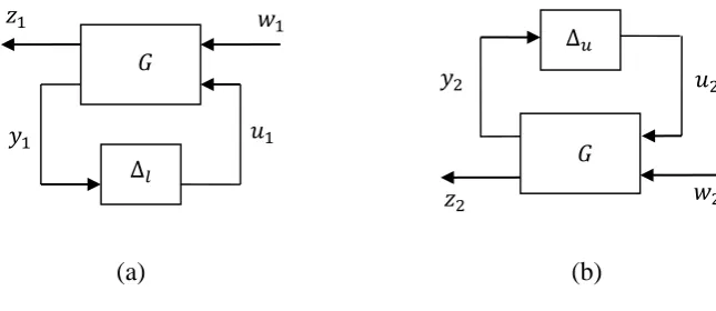
Given a complex matrix Gblock partitioned as:

𝐺 = [𝐺11 𝐺12 𝐺21 𝐺22] ∈ ℂ

31

and two other complex matrices Δ𝑙∈ ℂn2×𝑚2 and Δ𝑢 ∈ ℂn1×𝑚1, we can formally

establish two mappings, namely lower and upper LFT. The lower LFT with respect to Δ_𝑙

is defined as the map:

ℱ_𝑙(𝐺,•) ∶ ℂn2×𝑚2 _{→ ℂ}m1×𝑛1

where

ℱ_𝑙(𝐺, Δ_𝑙) = 𝐺₁₁+ 𝐺₁₂Δ_𝑙( 𝐼 − 𝐺₂₂Δ_𝑙 )−1𝐺₂₁ (2.2.1)

In a similar fashion, an upper LFT with respect to ∆𝑢 is defined as:

ℱ𝑢(𝐺,•) ∶ ℂn1×𝑚1 → ℂm2×𝑛2

where

ℱ_𝑢(𝐺, Δ𝑢) = 𝐺22+ 𝐺21Δ𝑢( 𝐼 − 𝐺11Δ𝑢 )−1𝐺12 (2.2.2)

Obviously, these two mappings are well-defined provided that the inverses exist.

The following representations of ℱ_𝑙(𝐺, Δ_𝑙) and ℱ_𝑢(𝐺, Δ_𝑢) clearly justifies the terminologies of lower and upper LFTs.

(a) (b)

Figure 2.2.1 (a) The lower and (b) the upper LFT 𝐺

∆𝑙

𝑤1

𝑧1

𝑦1 𝑢1

𝐺

𝑤2

𝑧2

𝑢2

∆𝑢

32

By taking 𝐺 as a proper transfer matrix, the lower and upper LFTs defined above are simply the closed-loop transfer matrices from 𝑤₁ to 𝑧₁ and from 𝑤₂ to 𝑧₂ respectively, i.e. [2]:

ℱ_𝑙(𝐺, Δ𝑙) = 𝑇𝑧1𝑤1 and ℱ𝑢(𝐺, Δ𝑢) = 𝑇𝑧2𝑤2 (2.2.3)

Every synthesis problem can be cast as a lower LFT when 𝐺 is interpreted as a generalized plant and Δ𝑙 as a controller to be designed. On the other hand, every analysis problem can

be formulated as an upper LFT when 𝐺 is an interconnection matrix with some structured

Δ_𝑢 representing parametric or unstructured uncertainty [2].

The present work which involves the design problem of deadbeat controller under various constraints is developed based on the lower LFT configuration.

2.3 The general framework:

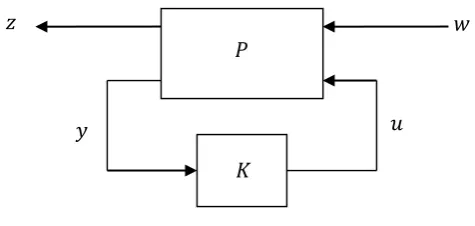
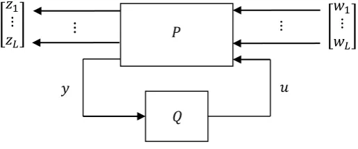
In view of the arguments presented in the previous section, any control problem can be reconfigured as an LFT model. With this motivation, we consider the configuration in figure 2.3.1 as the fundamental framework in this thesis.

Figure 2.3.1 The general framework

In the illustrated block diagram, 𝑃 is the generalised plant which admits the following state space description:

𝑧 𝑤

𝑦 𝑢

𝑃

33

𝑥̇ = 𝐴𝑥 + 𝐵₁𝑤 + 𝐵₂𝑢

𝑧 = 𝐶₁𝑥 + 𝐷₁₁𝑤 + 𝐷₁₂𝑢 (2.3.1)

𝑦 = 𝐶₂𝑥 + 𝐷₂₁𝑤 + 𝐷₂₂𝑢

Intuitively, the generalised-plant transfer function is partitioned as:

𝑃 =           21 21 2 12 11 1 2 1 D D C D D C B B A

= [𝑃11 𝑃12

𝑃₂₁ 𝑃₂₂] (2.3.2)

The controller 𝐾 is described by the state space realization:

𝑥̇_𝐾 = 𝐴_𝐾𝑥_𝐾 + 𝐵_𝐾𝑢_𝐾 (2.3.3)

𝑦_𝐾 = 𝐶_𝐾𝑥_𝐾+ 𝐷_𝐾𝑢_𝐾

We make the standard assumption that the realisations of the plant and the controller are both stabilizable and detectable.

With regards to the (vector) signals, the input signal 𝑤, referred to as the exogenous input, captures the effect of the environment on the plant. It contains disturbance and actuator’s/sensors’ noise-signals. 𝑤 may also contain fictitious inputs injected at any point in the plant. The input signal 𝑢 denotes the inputs manipulated by the controller. The output vector signal 𝑦, known as the measured or sensor outputs, represents the signals accessible to the controller. The regulated variable, denoted by 𝑧, as the name suggests, include all the outputs we wish to regulate or control. Basically, it represents every signal about which we express a specification or constraint. As such, it may include internal states or variables, or even components of 𝑢 and 𝑦. [3, 4, 5]

In order to get the closed-loop transfer function, the output feedback control law:

34

is applied and the equalities 𝑢𝐾 = 𝑦 and 𝑦𝐾 = 𝑢 are imposed. Solving the set of equations

in (2.3.1) for 𝑧 in terms of 𝑤, yields the corresponding input-output characterization of the closed-loop interconnection as:

𝑧 = (𝑃₁₁+ 𝑃₁₂𝐾(𝐼 − 𝑃₂₂𝐾)−1_𝑃

21)𝑤: = 𝐻𝑧𝑤𝑤 (2.3.5)

𝐻_𝑧𝑤, the closed-loop map from the exogenous inputs 𝑤 to the regulated variables 𝑧, contains every closed-loop transfer function of interest. Having compared the above description with (2.2.1), it can be easily inferred that the closed-loop map is in the form of a lower LFT.

Derivation of 𝐻𝑧𝑤 necessitates (𝐼 − 𝑃22𝐾) to be invertible and proper. This, which is

known as the “posedness” condition ensures that all closed-loop maps are well-defined and proper. In other words, this condition ensures that the feedback system makes sense or is physically realizable. The invertibility of (𝐼 − 𝑃₂₂𝐾) is a necessary and sufficient condition for well-posedness, and is equivalent to the invertibility of (𝐼 − 𝑃22(∞)𝐾(∞)) [1, 5]. In most practical systems the feed-through matrix 𝐷22 is zero which

automatically guarantees the existence of the inverse [6]. Therefore for systems with zero feed-through matrix or simply strictly proper systems, the well-posedness is guaranteed.

2.4 Internal stability of the LFT:

35

Internal stability refers to the autonomous system dynamics in the absence of external inputs and so it coincides with the standard notion of asymptotic stability of dynamical systems. Internal stability is a basic requirement for every practical feedback system. This is because all interconnected systems may be unavoidably subject to some nonzero initial conditions and some (possibly small) errors, which in practice cannot be tolerated. Such errors at some points of the closed-loop system may lead to unbounded signals at other points in the interconnection. Through internal stability of the closed-loop system it is ensured that all signals in a system are bounded provided that the injected signals at any locations are bounded.

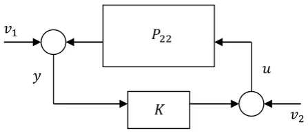
To analyse the internal stability of the LFT configuration of Figure 2.3.1 in terms of the state space description, consider the following corresponding setup for internal stability:

Figure 2.4.1 Setup for internal stability definition

Definition 2.4.1 [8] The LFT interconnection is internally stable if the nine mappings from w, v₁ , and v₂ to z, y, and u are all stable.

In order to limit the number of tedious calculations when deriving the state space realization of the closed-loop transfer matrix, a further assumption is to omit the direct feed-through term 𝐷₂₂. As discussed in the preceding section, this will also ensure the well-posedness of the system. We may restore 𝐷22 ≠ 0 by a loop shifting argument that

absorbs 𝐷₂₂ into 𝐾, in the case that 𝐷₂₂ ≠ 0. The procedure to do this is fully discussed in [6] and is known as loop shifting.

Having imposed the assumption, the closed-loop system dynamical equations reduce to: 𝑤

𝑧

𝑢 𝑃

𝐾 𝑦

𝑣2

36

[_𝑥̇𝑥̇ 𝐾] = [

𝐴 + 𝐵₂𝐷_𝐾𝐶₂ 𝐵₂𝐶_𝐾 𝐵_𝐾𝐶₂ 𝐴_𝐾 ] [

𝑥 𝑥_𝐾] + [

𝐵₁+ 𝐵₂𝐷_𝐾𝐷₂₁ 𝐵₂𝐷_𝐾 𝐵₂ 𝐵_𝐾𝐷₂₁ 𝐵_𝐾 0] [

𝑤 𝑣₁ 𝑣₂]

[ 𝑧 𝑦 𝑢 ] = [

𝐶₁+ 𝐷₁₂𝐷_𝐾𝐶₂ 𝐷₁₂𝐶_𝐾

𝐶₂ 0

𝐷_𝐾𝐶₂ 𝐶_𝐾 ] [_𝑥𝑥

𝐾] + [

𝐷₁₁+ 𝐷₁₂𝐷_𝐾𝐷₂₁ 𝐷₁₂𝐷_𝐾 𝐷₁₂

𝐷₂₁ 𝐼 0

𝐷_𝐾𝐷₂₁ 𝐷_𝐾 𝐼 ] [ 𝑤 𝑣1 𝑣2 ] (2.4.1)

Lemma 2.4.2 [6] The LFT ℱ_𝑙(𝑃, 𝐾) is internally stable if and only if the system matrix

[𝐴 + 𝐵_𝐵 2𝐷𝐾𝐶2 𝐵2𝐶𝐾

𝐾𝐶2 𝐴𝐾 ] is asymptotically stable (Hurwitz).

It should be noted that not every linear fractional transformation is stabilizable. The simplest example which illustrates this is when 𝑃11 is unstable and 𝑃21 = 0.

Lemma 2.4.3 [5] 𝑃 is stabilizable if and only if (𝐴, 𝐵₂, 𝐶₂) is stabilizable and detectable. Thus, from the assumed stabilizability and detactability of 𝑃, the stabilizability and detectability of 𝑃22 is assured.

The ensuing lemma states that 𝑃 and 𝑃₂₂ have identical internal stabilizability properties. This, in turn, leads to the simplification of Figure 2.4.1 to the equivalent configuration of Figure 2.4.2.

Figure 2.4.2 Equivalent diagram to analyse internal stability 𝑃22

𝐾 _𝑣

2

𝑣1

37

Lemma 2.4.4 [6] 𝐾 is an internally stabilizing controller for 𝑃 if and only if it internally stabilizes 𝑃₂₂.

A proper controller 𝐾 which internally stabilizes the plant 𝑃 is said to be admissible. Moreover, such a plant for which there exists at least one stabilizing controller is called a generalized plant. [9]

2.5 Coprime factorization and internal stability:

In the previous section the internal stability of the LFT configuration was discussed through the system state space description. In this and the successive section however, stability is analysed in a different framework, involving the coprime factorization of the constituent systems of the feedback interconnection over the set of proper and stable transfer matrices. Studying the stability problem in this framework is a special case of a more general approach in which the analysis and synthesis problems are formulated based on the fractional representation of the systems, principally developed in [11, 12, 13, 20]. This approach, which has its roots in abstract algebra, considers in the SISO case the transfer functions with the prescribed properties as a ring 𝐻, and then models a given system as the ratio of two transfer functions in 𝐻. This casts the synthesis problem as designing a feedback system which lies in a desired ring of operators when both the plant and compensator are modelled as a quotient of operators from that ring [11]. What makes the procedure highly interesting is that the synthesis problem yields a complete characterization of all compensators which place the feedback system in the ring 𝐻. This approach could be readily extended to the MIMO systems when the transfer matrix has all its entries in 𝐻. The operations of matrix addition and multiplication induced on the set of matrices over 𝐻 by the associated addition and multiplication operations with 𝐻, correspond to parallel and cascade interconnection of such systems [15, 17].

38

the notion of coprime factorization and its characteristics relevant to internal stability theory, which forms the foundation for developing a parameterization of stabilizing controllers in the next section.

Let 𝑅 be a ring and 𝑅𝑛×𝑚 be the set of 𝑛 × 𝑚 matrices whose elements all belong to 𝑅. Every element 𝘧 of 𝐹𝑛×𝑚_{, the set of 𝑛 × 𝑚 transfer matrices, can be factored as an}

element of the field of fractions associated with the ring 𝑅 and expressed as the ratio of two matrices 𝑁 and 𝐷, as 𝘧 = 𝑁𝐷−1 where 𝑁, 𝐷 ∈ 𝑅𝑛×𝑚 and det 𝐷 ≠ 0. The pair (𝑁, 𝐷)

is referred to as a right fractional representation of 𝘧. In a similar way, the left fractional representation of every 𝘧 ∈ 𝐹𝑛×𝑚 _{is defined as 𝘧 = 𝐷̃}−1_{𝑁̃ where again 𝑁̃, 𝐷̃ ∈ 𝑅}𝑛×𝑚 _and det 𝐷̃ ≠ 0 [11, 13, 20, 165, 166].

Definition 2.5.1 [13] Two matrices 𝑁, 𝐷 ∈ 𝑅𝑛×𝑚 are called right coprime if there exists matrices 𝑋, 𝑌 ∈ 𝑅𝑛×𝑚 _{such that:}

𝑋𝐷 − 𝑌𝑁 = 𝐼_𝑚 (2.5.1)

which can be stated equivalently as:

Definition 2.5.2 [19] Two matrices 𝑁, 𝐷 ∈ 𝑅𝑛×𝑚 are right coprime if they have equal number of columns and there exists matrices 𝑋, 𝑌 ∈ 𝑅𝑛×𝑚 _{such that:}

[𝑋 𝑌] [ 𝐷

−𝑁] = 𝐼𝑚 (2.5.2)

This is equivalent to the matrix [𝐷𝑇 _{− 𝑁}𝑇_]𝑇 _{being left-invertible in 𝑅}𝑛×𝑚_.

39

Definition 2.5.3 [13] In definition 2.5.2, if 𝐷 is non-singular, 𝘧 = 𝑁𝐷−1 is referred to right coprime factorization (r.c.f) of 𝘧.

The notions of left coprime and left coprime factorization can be defined analogously.

Definition 2.5.4 [19] For 𝘧 ∈ 𝐹𝑛×𝑚 _{, 𝑁̃, 𝐷̃ ∈ 𝑅}𝑛×𝑚 _{with equal number of rows, and 𝐷̃}

non-singular, 𝘧 = 𝐷̃−1𝑁̃ is called the left coprime factorization (l.c.f) of 𝘧 if there exists matrices 𝑋̃, 𝑌̃ ∈ 𝑅𝑛×𝑚 _{such that:}

[𝐷̃ 𝑁̃] [ 𝑋̃

−𝑌̃] = 𝐼𝑛 (2.5.3)

This is equivalent to the matrix [𝐷̃ 𝑁̃] being right-invertible in 𝑅𝑛×𝑚. The Bezout identity corresponding to (2.5.3):

𝐷̃𝑋̃ − 𝑁̃𝑌̃ = 𝐼𝑛 (2.5.4)

is referred to left Bezout identity or left Diophantine identity.

The ring concerning the internal stability problem being considered here, is the set of proper and stable rational transfer matrices, namely the ring ℝ𝐻∞ [19, 165, 166]. The

setting in which 𝑅 = ℝ𝐻_∞, not only catches the usual notion of instability as the result of existing unstable closed-loop poles, but also excludes the possibility of unstable pole-zero cancellations between the plant and controller. These will become clear as we proceed. From coprime fractional representation over ℝ𝐻_∞, some significant properties imposed by coprimeness can be inferred, which reveals the benefits of studying stabilization problem in a ring theoretic setting.

In view of Lemma 2.4.4 which establishes the equivalence between the stabilization of the plant 𝑃 and that of 𝑃₂₂ (figure 2.3.1), all the subsequent discussion is made about 𝑃₂₂. Suppose that 𝑃22 has a r.c.f over ℝ𝐻∞ as 𝑃22 = 𝑁𝑟𝐷𝑟−1, where 𝑁𝑟, 𝐷𝑟 ∈ ℝ𝐻∞. Rewriting

40

Remark 2.5.5 [15] Instabilities of 𝑃22 are completely characterized by the denominator

of a r.c.f of 𝑃₂₂, i.e. the unstable poles of 𝑃₂₂ are precisely the unstable zeros of 𝐷_𝑟.

Theorem 2.5.6 [20] The pairs 𝑁₁, 𝐷₁ ∈ ℝ𝐻_∞ and 𝑁₂, 𝐷₂ ∈ ℝ𝐻_∞ define right coprime factorizations of 𝑃₂₂ as 𝑃₂₂ = 𝑁₁𝐷₁−1 = 𝑁₂𝐷₂−1, if and only if:

[𝐷1 𝑁1] = [

𝐷₂ 𝑁2] 𝑊

where 𝑊, 𝑊−1 _{∈ ℝ𝐻}

∞. In other words, 𝑊 is ℝ𝐻∞-unimodular.

Definition 2.5.7 [46]Let ℛ be a ring and ℛ𝑙×𝑚 denote the 𝑙 × 𝑚 matrices with elements from ℛ. A matrix 𝑈 ∈ ℛ𝑚×𝑚 _{is unimodular, if and only if det 𝑈 is a unit in ℛ, i.e. it is a}

matrix in ℛ𝑚×𝑚 whose inverse belongs to ℛ𝑚×𝑚 too. Such matrices are termed

ℛ-unimodular and designated as 𝑈[ℛ].

Theorem 2.5.6 may be stated in the equivalent form of the following remark.

Remark 2.5.8 [22] A right coprime factorization is unique up to a unimodular common right divisor.

This remark, in turn, leads to the following important observation:

Remark 2.5.9 [17] Cancellation of instabilities, between the numerator and denominator of a r.c.f is not allowed. In this sense, a r.c.f is irreducible.

This makes clear the notion of irreducible quotient of stable elements mentioned earlier. A similar theorem and remarks hold analogously for a l.c.f of 𝑃22= 𝐷𝑙−1𝑁𝑙.

41

The following theorem establishes the connection between the right and left coprime factorizations.

Theorem 2.5.10 [23] Assume that 𝑃22 admits both right and left coprime factorization as 𝑃₂₂ = 𝑁_𝑟𝐷_𝑟−1_{= 𝐷}

𝑙−1𝑁𝑙, with 𝑁𝑟, 𝐷𝑟, 𝑁𝑙, 𝐷𝑙∈ ℝ𝐻∞, for which there exists 𝑋𝑟, 𝑌𝑟 ∈ ℝ𝐻∞

such that 𝑋_𝑟𝐷_𝑟− 𝑌_𝑟𝑁_𝑟 = 𝐼. Then, there exist 𝑋_𝑙, 𝑌_𝑙∈ ℝ𝐻_∞ such that:

[ 𝑋𝑟 −𝑌𝑟 −𝑁𝑙 𝐷𝑙 ] [

𝐷_𝑟 𝑌_𝑙 𝑁𝑟 𝑋𝑙] = [

𝐼 0

0 𝐼] (2.5.5)

This is referred to as the doubly coprime factorization or generalized Bezout identity, and is the cornerstone in the parameterization of all stabilizing controllers, as will be shown in the next section.

The notion of coprimeness readily extends to continuous-time as well as discrete-time systems, lumped and distributed systems, and one- and multi-dimensional systems. Therefore, all these situations can be captured within the single framework of stable factorization approach [15, 13].

2.6 Parameterization of all stabilizing controllers:

In the preceding section, the notion of coprime factorization over ℝ𝐻_∞ was defined. The main intention was to express a system as an irreducible quotient of two rational proper and stable elements in ℝ𝐻∞. In the current section, the relation between coprime

factorization over ℝ𝐻_∞ and internal stability of the LFT feedback interconnection of figure 2.3.1 will be discussed. Moreover, parametric characterization of all compensators which stabilize a given plant will be developed. As stated in Lemma 2.4.4, internal stability of 𝑃 in the basic configuration of figure 2.4.1 is equivalent to that of 𝑃₂₂. This accordingly suggested considering 𝑃22 as the system to be stabilized in the associated

configuration of figure 2.4.2. To motivate what follows, take the case where 𝑃₂₂ is a scalar function with coprime factorization 𝑃₂₂ = 𝑛𝑑−1_{, and let 𝑥, 𝑦 ∈ ℝ𝐻}

∞ being scalar

42

a stabilizing controller for 𝑃22. To see this, note that in figure 2.4.2 the mapping from [𝑣₁𝑇 _𝑣

2𝑇]𝑇 to [𝑢𝑇 𝑦𝑇]𝑇 is:

1 1 − 𝐾𝑃₂₂[

1 𝐾

𝑃22 𝐾𝑃22] = 1 𝑥𝑑 − 𝑦𝑛[

𝑥𝑑 𝑦𝑑 𝑥𝑛 𝑦𝑛] = [

𝑥𝑑 𝑦𝑑 𝑥𝑛 𝑦𝑛]

Since all 𝑛, 𝑑, 𝑥, and 𝑦 elements are in ℝ𝐻_∞, it is easily inferred that the closed-loop system is internally stable.

Noticing that for any 𝑞 ∈ ℝ𝐻_∞ the following Diophantine equation is satisfied:

(𝑥 − 𝑛𝑞)𝑑 − (𝑦 − 𝑑𝑞)𝑛 = 1

it follows analogously that:

𝐾 =𝑦 − 𝑑𝑞 𝑥 − 𝑛𝑞

is an admissible controller for any 𝑞 ∈ ℝ𝐻∞. Hence, coprime factorization of 𝑃22

generates a family of stabilizing controllers over the proper and stable (but otherwise arbitrary) parameter 𝑞. The idea can be extended to the general matrix case in the form of following theorem.

Theorem 2.6.1 [6, 13] Suppose 𝑃 is stabilizable. Let 𝑃₂₂ = 𝑁_𝑟𝐷_𝑟−1= 𝐷_𝑙−1𝑁_𝑙 be right and left coprime factorizations of 𝑃22, and let its corresponding doubly coprime

factorization as:

[ 𝑋𝑟 −𝑌𝑟 −𝑁𝑙 𝐷𝑙 ] [

𝐷_𝑟 𝑌_𝑙 𝑁𝑟 𝑋𝑙] = [

𝐼 0

0 𝐼] (2.6.1)

Then the following statements are equivalent:

43

2. 𝐾 = 𝑈𝑟𝑉𝑟, where

[𝑈_𝑉𝑟 𝑟] = [

𝐷_𝑟 𝑌_𝑙 𝑁_𝑟 𝑋_𝑙] [

−𝑄

𝐼 ], 𝑄 ∈ ℝ𝐻∞ (2.6.2)

3. 𝐾 = 𝑉_𝑙−1𝑈𝑙, where

[𝑉𝑙 −𝑈𝑙] = [𝐼 𝑄] [_−𝑁𝑋𝑟 −𝑌𝑟

𝑙 𝐷𝑙 ], 𝑄 ∈ ℝ𝐻∞ (2.6.3)

4. 𝐾 = ℱ𝑙(𝐾𝑠, 𝑄) (2.6.4)

in which

𝐾_𝑠 = [𝑋𝑟 −1_𝑌

𝑟 −𝑋𝑟−1 𝑋_𝑙−1 𝑋_𝑙−1𝑁_𝑟] = [

𝑈𝑟𝑉𝑟−1 −𝑉𝑙−1

𝑉_𝑟−1 𝑉_𝑟−1𝑁_𝑟] (2.6.5)

The theorem clearly exhibits the relationship between coprime factorization and stabilizing compensators. In other words, coprime factorization and stabilization are intimately connected. The doubly coprime factorization, defined by generalized Bezout equations, leads to a parametric characterization of all controllers which internally stabilizes a given plant. All stabilizing controllers are expressed as a coprime factorization, including the elements of a doubly coprime factorization of the system to be stabilized and a proper stable but arbitrary parameter. In fact, the doubly coprime factorization is equivalent to the choice of a single stabilizing controller, and the theorem renders the whole set of stabilizing controllers constructed from that single choice, termed

𝐾_𝑠. This is sometimes known as the nominal or central controller and the set of stabilizing controllers is obtained through augmenting 𝐾_𝑠.

As mentioned in the last part of theorem 2.6.1, stabilizing compensators have the structure of a linear fractional transformation. In regards to the LFT construction of the closed-loop map 𝐻_𝑧𝑤 in (2.3.5) and the composition of two LFTs formulated in [6] and designated by

44

𝐻𝑧𝑤 = ℱ𝑙(𝑃, 𝐾) = ℱ𝑙(𝑃, ℱ𝑙(𝐾𝑠, 𝑄)) = ℱ𝑙(𝐶𝑙(𝑃, 𝐾𝑠), 𝑄) (2.6.6)

Denoting the composition 𝐶𝑙(𝑃, 𝐾𝑠) by 𝑇, gives the closed-loop map as:

𝐻_𝑧𝑤 = ℱ_𝑙(𝑇, 𝑄) (2.6.7)

Accordingly, the closed-loop map description is given by:

𝐻𝑧𝑤 = ℱ𝑙( [

𝑃₁₁ 𝑃₁₂

𝑃₂₁ 𝑃₂₂] , 𝐾) = ℱ𝑙( [

𝑇₁₁ 𝑇₁₂

𝑇₂₁ 0 ] , 𝑄) = 𝑇11+ 𝑇12𝑄𝑇21 (2.6.8)

which is clearly an affine parameterization in the design parameter 𝑄. This is known as the 𝑄-parameterization or Youla-Jabr-Bongiorno-Kucera (YJBK) parameterization, which was first developed in [25]. Thus, the given parameterization of all stabilizing compensators replaces the linear fractional parameterization ℱ_𝑙(𝑃, 𝐾) of the closed-loop maps of interest with the affine parameterization 𝑇11+ 𝑇12𝑄𝑇21. In many synthesis

problems, these closed-loop maps form the design objectives of optimization problems with stability as a constraint. The 𝑄-parameterization reduces the problem of search or optimization over the set of stabilizing controllers to a search or unconstrained optimization over the parameter 𝑄 ∈ ℝ𝐻_∞.

By substituting the parameterized set of stabilizing controllers of (2.6.2) and (2.6.3) in (2.6.1), the equality (2.6.1) can be expressed as:

[ 𝑉𝑙 −𝑈𝑙 −𝑁_𝑙 𝐷_𝑙 ] [

𝐷𝑟 𝑈𝑟 𝑁_𝑟 𝑉_𝑟] = [

𝐼 0

0 𝐼] (2.6.9)

It is evident that, by construction, 𝑈_𝑟 , 𝑉_𝑟, 𝑈_𝑙, 𝑉_𝑙∈ ℝ𝐻_∞, i.e. all are proper and stable. From the Bezout equations ensuing from (2.6.9) as:

𝑉_𝑙𝐷_𝑟− 𝑈_𝑙𝑁_𝑟 = 𝐼 (2.6.10)

𝐷_𝑙𝑉_𝑟− 𝑁_𝑙𝑈_𝑟 = 𝐼